Abstract
The fast and reliable processing of medical images is of paramount importance to adequately generate data to feed machine learning algorithms that can prevent and diagnose health issues. Here, different compressed sensing techniques applied to magnetic resonance imaging are benchmarked as a means to reduce the acquisition time spent in the collection of data and signals that form the image. It is shown that by using these techniques, it is possible to reduce the number of signals needed and, therefore, substantially decrease the time to acquire the measurements. To this end, different algorithms are considered and compared: the iterative re-weighted least squares, the iterative soft thresholding algorithm, the iterative hard thresholding algorithm, the primal dual algorithm and the log barrier algorithm. Such algorithms have been implemented in different analysis programs that have been used to perform the reconstruction of the images, and it was found that the iterative soft thresholding algorithm gives the optimal results. It is found that the images obtained with this algorithm have lower quality than the original ones, but in any case, the quality should be good enough to distinguish each body structure and detect any health problems under an expert evaluation and/or statistical analysis.
Keywords:
compressed sensing; medical resonance imaging; IRLS; ISTA; IHTA; primal dual algorithm; log barrier algorithm MSC:
94A20; 94A12; 94A40
1. Introduction
As the years go by and scientific knowledge increases and refines, theories are updated and improved, giving rise to more reliable and efficient technological applications. For example, within the field of signal processing, in the past, a camera with n pixels needed n signals to form the image. In 1949, however, with the Shannon–Nyquist theorem [1], it was shown that it was possible to form the same image with fewer signals. This theorem establishes that it is feasible to recover a signal if it is sampled uniformly at a rate of at least twice its Fourier bandwidth, that is, it allows a continuous signal to be reconstructed with a discrete sequence of acquired samples. However, for some applications, such as radar imaging or different imaging modalities outside of visible wavelengths, the required sampling rate may be so high that it is impossible for state-of-the-art samplers to achieve such values. Furthermore, due to the large number of samples collected, it is necessary to compress them [2]. In 2006, Donoho and the team consisting of Romberg, Candès and Tao introduced the concept known as compressed sensing (CS) [3,4], which substantially simplified the acquisition process.
CS is an alternative technique to the Shannon–Nyquist sampling theorem. With this approach, it is possible to reconstruct a signal from a few random measurements using some non-linear techniques, as long as the original signal is compressible or sparse. A sparse signal has most of its coefficients as zero, and only a few contain all the information. It is possible to obtain this type of signal through a basis transformation. For example, a sinusoidal signal of a given frequency obtained with a voltmeter as a function of time is not sparse. However, if the Fourier transform is applied, the signal has an associated peak at that frequency. The rest of the values are zero. Therefore, in the Fourier domain, [5] is sparse. Moreover, there are different wavelet transformations that allow this sparsity, such as Daubechies [6] or the Tight-Frame [7].
The main objective of CS is to reduce the number of coefficients necessary to obtain the desired resolution and quality for the representation of the object of interest. To achieve this, it uses a mathematical function called a norm. The norm of a vector x (vector notation is shown in bold) of length n is expressed as follows:
In the case , the norm consists of the number of non-zero elements in the vector x. The norm () gives as a result the sum of the elements of the vector. The norm is widely used to compute the Euclidean distance [8].
The CS problem can be described as the reconstruction of the vector x of dimension n, from the measurements , of dimension m, and the random measurement matrix A, known as the sensing or measurement matrix, of dimensions m × n.
The solution to this problem depends on its typology as follows:
- If m > n and rank(A) = n (purely overdetermined linear system), the linear system is solved via least squares:The reconstruction error of y: is non-null.
- In the purely underdetermined case (m < n and rank(A) = m), there is an infinite set of solutions that belong to a linear variety oriented by the null space of A. This is the typical case of under-sampling, that is, the number of samples in A (length of y ) is less than the original size of x. In this case, the minimum norm solution is written as follows:since it does not have components in the null space of A. This solution is sparse in the system of reference ().
The sparse problem treated in this paper consists in finding the sparser solution in the norm, which is the same to impose sparsity in the canonic basis set of :
Minimization in norm requires an exhaustive search over all possible sparse combinations. Since it requires a large computational cost, this minimization is replaced by the convex minimization problem in . This problem is determined as
and it is known as basis pursuit (BP). In more complex situations, the measurements obtained are corrupted by an unknown noise, which is denoted as e. Therefore, . The reconstruction problem is written as follows:
where . This problem is known as BP denoising (BPDN) [9].
This is equivalent to imposing that the linear system is incompatible due to measurement noise. BPDN is a constrained problem, whose solution can be approached by the following unconstrained optimization problem:
The parameters and are related but, generally, the relationship between them is not analytical and cannot be estimated [10].
The CS technique has various applications in many fields, e.g., underwater imaging [11], wireless monitoring of structural health [12] and 3D visualization of the oxidation state of iron in FeO/FeO [13]. In this document, CS is used in medical imaging, in particular, with images obtained by nuclear magnetic resonance (NMR).
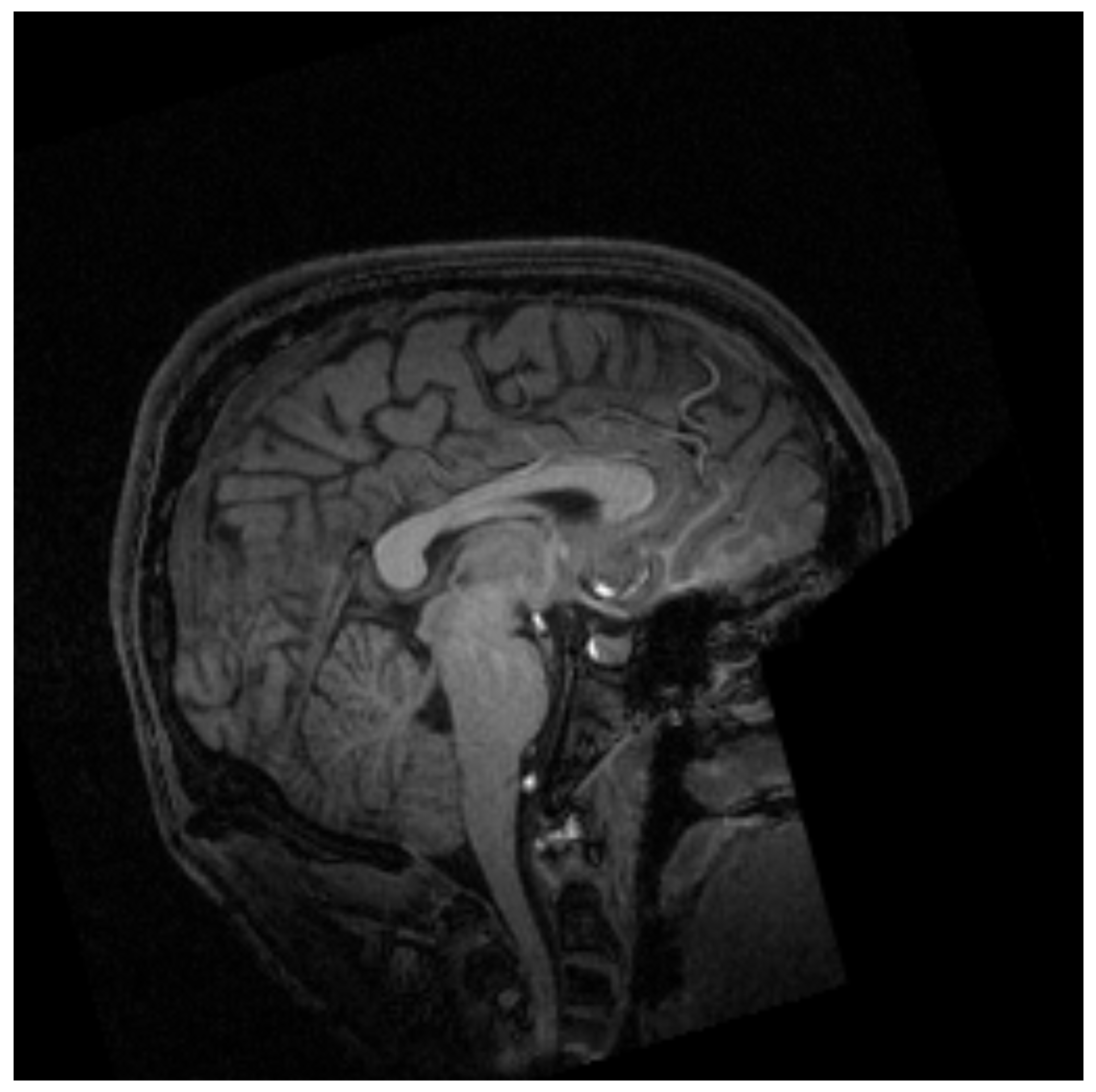
MRI is a non-invasive technique widely used in medicine to obtain the necessary medical images for further diagnosis. This technique is based on the physical phenomenon of resonance. It consists of the transition between different energy states when an atomic nucleus is introduced into an external magnetic field of a characteristic frequency. This frequency, known as the Larmor frequency, corresponds to the precession frequency of the protons inside the nucleus. When a magnetic field is applied, the protons absorb the energy and raise it to a higher level. Once the magnetic field is removed, the protons decay to the ground state. MRI measures the time and energy released from this last transition. Due to its environment, those two values will be different for each proton. Then, applying the inverse Fourier transform to the obtained data, the image is created with different contrast for each component of the body [14] as shown in Figure 1.

Figure 1.
Example of magnetic resonance imaging of the cranial region [15].
This technique makes it possible to distinguish different components of the human body, particularly soft tissues, such as muscles, tendons, ligaments, fat, etc. Not only that but it also makes it possible to differentiate between bones and organs [14]. The images can be in any direction or part and can even be made of animals, for example, a mouse [16]. In addition, magnetic resonance can be used as a spectroscopy technique in biochemistry: it allows knowing the three-dimensional and dynamic structure of biological molecules [17]. In addition, its main advantage over other techniques, such as computed tomography or X-rays, is the lack of ionizing radiation, which makes MRI exams safe for the patient. For these reasons, its multiple uses, and its high-resolution images, MRI is known as the crown jewel in medical imaging [18].
Despite the many advantages mentioned above, MRI has some drawbacks: patients with pacemakers or metal prostheses can be injured by the strong magnetic field (up to 3T), so they cannot be examined. In addition, due to the reduced space and high noise level of the machine, it can generate stress or anxiety. In addition to these disadvantages, there are many more safety precautions that must be taken into account when taking an exam. In addition, the maintenance of the machine components and the tests are very expensive. Finally, it takes a long time to acquire the data needed to build the image, approx. 40 min [19].
In this article, we present a methodology to reduce the MRI acquisition time by using three different CS algorithms. Different MRI images of the head are considered and reconstructed with fewer measurements, leading to a reduction in the acquisition time. In the algorithms, a smaller number of data is introduced than the real image, the time that the algorithm takes in the reconstruction is measured, and the error is made. This study then paves the way for shorter MRI exams.
General Contributions
The general contributions of this study are the following:
- Different compressed sensing algorithms used to reconstruct various medical images are evaluated and compared.
- The acquisition time and the number of measurements performed are reduced and minimized.
- The error in the reconstructed image is minimized by adjusting the regularization and optimization parameters in the algorithms.
The article is organized as follows: first is an overview of previous works in Section 2; in Section 3, the CS algorithms employed to reconstruct the image are described, and it is shown how they can be applied in MRI. In Section 4, the results are presented and discussed (reconstructed images, acquisition time and error). The article finishes with the conclusions.
2. Related Works
Compressed detection techniques have been applied to the reconstruction of magnetic resonance images. One of the first papers in this field was presented by Donoho in 2006, in which he presented the concept of compressed sensing and demonstrated its potential application to magnetic resonance imaging reconstruction. Compressed detection is based on the assumption that most medical images are underrepresented in some domain, allowing accurate reconstruction from a limited set of [3,20] measurements. This breakthrough opened up new possibilities for speeding up MRIs, making them more feasible and comfortable for patients while reducing motion artifacts.
Following Donoho’s groundbreaking work, numerous algorithms have been proposed to improve and optimize the compressed detection reconstruction process for MRI in order to achieve better image quality. They have been extensively evaluated through simulations and experiments. The main goal of these experiments is to assess the quality and accuracy of the reconstructed images, as well as determining the robustness of the algorithm under various conditions.
Among these algorithms, the iterative re-weighted least squares (IRLS) was proposed as an improvement of the traditional compressed detection algorithm, improving the convergence and the quality of image reconstruction [20]. This algorithm led to a successful reduction in the acquisition time while preserving image quality, enabling fast and efficient MRI scans [21]. Daubechies et al. (2004) introduced the iterative smooth threshold algorithm (ISTA). ISTA is an optimization-based approach that promotes sparseness in the reconstructed image, allowing for more efficient image reconstruction with fewer measurements [22]. In parallel, IHTA was introduced, which broadens the threshold idea to promote scarcity in MRI reconstruction. IHTA aims to recover sparse signals more accurately by iteratively discarding the least-significant coefficients [23]. The primal dual algorithm (PDA) is another approach that has gained attention in the context of compressed detection for MRI reconstruction. PDA takes advantage of a dual variable formulation to promote scarcity and encourage more efficient and accurate retrieval of MRI signals [24]. A new variant of the primal dual algorithm (PDA) was proposed for MRI reconstruction [4] that improves the algorithm’s ability to handle complex MRI structures more effectively, offering better image reconstruction [25]. The LBA takes advantage of the logarithmic barrier function to approximate the non-smooth L1 norm, which promotes sparseness in the signal domain. This algorithm effectively tightens the sparseness constraints and improves the quality of images reconstructed from heavily undersampled data [26].
In addition, there are numerous studies comparing compressed detection algorithms to assess their performance under various conditions [27,28,29]. The use of CS in single pixel detectors has also been simulated to achieve high-resolution images [30,31]. Furthermore, the integration of deep learning techniques with compressed detection has gained attention in recent years. Deep learning-based approaches have shown great potential to improve the reconstruction quality and robustness of compressed detection methods, making them even more attractive for MRI applications [32,33].
This article focuses on the study of these algorithms (IRLS, ISTA, IHTA, PDA, and LBA), more classical algorithms that minimize the l1 norm and the TV norm, and do not require any parallelization or special hardware support, such as GRAPPA [34].
3. Materials and Methods
MRI receives the data of proton relaxation and stores them in the frequency space so that with the inverse Fourier transform, it is possible to construct the image. The CS problem applied to this case can be written as
where y are the frequency samples collected by the machine, F is the Fourier measurement matrix, x is the image to be constructed, and is the noise randomly distributed. An inverse linear problem has to be solved to recover the data that form the image from the measurements; the measurement matrix which associates a frequency to a value in the grey scale is used. Object x can be an image in 2D or 3D, but it is represented as a vector by concatenation.
In the ideal case, in which enough measurements are taken (), Equation (8) can be solved by applying the inverse Fourier transform on the frequencies:
To reduce the acquisition time, fewer measurements are taken. Therefore, Equation (8) has infinite solutions, which can be solved with minimization algorithms. In this article, to reconstruct the image, five possible methods are used: iterative re-weighted least squares (IRLS), iterative soft threshold (ISTA), iterative hard threshold (IHTA), a primal dual algorithm (PD) and a log barrier algorithm (LB). The first three algorithms belong to the category of greedy algorithms. They have less accuracy in the reconstruction but are less expensive and simpler. PD and LB are convex algorithms; the error is minor, but it takes a lot of computational resources [9]. All those algorithms shown below are iterative because of the large storage size of A.
3.1. Iterative Re-Weighted Least Squares
The first algorithm, IRLS, solves the minimization problem without restrictions (Equation (7)). To achieve this, it replaces the minimization with the norm with a given weight represented by the diagonal matrix W in each iteration k. This matrix is updated by
where is the dumping factor, which is reduced at each iteration. In order to obtain the reconstructed signal, the algorithm solves Equation (11), obtained from the unconstrained Lagrangian, until it reaches a certain number of iterations or the solution converges, i.e., , where is the minimum error [10]:
3.2. Iterative Soft Threshold Algorithm
The next algorithm, ISTA, solves the same minimization problem as the previous algorithm (Equation (7)). In this case, the function called the soft threshold is used:
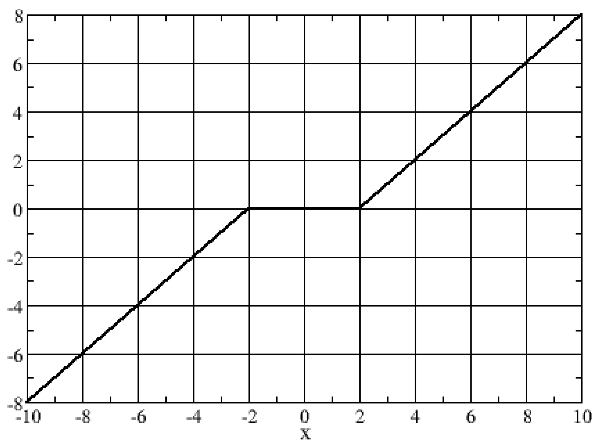
This, shown in Figure 2, tries to decrease the amplitude of the coefficients with noise. For example, if the amplitude of the signal is small, the noise and the number of data which provide information are of equal magnitude. The data contain little information and, therefore, the function returns 0. For larger amplitudes, the noise is very small compared to the intensity of the real signal, and thus the function subtracts the part associated with noise [35].
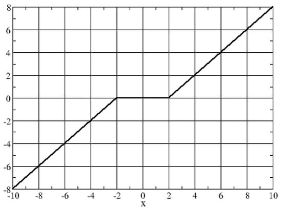
Figure 2.
Soft Threshold rule with .
In order to obtain the reconstructed signal with this algorithm, it is necessary to calculate the Landweber iteration, which is defined as
where a is the largest eigenvalue of the matrix . The solution is calculated with the soft threshold rule, which is written in a more compact way:
In each iteration, the value of should be reduced in order to achieve convergence [10].
Over the years, ISTA have had a lot of improvements in order to reduce the acquisition time or to obtain a better resolution. For example, changing the thresholding function to Equation (15), called the p-thresholding function, the technique penalizes small coefficients and shrinks more values to zero. If , the equation reduces to soft thresholding (Equation (12)) [36]:
Another algorithm which improves the convergence speed, which is the main ISTA problem, is called fast ISTA (FISTA), which relies on the simplicity of the computation of the proximal map of norm. If the gradient algorithm is applied in Equation (6), the following iterative equations are obtained:
where is the step size updated in each iteration. Using this idea with the unconstrained problem (Equation (7)), an iterative scheme is obtained, which can be seen as a proximal regularization of . It is written as
By using FISTA, the number of iterations required to obtain an optimal solution is less than that of ISTA, as it improves the convergence rate [37]. However, there is no simple solution to the non-smooth part . In order to solve this, it is possible to approximate this term by its Moreau envelop, which is smooth [38]. This strategy is also used in projected ISTA (pISTA) and projected FISTA (pFISTA), in which the unconstrained model is converted into a much simpler form, where the objective function can be separated, and the orthogonal projection operator is introduced [39].
It is clear that many ways to optimize MRI and its different sequences have been proposed to improve its stability, memory consumption and reconstruction time [40,41], but ISTA is still a good way for signal reconstruction because it stands out for its simplicity.
3.3. Iterative Hard Threshold Algorithm
As mentioned in Section 1, solving the CS problem in the norm is very expensive. However, IHTA handles this problem if the data have noise, i.e.,
In this algorithm, the following function is defined similarly to ISTA:
In this function, if the signal is of the same magnitude as the noise, it eliminates those values; otherwise, it does not alter the value [10]. In this algorithm, the Landweber iteration is also calculated by Equation (13), and the solution is obtained by
3.4. Primal Dual Algorithm
PD algorithms for linear programming are used to solve Equation (5) among others. The standard form in linear programs is
where each of the is a linear functional for and . This algorithm finds the optimal and the dual vectors , , which satisfies the Karush–Kuhn–Tucker conditions by solving this system of nonlinear equations with Newton’s method [42,43]:
So in the inner loop of the PD algorithm, Newton’s method is applied. Conjugate gradients are used in Equation (22) in order to obtain the step direction . Then, the solution is updated by the next equation:
3.5. Log-Barrier Algorithm
The BPDN problem (Equation (6)) can be modeled as second-order cone programs (SOCPs), i.e., it can be written as a linear program Equation (21), where represents a second-order conic. This method consists of transforming the minimization problem into a series of linear problems in y:
Each one of these subproblems are solved with a high degree of accuracy with Newton’s method to obtain . In each iteration k, is updated so that [43].
3.6. Application of the Algorithms to MRI
Previous algorithms have been used to reduce the MR acquisition time. Since it was not possible to access an MRI machine, the code was designed to read actual MRI images, decompose the data, and store them as vector x. This code also generates the measures matrix A as a function to avoid memory problems due to the large size of the matrix. The measurements that would be obtained in IRM y are evaluated by A and x. The measure matrix function computes the Fourier transform of x and randomly orders its coefficients. The algorithms were applied to y, and the signal and the reconstructed image were obtained. The code also allows to obtain the time it takes to perform the algorithms and the error between the original signal and the reconstructed one. Finally, the regularization and optimization parameters in the algorithms were adjusted so that the error in the reconstructed image was minimal.
The objective of this article is to evaluate and compare different algorithms to reduce the acquisition time so that the number of measurements performed is less than the number necessary to build the original image. In all cases, when the image is read, some values are randomly selected, which are stored in x; then, y is obtained, and the token is reconstructed.
Several images were analyzed with the algorithms to obtain the time and error parameters as a function of the number of measurements. With these results, the best algorithm was selected to carry out the reconstruction applied to MRI and the minimum number of measurements necessary to be able to distinguish all the components of the image.
4. Results and Discussion
Medical imaging acquisition is greatly enhanced by the use of compressed detection techniques since, as discussed above, it is possible to reconstruct a given signal (image) using only a few random measurements. This can substantially increase the speed and accuracy of the acquisition process and lead to better image qualities for certain medical devices, such as those using MRI, which often take a long time to take. This was verified in this section, which presents results after applying the CS algorithms in medical images obtained with magnetic resonance. Several images of the head of the human body obtained from the database of the University of South Carolina [15] were analyzed. Two images commonly used to assess for medical problems were taken: an axial slice of the brain and an axial section of the face and neck region, both at 2048 × 2048 resolutions. The first image is challenging because the brain area does not have much resolution, and it is difficult to distinguish particular features. The second image shows more contrast between different tissue types and is easier to assess.
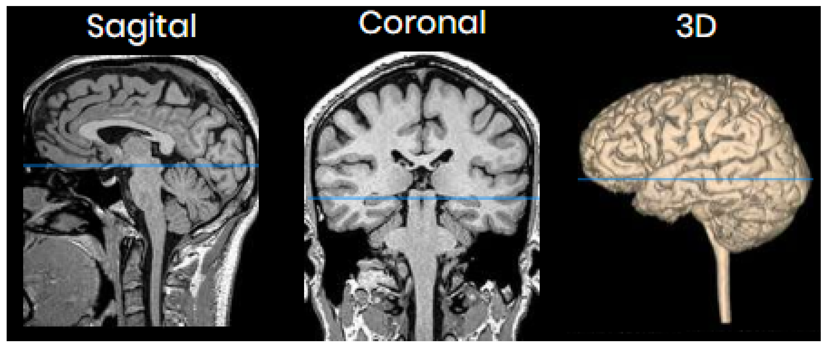
One of the images used in the simulations is shown in Figure 3. The image corresponds to an axial section of the brain in the plane marked by the blue lines in Figure 4. In it, the orbit of the eyes can be distinguished in the lower part. Fat appears with a very strong signal, while water and cerebrospinal fluid have a very low intensity.
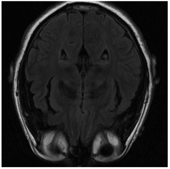
Figure 3.
MRI image of an axial slice of the brain. In the area below are the eye orbits [15].
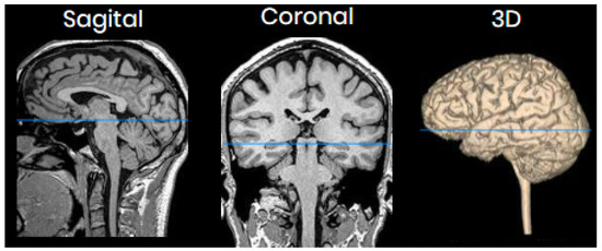
Figure 4.
Images of sagittal, coronal and 3D slices of the brain. The blue line shows the plane corresponding to the image in Figure 3.
The image is blurred in the left orbit, which is an example of an artifact. An artifact is a distortion in the image that has no relation to the subject of the studied body region. In this case, it is generated by the movement of the patient [44]. Artifacts must be recognized, as they can simulate non-existent medical conditions or cover up real problems. In this case, its origin is clear, but in general, it is necessary to know the different types of artifacts that can be produced in order to be able to distinguish and address them properly. The impact of artifacts on the reconstruction process depends on their size. If the artifact is not too large, reconstruction can smooth it out and produce an image without its effect. In this sense, the best algorithm that can deal with artifacts is PD because it leads to clearer and blur-free images as will be seen.
Below are the images and the parameters obtained from the reconstruction, as well as the time and error of each algorithm based on the data taken from the original image.
In the IRLS reconstruction, only the shape of the head and the orbits are detected in the first measurements, while the white matter is not distinguishable (Figure 5 top). When 70% of the data is available (Figure 5 middle), the white matter can be distinguished but with little intensity. When the intensity of the orbits increases, the effect of the artifact begins to be noticed. If the algorithm is run with all available data (Figure 5 bottom), the edge resolution is increased, but white matter signal intensity is lost. That makes their identification more difficult.

Figure 5.
Reconstruction of the image in Figure 3 using IRLS with (top), (middile) and (bottom) of taken measurements.
As in IRLS, the ISTA algorithm first detects the areas of highest intensity in the first measurements without distinguishing the white matter (Figure 6 top). If the number of input data is increased, the border resolution increases, but it is still difficult to differentiate the white matter (Figure 6 middile). Finally, the resolution increases until the shape of the fat is detected (Figure 6 bottom).

Figure 6.
Reconstruction of the image in Figure 3 using ISTA with (top), (middle) and (bottom) of taken measurements.
If IHTA is used for the reconstruction, more noise is detected on the inside of the head (where the white matter should be) with 30% of the initial signal values (Figure 7 top). With 70% of measurements (Figure 7 middle), an image similar to the same case was obtained with ISTA, but the target has more intense signals, which allows to distinguish better. The resolution increases as more data are added. However, when 100% of the data is reached (Figure 7 bottom), the white matter is not detected, it appears black.

Figure 7.
Reconstruction of the image in Figure 3 using IHTA with (top), (middle) and (bottom) of taken measurements.
With the PD algorithm, the object is much clearer with lower measurements. With 30% of the initial values (Figure 8 top), the structure inside the head can be recognized and delimited, even if it is of low intensity. As the number of measurements increases, the images obtain better resolution. At 70% (Figure 8 middle), the image is similar to the original. Finally, at 100% (Figure 8 bottom), the gray matter loses its intensity.

Figure 8.
Reconstruction of the image in Figure 3 using PD with (top), (middle) and (bottom) of taken measurements.
Images obtained with the latest algorithm, LB, are blurrier. With 30% of the measurements (Figure 9 top), it is not possible to distinguish the structures. If the algorithm uses 70% of the initial data (Figure 9 middle), the image is clearly reconstructed. Finally, with 100% of the data, the reconstruction is similar to that obtained with the PD algorithm.

Figure 9.
Reconstruction of the image in Figure 3 using LB with (top), (middle) and (bottom) of taken measurements.
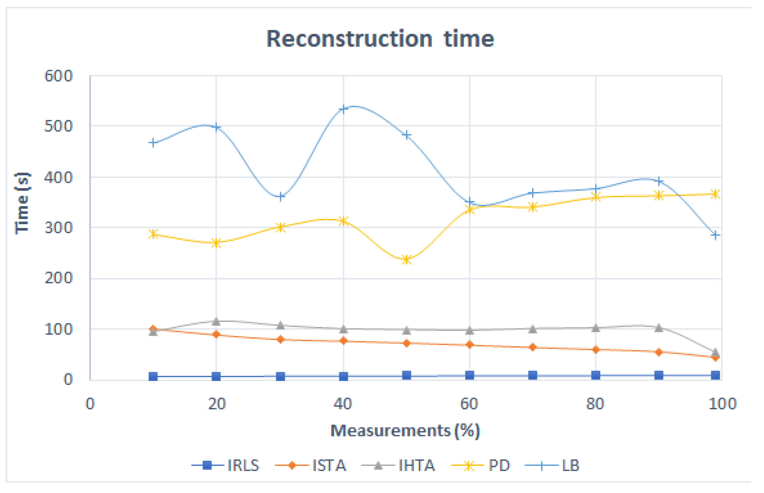
The graph in Figure 10 shows the time it takes for the algorithms to reconstruct the image based on the number of data entered. The IRLS maintains a constant time of 8 s in all reconstructions. It solves the rebuild problem in the norm and is the fastest. In the case of the ISTA, which employs a minimization in norm , the time decreases linearly from 100 s to approximately 50 s. The IHTA takes the longest time to rebuild, which is to be expected since it solves the minimization with the norm. In addition, two peaks are obtained at 20% and 90% of the measurements with IHTA. The convex algorithms, PD and LB, take much longer than the greedy ones as expected. The PD reconstruction time is longer, as the number of measurements increases. Its maximum value is 367 s. The LB algorithm does not show a clear trend. It has three peaks, at 20%, 40% and 90%, the latter being the softest. Finally, with 100%, the time is reduced to 285 s. Note that in general, the reconstruction time is not very important when reconstructing one or few images, so with respect to this factor, it would be beneficial to use the most accurate algorithm regardless of the time it takes.
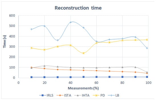
Figure 10.
Reconstruction time of Figure 3 as a function of the number of measurements for each algorithm.
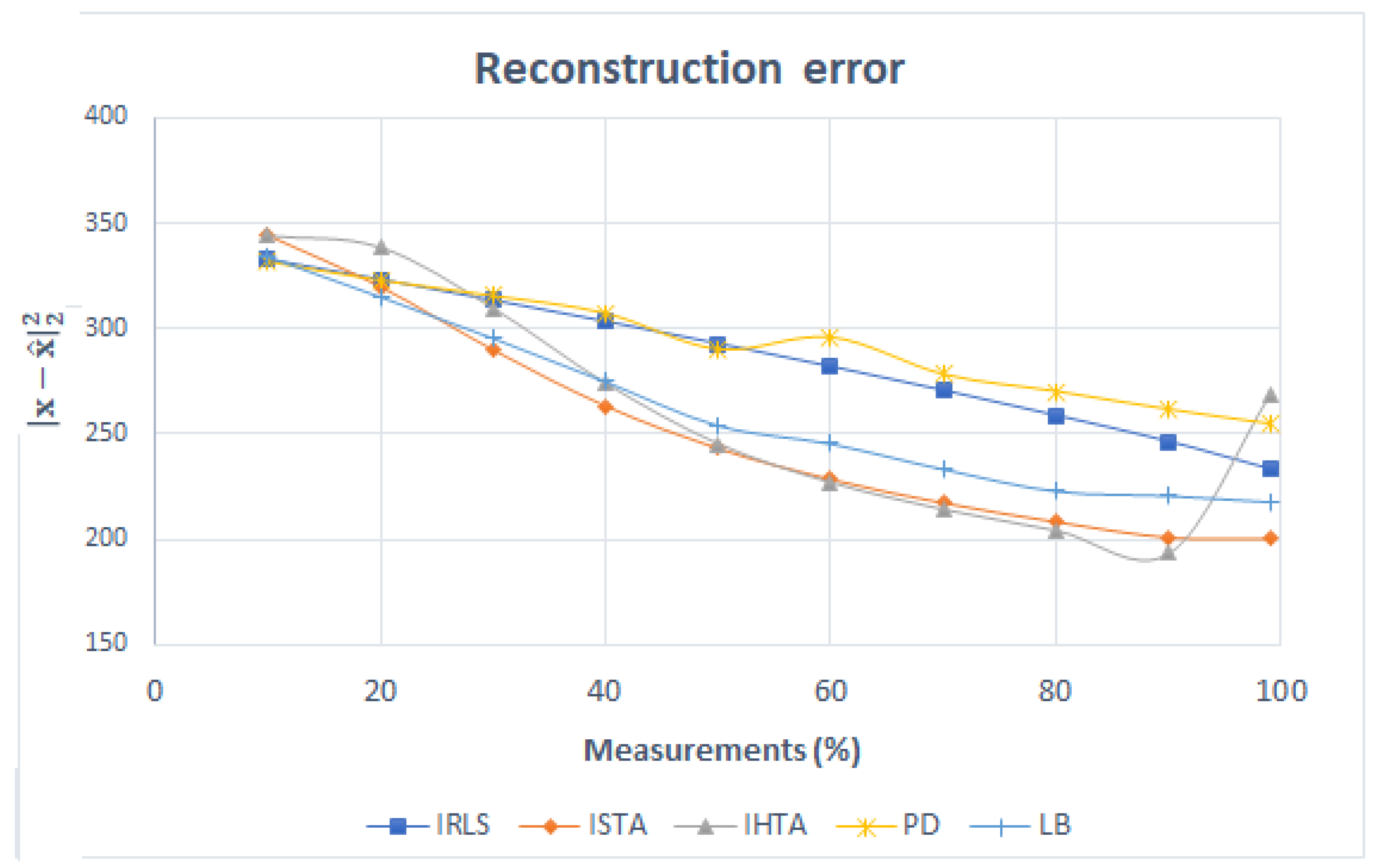
The error made in the reconstruction can be seen in the following Figure 11. The IRLS error decreases linearly. The trends in ISTA and IHTA are very similar: in both, the error decreases with the number of measurements. However, when 90% of the measurements is reached, the error with IHTA increases sharply. This is due to the fact that, as mentioned above, in the last reconstruction, the algorithm does not detect the signal related to the white matter and, therefore, returns a larger error. The error for PD and LB is higher than expected since they are convex algorithms, and the reconstructed images are quite similar to the original ones. Both algorithms decrease the error in a similar way up to 60%, where the error in PD is greater.
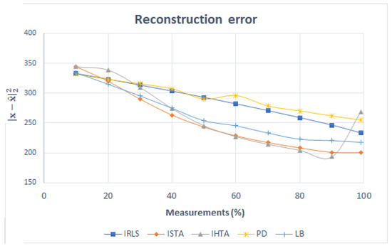
Figure 11.
Error in the reconstruction of Figure 3 as a function of the number of measurements for each algorithm.
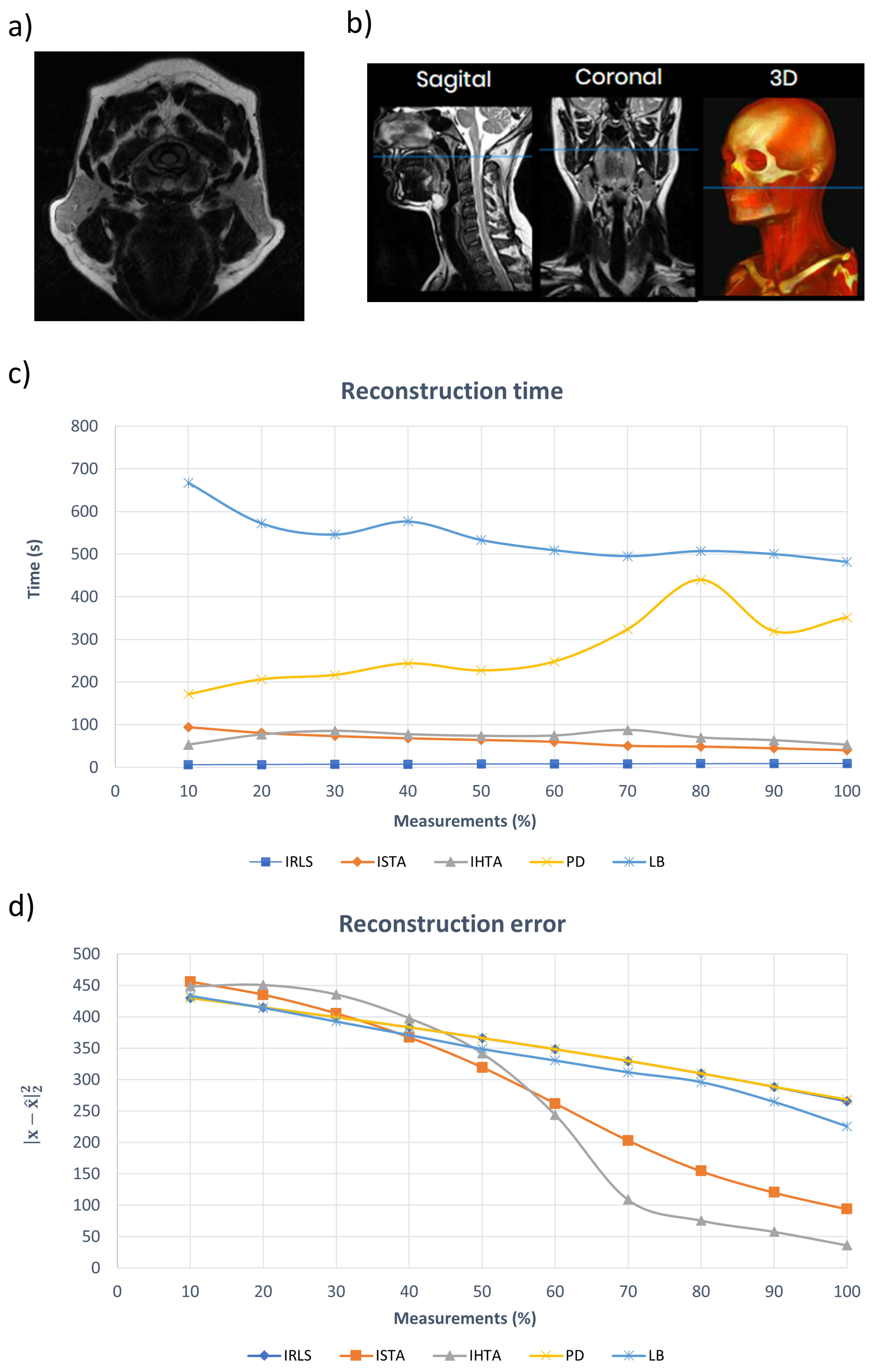
An additional analyzed image (Figure 12a) corresponds to the plane indicated by the blue lines in Figure 12b, representing an axial section. The region of the face and neck is presented. The black “U” shape at the bottom is the teeth, while the spinal cord is centrally located above them. Figure 12c,d illustrate the computation time and the reconstruction error of the algorithms, respectively. Both parameters show similar trends to those observed in the previous image. The LB algorithm exhibits the longest reconstruction time but achieves the lowest error when the amount of input data is small. However, as the size of the data set increases, the LB algorithm shows a larger error. PS has the second longest rebuild time, and its error is comparable to that of IRLS, which is the fastest algorithm. ISTA and IHTA show similar reconstruction times, with the latter showing the lowest error among all the algorithms.
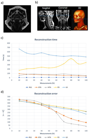
Figure 12.
(a) MRI image analyzed. (b) Images of sagittal, coronal and 3D slices of the head. The blue line shows the plane corresponding to (a). (c) Reconstruction time of (a) as a function of the number of measurements for each algorithm. (d) Error in the reconstruction of (a) as a function of the number of measurements for each algorithm.
Finally, possible limitations of the study and possible solutions should be addressed. First, the data set used may be somewhat specific to the field of MRI medical imaging, which has very similar colors and contrasts and all follow a very similar acquisition process with long exposure times, and it would be nice to check the applicability of the study to other types of medical images such as those taken for example with X-rays. Second, the algorithms, although of different origin and with different strengths and limitations, can be considered quite specific to the field of compressed detection and would be good to explore new possibilities, such as the use of different rules or mathematical concepts, which could lead to further improvements in the reconstruction process.
5. Conclusions
In this work, CS techniques applied to images acquired with magnetic resonance were studied. Several programs were developed that allowed us to reconstruct an image quickly and clearly. A random signal was started with a smaller number of data than those necessary to construct the original image in a conventional way. A similar image was then generated at a lower resolution. The algorithms chosen to perform this task were IRLS, ISTA, IHTA, PD and LB.
From the analysis of the images reconstructed with these algorithms, it can be concluded that it is appropriate to use ISTA. Although it has adequate computational time and in some cases may not give the best possible resolution, it allows distinguishing each component if 70% or more of the measurements are taken. Although the IHTA algorithm is the highest resolution, it does not correctly resolve some images and takes longer to perform the reconstruction. The IRLS algorithm has the shortest computational time, but, like IHTA, it does not achieve sufficient precision. If there is less than 50% of the measurements, the PD algorithm should be used since its images are clearer and it can recover the structures. Keep in mind, however, that the proper detection of health problems with such low-resolution images may be highly expert-dependent or would need to be assisted by statistical analysis. The LB algorithm takes too much time and does not offer any improvement compared to the other algorithms.
These algorithms can be applied to different parts of the human body and with different MRI sequences, such as , or proton density. These sequences change the contrast of the images, allowing a distinction to be made between the components of the human body. Images can also be reconstructed even if contrast agents are introduced.
The same CS technique studied in this article can be applied to other methods; for example, CT scan or X-ray. Although the acquisition time of these is much shorter, it can still reduce the amount of radiation applied to the human body needed to obtain an image.
Then, finally, the ISTA algorithm can be recommended as the most adequate to reconstruct magnetic resonance images with sufficient precision and computational efficiency. For cases where the exposure time can be very long and the process would benefit from fewer measurements (less than 50%), PD would be the best option. However, for other scenarios, such as images taken with less time (X-rays), the IHTA algorithm should be preferred, as it provides the highest accuracy.
Author Contributions
A.E.H.-A. developed part of the mathematical formalism and performed the compressed sensing calculations. V.M.G.-S. proposed the research, obtained the medical images and reviewed the article. J.L.F.-M. developed the mathematical formalism. All authors have read and agreed to the published version of the manuscript.
Funding
This research received no external funding.
Data Availability Statement
The data that support the findings of this study are available from the corresponding author upon reasonable request.
Conflicts of Interest
The authors declare no conflict of interest.
References
- Shannon, C. Communication in the Presence of Noise. Proc. IRE 1949, 37, 10–21. [Google Scholar] [CrossRef]
- Baraniuk, R.G.; Cevher, V.; Duarte, M.F.; Hegde, C. Model-Based Compressive Sensing. IEEE Trans. Inf. Theory 2010, 56, 1982–2001. [Google Scholar] [CrossRef]
- Donoho, D. Compressed sensing. IEEE Trans. Inf. Theory 2006, 52, 1289–1306. [Google Scholar] [CrossRef]
- Candès, E.; Romberg, J.; Tao, T. Robust uncertainty principles: Exact signal reconstruction from highly incomplete frequency information. IEEE Trans. Inf. Theory 2006, 52, 489–509. [Google Scholar] [CrossRef]
- Rani, M.; Dhok, S.B.; Deshmukh, R.B. A Systematic Review of Compressive Sensing: Concepts, Implementations and Applications. IEEE Access 2018, 6, 4875–4894. [Google Scholar] [CrossRef]
- Dwork, N.; O’Connor, D.; Baron, C.A.; Johnson, E.; Kerr, A.B.; Pauly, J.M.; Larson, P.E.Z. Utilizing the wavelet transform’s structure in compressed sensing. SIViP 2021, 15, 1407–1414. [Google Scholar] [CrossRef] [PubMed]
- Chen, Z.; Huang, C.; Lin, S. A new sparse representation framework for compressed sensing MRI. Knowl.-Based Syst. 2020, 188, 104969. [Google Scholar] [CrossRef]
- Geethanath, S.; Reddy, R.; Konar, A.; Imam, S.; Sundaresan, R.; Babu, D.R.R.; Vanketasan, R. Compressed Sensing MRI: A Review. Crit. Rev. Biomed. Eng. 2013, 41, 183–204. [Google Scholar] [CrossRef]
- Orovic, I.; Papic, V.; Ioana, C.; Li, X.; Stankovic, S. Compressive Sensing in Signal Processing: Algorithms and Transform Domain Formulations. Math. Probl. Eng. 2016, 2016, 7616393. [Google Scholar] [CrossRef]
- Majumdar, A. Compressed Sensing for Engineers; Taylor & Francis Group: Abingdon, UK, 2019. [Google Scholar]
- Ouyang, B.; Dalgleish, F.R.; Caimi, F.M.; Giddings, T.E.; Shirron, J.J.; Vuorenkoski, A.K.; Nootz, G.; Britton, W.; Ramos, B. Underwater laser serial imaging using compressive sensing and digital mirror device. In Laser Radar Technology and Applications XVI: 27–29 April 2011, Orlando, Florida, United States; Turner, M.D., Kamerman, G.W., Eds.; International Society for Optics and Photonics, SPIE: Bellingham, DC, USA, 2011; Volume 8037, pp. 67–77. [Google Scholar]
- Zou, Z.; Bao, Y.; Li, H.; Spencer, B.F.; Ou, J. Embedding Compressive Sensing-Based Data Loss Recovery Algorithm Into Wireless Smart Sensors for Structural Health Monitoring. IEEE Sens. J. 2015, 15, 797–808. [Google Scholar] [CrossRef]
- Torruella, P.; Arenal, R.; de la Peña, F.; Saghi, Z.; Yedra, L.; Eljarrat, A.; López-Conesa, L.; Estrader, M.; López-Ortega, A.; Salazar-Alvarez, G.; et al. 3D Visualization of the Iron Oxidation State in FeO/Fe3O4 Core–Shell Nanocubes from Electron Energy Loss Tomography. Nano Lett. 2016, 16, 5068–5073. [Google Scholar] [CrossRef] [PubMed]
- Dance, D.; Christofides, S.; Maidment, A.; McLean, I.; Ng, K. Diagnostic Radiology Physics: A Handbook for Teachers and Students; IAEA: Vienna, Austria, 2014. [Google Scholar]
- Laboratory of Neuro Imaging. LONI Image Data Archive (IDA). 2021. Available online: https://ida.loni.usc.edu (accessed on 1 May 2021).
- The Centre for Phenogenomics. MICe Mouse Imaging Centre. 2004. Available online: http://www.mouseimaging.ca/index.html (accessed on 1 May 2021).
- López Larrubia, P. Aplicaciones de la resonancia magnética nuclear a la investigación biomédica. In Proceedings of the SEBBM Divulgación, Oviedo, Spain; 2009. [Google Scholar]
- Dawson, M. Paul Lauterbur and the Invention of MRI; MIT Press: Cambridge, MA, USA, 2013. [Google Scholar]
- Martínez Guillamón, C. Aplicaciones Clínicas y Protocolos de Actuación en Resonancia Magnética; Galindo, S.L., Ed.; Asociación Española de Técnicos de Radiología: Madrid, Spain, 2008. [Google Scholar]
- Lustig, M.; Donoho, D.; Pauly, J. Sparse MRI: The application of compressed sensing for rapid MR imaging. IEEE Trans. Signal Process. 2007, 58, 1182–1195. [Google Scholar] [CrossRef] [PubMed]
- Smith, A.; Johnson, C.; Williams, J. Accelerated MRI Reconstruction using Iterative Re-Weighted Least Squares. IEEE Trans. Med. Imaging 2007, 34, 2299–2312. [Google Scholar]
- Daubechies, I.; Defrise, M.; De Mol, C. An iterative thresholding algorithm for linear inverse problems with a sparsity constraint. Commun. Pure Appl. Math. 2004, 57, 1413–1457. [Google Scholar] [CrossRef]
- Blumensath, T.; Davies, M. Iterative hard thresholding for compressed sensing. Appl. Comput. Harmon. Anal. 2008, 27, 265–274. [Google Scholar] [CrossRef]
- Chambolle, A.; Pock, T. A first-order primal-dual algorithm for convex problems with applications to imaging. J. Math. Imaging Vis. 2011, 40, 120–145. [Google Scholar] [CrossRef]
- Zhu, H.; Zhang, Y.; Li, X. A Novel Primal Dual Algorithm for MRI Reconstruction. In Proceedings of the Annual International Conference of the IEEE Engineering in Medicine and Biology Society, Berlin, Germany, 23–27 July 2019; pp. 2589–2592. [Google Scholar]
- Kim, K.; Koh, K.; Lustig, M.; Boyd, S.; Gorinevsky, D. An interior-point method for large-scale l1-regularized least squares. IEEE J. Sel. Top. Signal Process. 2007, 1, 606–617. [Google Scholar] [CrossRef]
- Badnjar, J. Comparison of Algorithms for Compressed Sensing of Magnetic Resonance Images. arXiv 2015, arXiv:1502.02182. [Google Scholar]
- Sher, Y. Review of Algorithms for Compressive Sensing of Images. arXiv 2019, arXiv:1908.01642. [Google Scholar]
- Yu, Y.; Hong, M.; Liu, F.; Wang, H.; Crozier, S. Comparison and analysis of nonlinear algorithms for compressed sensing in MRI. In Proceedings of the 2010 Annual International Conference of the IEEE Engineering in Medicine and Biology, Buenos Aires, Argentina, 31 August–4 September 2010; pp. 5661–5664. [Google Scholar] [CrossRef]
- Wang, Z.; Gao, Y.; Duan, X.; Cao, J. Adaptive High-Resolution Imaging Method Based on Compressive Sensing. Sensors 2022, 22, 8848. [Google Scholar] [CrossRef]
- Zhao, W.; Gao, L.; Zhai, A.; Wang, D. Comparison of common algorithms for Single-Pixel Imaging via Compressed Sensing. Sensors 2023, 23, 4678. [Google Scholar] [CrossRef] [PubMed]
- Hammernik, K.; Klatzer, T.; Kobler, E.; Recht, M.P.; Sodickson, D.K.; Pock, T.; Knoll, F. Learning a variational network for reconstruction of accelerated MRI data. Magn. Reson. Med. 2018, 79, 3055–3071. [Google Scholar] [CrossRef] [PubMed]
- Machidon, A.L.; Pejovic, V. Deep learning for compressive sensing: A ubiquitous systems perspective. Artif. Intell. Rev. 2023, 56, 3619–3658. [Google Scholar] [CrossRef]
- Griswold, M.A.; Jakob, P.M.; Heidemann, R.M.; Nittka, M.; Jellus, V.; Wang, J.; Kiefer, B.; Haase, A. Generalized autocalibrating partially parallel acquisitions (GRAPPA). Magn. Reson. Med. 2002, 47, 1202–1210. [Google Scholar] [CrossRef]
- Mallat, S. A Wavelet Tour of Signal Processing, Third Edition: The Sparse Way, 3rd ed.; Academic Press, Inc.: Cambridge, MA, USA, 2008. [Google Scholar]
- Elahi, S.; Kaleem, M.; Omer, H. Compressively sampled MR image reconstruction using generalized thresholding iterative algorithm. J. Magn. Reson. 2018, 286, 91–98. [Google Scholar] [CrossRef]
- Beck, A.; Teboulle, M. A fast Iterative Shrinkage-Thresholding Algorithm with application to wavelet-based image deblurring. In Proceedings of the 2009 IEEE International Conference on Acoustics, Speech and Signal Processing, Taipei, Taiwan, 19–24 April 2009; pp. 693–696. [Google Scholar] [CrossRef]
- Tan, Z.; Eldar, Y.; Beck, A.; Nehorai, A. Smoothing and Decomposition for Analysis Sparse Recovery. IEEE Trans. Signal Process. 2014, 62, 1762–1774. [Google Scholar] [CrossRef]
- Liu, Y.; Zhan, Z.; Cai, J.; Guo, D.; Chen, Z.; Qu, X. Projected Iterative Soft-Thresholding Algorithm for Tight Frames in Compressed Sensing Magnetic Resonance Imaging. IEEE Trans. Med. Imaging 2016, 35, 2130–2140. [Google Scholar] [CrossRef] [PubMed]
- Zibetti, M.; Helou, E.; Regatte, R.; Herman, G. Monotone FISTA With Variable Acceleration for Compressed Sensing Magnetic Resonance Imaging. IEEE Trans. Comput. Imaging 2019, 5, 109–119. [Google Scholar] [CrossRef]
- Zhang, G.; Deng, H.; Chen, Y. Investigating the stability of fast iterative shrinkage thresholding algorithm for MR imaging reconstruction using compressed sensing. In Proceedings of the 2015 12th International Conference on Fuzzy Systems and Knowledge Discovery (FSKD), Zhangjiajie, China, 15–17 August 2015; pp. 1296–1300. [Google Scholar] [CrossRef]
- Boyd, S.; Vandenberghe, L. Convex Optimization; Cambridge University Press: Cambridge, UK, 2014. [Google Scholar]
- Candès, E.; Romberg, J. l1-MAGIC. Recovery of Sparse Signals via Convex Programming. 2005. Available online: https://candes.su.domains/software/l1magic/downloads/l1magic.pdf (accessed on 1 May 2021).
- Sartori, P.; Rozowykniat, M.; Siviero, L.; Barba, G.; Peña, A.; Mayol, N.; Acosta, D.; Castro, J.; Ortiz, A. Artefactos y artificios frecuentes en tomografía computada y resonancia magnética. Rev. Argent. Radiol. 2015, 79, 192–204. [Google Scholar] [CrossRef]
Disclaimer/Publisher’s Note: The statements, opinions and data contained in all publications are solely those of the individual author(s) and contributor(s) and not of MDPI and/or the editor(s). MDPI and/or the editor(s) disclaim responsibility for any injury to people or property resulting from any ideas, methods, instructions or products referred to in the content. |
© 2023 by the authors. Licensee MDPI, Basel, Switzerland. This article is an open access article distributed under the terms and conditions of the Creative Commons Attribution (CC BY) license (https://creativecommons.org/licenses/by/4.0/).

