Abstract
This paper discusses using unsupervised learning in classifying particle-like dispersion. The problem is relevant to various applications, including virus transmission and atmospheric pollution. The Reduce Uncertainty and Increase Confidence (RUN-ICON) algorithm of unsupervised learning is applied to particle spread classification. The algorithm classifies the particles with higher confidence and lower uncertainty than other algorithms. The algorithm’s efficiency remains high also when noise is added to the system. Applying unsupervised learning in conjunction with the RUN-ICON algorithm provides a tool for studying particles’ dynamics and their impact on air quality, health, and climate.
Keywords:
unsupervised learning; machine learning; artificial intelligence; particles dispersion; virus transmission; air quality; atmospheric pollution MSC:
68T20
1. Introduction
Unsupervised learning (UL) has been established as a machine learning (ML) approach that eliminates human bias from the analysis [1,2,3]. We could also take it one step further and claim that UL can be used to reduce computational bias or reduce the uncertainty associated with numerical algorithms and processes. The computational groups are not defined by the researcher but by the algorithm. UL could be better suited for problems of higher complexity in identifying the groups. Moreover, it is easier to obtain unlabelled data—experimental, computational or field measurements—than labelled data that require user intervention. UL could be more difficult because no labels are pre-defined.
The motivation for this work emanates from two diverse applications, namely, virus transmission and atmospheric pollution. In these applications, knowing how particles are dispersed in space and time according to defined properties would be important. It could help identify particle transmission properties and establish patterns based on distinctive properties such as weight and size. Particle simulations associated with virus transmission and atmospheric pollution are computationally expensive, including the post-processing effort required in analysing the particle’s behaviour. UL models can provide a useful tool in classifying particle dispersion through clustering. We outline below in further detail how UL could be useful in the above two applications. Still, there are many other areas where particle dispersion is relevant, including pharmaceuticals, combustion engines, agriculture, food processing, biomedical and marine engineering.
Since the COVID-19 pandemic started, there has been a vast debate about virus transmission indoors and outdoors [4,5,6]. Computational modelling provides an alternative approach to simulating airborne virus transmission. The above was shown through several recent studies since the start of the pandemic [7,8,9,10,11,12,13]. The risk of airborne virus transmission indoors is higher than outdoors [4,14].
At the onset of this crisis, research studies demonstrated that the two metres of social distancing when people cough or sneeze is insufficient to protect people in the environment. It was shown that this is even more true when people are exposed to wind outdoors or flow circulation indoors due to an air conditioning system, which will disperse particles even further away. Note that the World Health Organization (WHO) advised 2 m of social distancing everywhere, indoors and outdoors, at that time. Although the aforementioned studies shed light on the virus transmission issues and elucidated many fundamental questions, it is complex to simulate a virus in real time and classify where the particles will land. In that case, UL could be used to identify higher-risk scenarios and guide solutions for risk reduction. For example, in an indoor space such as a school, office, hospital, or ship, one could experiment with various scenarios of virus onset and classify the areas more prone to receive the expelled from human particles. This could help decision-making about evacuation or space design arrangements to reduce the risk of transmission. Classification of particle-carrying virus dispersion is a complex problem depending on the environmental conditions, i.e., temperature and relative humidity. UL will not provide the precise locations but will show the spatial locations where particles disperse depending on their size. In other words, it will map out the dispersion envelope by simplifying the fluid dynamics complexity and providing a reduced-order model.
Dispersion of pollutants is another complex problem that depends on many environmental and atmospheric parameters [15,16]. Computational fluid dynamics (CFD), in conjunction with atmospheric models, can be used to simulate the dispersion of particles into the atmosphere [17,18]. Moreover, CFD simulates pollution in cities and other landscapes and indoor pollutants dispersion [19]. These problems are highly dependent on the initial condition. Real-time simulations would be expensive and require sensors to provide initial data for the simulations and assimilate field data during the execution of the simulations. Therefore, the applicability of simulations will be limited in real-time [20,21]. UL could classify pollutants dispersion in terms of location, size and chemical composition without resorting to expensive simulations that require high-performance computing facilities and complex, specialised computational software that, in turn, require dedicated human resources having the expertise to initialise the data, perform the simulations and post-process the results [22,23]. In some special cases, for example, pollution from aircraft and rockets, dispersion detection is extremely difficult due to the rapid release of exhaust gases [24].
Machine learning methods for particle dispersion have been proposed in the literature [25,26,27]. Some efforts concern the development of hybrid systems based on the combination of Unsupervised Clustering, Artificial Neural Networks (ANN), Random Forest (RF) and fuzzy logic to predict multiple criteria for pollutants. However, to our knowledge, there has not been a UL algorithm similar to the one presented here that can be universally applied to particle clustering. The specific contribution of the proposed RUN-ICON algorithm is discussed further in this paper.
This paper aims to present the UL algorithm RUN-ICON for a generalised, simple mathematical set-up mimicking particle dispersion. Future studies will focus on applying the algorithm to specific problems of virus transmission and atmospheric pollutants, and this work is underway. This paper is organised as follows. Section 2 briefly outlines the methods and issues we try to elucidate through numerical experiments. Section 3 presents the particle dispersion model. Section 4 presents the results from various numerical experiments. Conclusions are drawn in Section 5.
2. Materials and Methods
UL represents a fundamental machine learning paradigm that has persistently endured over the years and continues to hold paramount significance in diverse domains of research and applications, such as image processing [28,29], sleep stages classification [30] and mechanical damage detection [31]. When trying to apply UL to particle clustering, algorithms, such as K-means [32], hierarchical clustering [33], DBSCAN [34] and various deep learning-based approaches like autoencoders [35] and variational autoencoders [36] may prove instrumental in grouping particles with similar characteristics, based solely on their intrinsic features. They excel at discovering underlying patterns and structures within the data without needing pre-defined labels. Supervised learning techniques have been successfully applied in air particle analysis so far [37,38]. However, it is believed that since UL techniques are particularly well-suited for uncovering inherent patterns and structures present within data sets, such techniques may be applied to particle dispersion problems and efficiently identify distinct particle clusters based on size, composition or other relevant attributes.
2.1. Existing Challenges
UL algorithms, while powerful and versatile, do face significant challenges when it comes to particle clustering tasks:
- Ambiguous cluster boundaries: Unsupervised clustering algorithms, such as K-means or hierarchical clustering, rely on distance metrics to determine cluster boundaries. Defining unambiguous cluster boundaries can be challenging for particles with complex spatial distributions or overlapping clusters. Consequently, the algorithm may struggle to accurately separate and identify distinct particle clusters.
- Sensitivity to hyperparameters: Many unsupervised clustering algorithms require the specification of hyperparameters, such as the number of clusters (k) in K-means. Selecting the optimal value for these hyperparameters can be difficult, and the results may vary significantly based on these choices. Incorrect parameter selection can lead to poor clustering results and may require a trial-and-error approach.
- Dimensionality and feature selection: Particle data often contain many dimensions representing various physical properties of the particles. Unsupervised algorithms can face difficulties in handling high-dimensional data, as it can result in the curse of dimensionality [39]. Additionally, choosing the correct features that represent meaningful characteristics of the particles is crucial, and poor feature selection can impact clustering performance.
- Cluster shape and size variability: Unsupervised clustering algorithms typically assume that clusters have certain predefined shapes. In particle clustering tasks, clusters can have irregular shapes and varying sizes, which may not align with these assumptions. Consequently, the algorithm may struggle to represent the particle distributions’ inherent structure accurately.
- Robustness to noise: Particle data can be prone to noise and outliers due to measurement errors or other factors. Unsupervised clustering algorithms can be sensitive to noise, creating spurious clusters or inaccuracies in the clustering results.
- Limited supervision: In certain cases, some available supervision or domain knowledge about the particles could help improve clustering accuracy. Unsupervised algorithms, by definition, do not incorporate such external guidance, potentially missing out on valuable information that could aid in better clustering.
- Scalability: Some unsupervised clustering algorithms can become computationally expensive as the data set increases. Handling large-scale particle data sets efficiently can be challenging due to memory and processing limitations.
For further discussion on some of these limitations, the reader is referred to [40].
2.2. Contribution to Unsupervised Learning Advancement
The RUN-ICON algorithm [40] aims to address many of these challenges by ensuring the selection of the most dominant clusters occurs with high confidence and low uncertainty. The RUN-ICON was developed to avoid deciding on the optimum number of clusters based only on intuitive criteria. Instead, it effectively determines the optimal number of clusters by identifying commonly dominant centres across multiple repetitions of the K-means++ algorithm. The algorithm does not rely on the Sum of Squared Errors and determines optimal clustering by introducing novel metrics such as the Clustering Dominance Index (CDI) and Uncertainty. CDI is linked with the frequency of occurrence of a specific clustering configuration when requesting the splitting of the data set in a certain number of clusters and could be translated as the probability of that specific configuration occurring. Uncertainty is the relative difference between upper and lower CDI bounds for a clustering configuration and represents the maximum variance from the mean for that specific configuration. The superiority of RUN-ICON over different UL algorithms under different scenarios has been demonstrated in [40]. In this work, comparisons of RUN-ICON with other UL algorithms for the specific particle dispersion problem will also be given to demonstrate the superiority of our method over these techniques. These algorithms include commonly utilized techniques, such as:
- Repeat K-means [41]: This is a modified version of the traditional K-means that focuses on improving clustering results by iteratively refining the initial cluster centres through a process of perturbation and reassignment, leading to more stable and reliable clusters in the presence of noisy data or uncertain initialization.
- Bayesian K-means [42]: This method extends the traditional K-means clustering algorithm incorporating Bayesian inference principles to provide a more flexible and probabilistic approach to clustering.
- DBSCAN [34]: Density-Based Spatial Clustering of Applications with Noise (DBSCAN) is a clustering algorithm that groups closely packed data points in a data set based on their density. It identifies clusters by defining dense regions separated by sparser regions and can find arbitrarily shaped clusters while also identifying noise points that do not belong to any cluster.
In the following section, a simplified model for particle dispersion is given, and a series of numerical experiments are performed with and without noise, demonstrating the algorithm’s capacity to effectively differentiate particles into distinct clusters, relying initially on their final spatial distributions.
3. A Simplified Particle Dispersion Problem
This paper presents a numerical experiment to evaluate the RUN-ICON algorithm’s ability to represent the collective behaviour of a group of non-interacting particles originating from a common point. These particles are left to propagate following a set of ordinary differential equations, allowing multiple particles to follow the same trajectory. The primary objective is to assess the algorithm’s capacity to capture the complex dynamics exhibited by the particle group and its potential applications in simulating particle-based systems without the need for computationally expensive inter-particle force calculations. The set of equations used to simulate the particle trajectories are:
with initial conditions , . This system has analytical solutions of the form:
and is solved for 10 time units, with a timestep of . Initial values are all taken to be zero. It has to be mentioned that time and space are taken as dimensionless. In this study, artificial data were generated using the above model to showcase the capability of the RUN-ICON algorithm to discriminate among particles under diverse conditions during their stochastic spatial dispersion. If the algorithm demonstrates proficiency, achieving successful outcomes in scenarios involving dissimilar attributes in data sets, such as distinct temperatures, humidities, sizes, chemical compositions, collection locations, etc., could become considerably more attainable.
The following section presents simulation results with and without noise in the solution.
4. Results
4.1. Particle Dispersion When No Noise Is Added
Initially, the model follows the trajectories of 1000 particles in space and time when no noise is present, and all particles follow the trajectories described by Equations (3) and (4). The number 1000 was chosen as representative of the order of magnitude of particles that are emitted during the coughing of a person [43] and the possible transmission of viruses. The trajectories in the dimensionless x-y plane are depicted in Figure 1 for c’s and d’s varying randomly within the range (a) (0, 0.1), (b) (0, 0.5) and (c) (0, 1.0), (generated by a uniform random number generator). As observed, the behaviour of particles in the three tests differs depending on the range of parameters c and d. When c’s and d’s were small, the particles did not have the time to travel far away from the origin, thus exhibiting a uniform dispersion in all positive x and y directions. As parameters c and d increase, particle separation occurs, with the particles being biased to travel mostly along the positive x or y axes. This separation becomes more pronounced when parameters c and d obtain values from the range (0, 1.0). Obviously, because of the exponential dependence of the solution, the final distances covered by the particles are not proportional to how c’s and d’s increase.

Figure 1.
Trajectories for 1000 particles in the dimensionless x-y plane with parameters varying randomly between (a) 0 and 0.1, (b) 0 and 0.5 and (c) 0 and 1.0. Each line represents the trajectory of a single particle. The colours assigned to the lines serve the purpose of discretising trajectories for individual particles.
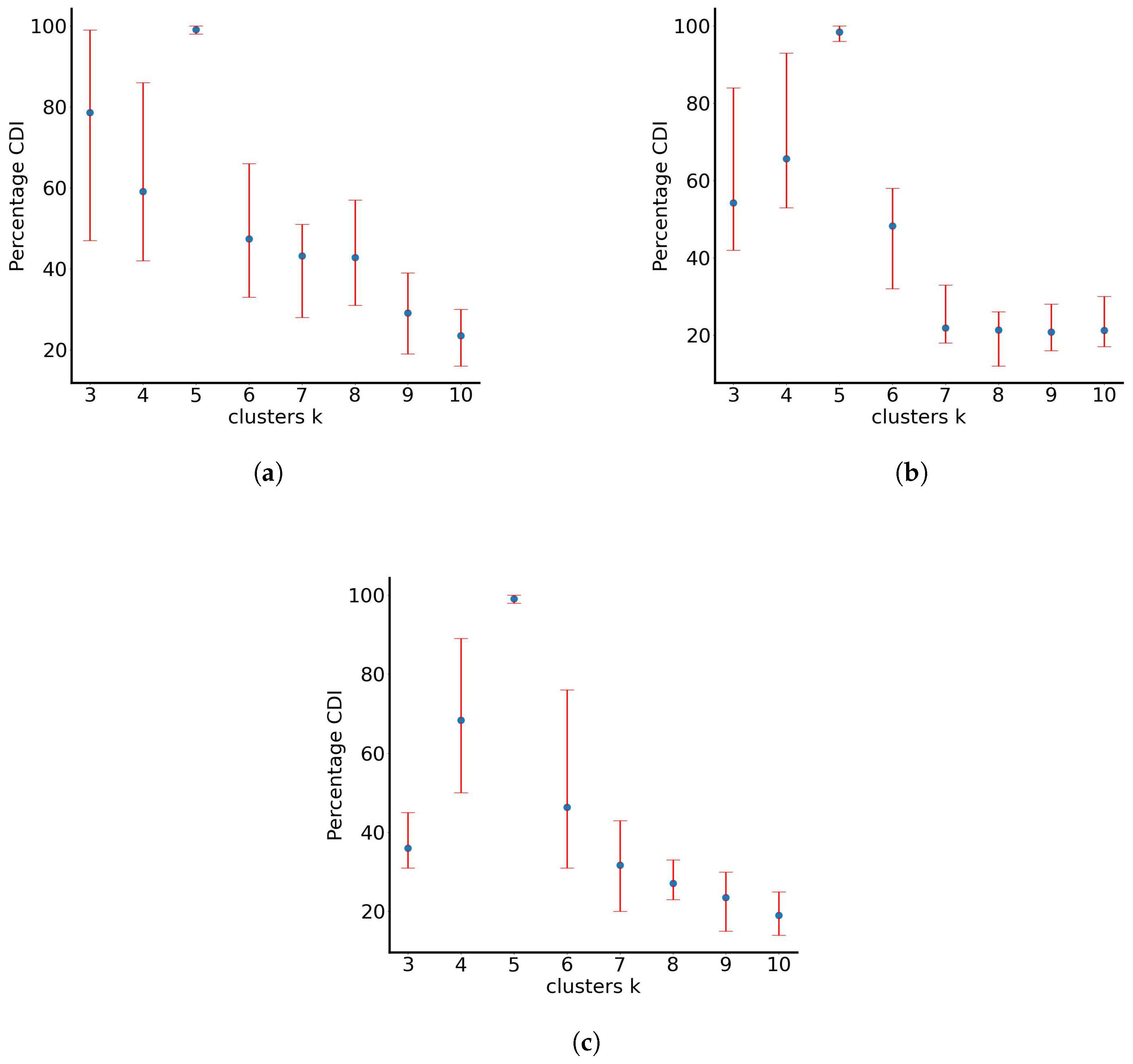
RUN-ICON is utilised on the normalised data sets of the final particle positions. In Figure 2, the results of clustering using the RUN-ICON algorithm are presented, where the highest average CDI (defined in [40]) and its upper and lower bounds (which define Uncertainty, as defined in [40]) are presented for clustering the data from 3 to 10 clusters. We consider clustering from three clusters and above, as discussed in [40]. The optimal clustering and the respective average highest CDI and uncertainty for all three test cases are presented in Table 1. From the presented results, it becomes clear that clustering the particles initially in four groups ((a), when they have not travelled far from the origin) and then in three groups ((b) and (c), when they travel further away) is optimal. The difference between the highest and the second-best CDI for all three cases ranges up to almost 50%, with the respective uncertainties (for the second-best CDI) being quite high (up to almost 0.4).
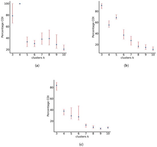
Figure 2.
Percentage averaged CDI for particles with parameters varying randomly between (a) 0 and 0.1, (b) 0 and 0.5 and (c) 0 and 1.0.

Table 1.
Performance of the RUN-ICON algorithm during particle dispersion when parameters c and d vary between (a) 0 and 0.1, (b) 0 and 0.5 and (c) 0 and 1.0.
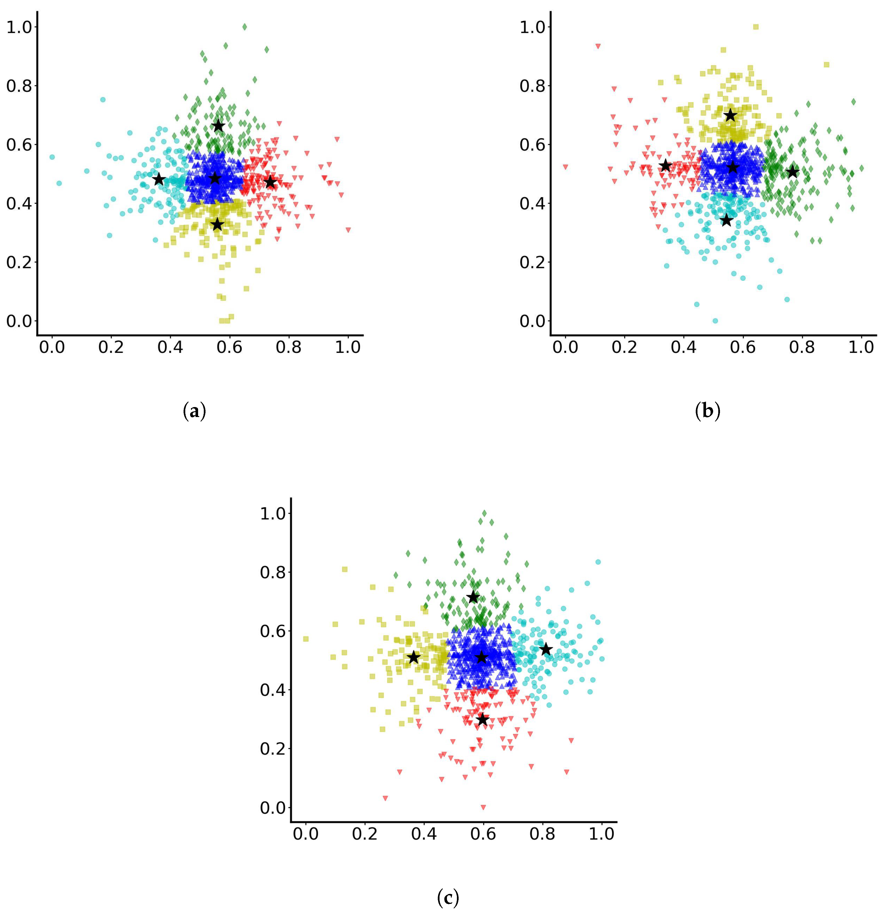
Then, based on the final position of particles (after 10-time units), the clustering is presented on the normalised data sets in Figure 3. As observed, for case (a), the particles are separated into four, almost square, clusters. The algorithm, when particles have not travelled far from the origin, manages to detect particles that are concentrated around the origin, particles that have travelled away from the origin in both positive x and y directions, particles that travel away from the origin only along the positive x direction and particles travelling away from the origin only along the positive y direction. Then for cases (b) and (c), it seems that separation in 3 clusters is optimal, where some particles have travelled along the positive x axis away from the origin, some others have travelled along the positive y axis away from the origin, and a third group have not managed to travel far and have remained concentrated around the origin. As the results show, the more the range of variation for parameters c and d increases, the more distinct the separation in three groups becomes.
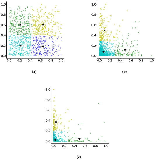
Figure 3.
Dominant clustering of particles with parameters varying randomly between (a) 0 and 0.1, (b) 0 and 0.5 and (c) 0 and 1.0. The stars indicate the cluster centres. Different colours indicate different clusters.
Then, the three clustering experiments were repeated with repeat K-means and Bayesian K-means and their clustering efficiencies (using the Silhouette Coefficient (SC) [44]) were determined. The results appear in Table 2, Table 3 and Table 4, for the three different test cases, where parameters c and d vary within the range (0, 0.1), (0, 0.5) and (0, 1.0), respectively.
Table 2.
Clustering efficiency of repeat and Bayesian K-means algorithms when parameters c and d vary between 0 and 0.1.
Table 3.
Clustering efficiency of repeat and Bayesian K-means algorithms when parameters c and d vary between 0 and 0.5.
Table 4.
Clustering efficiency of repeat and Bayesian K-means algorithms when parameters c and d vary between 0 and 1.0.
In Table 2, it may be observed that repeat K-means attains marginally the highest SC when using four clusters. However, it is noteworthy that the SC remains consistently low across clusterings from 3 to 10 clusters. This implies that the algorithm encounters considerable challenges in discerning the optimal clustering solution among these configurations. Bayesian K-means faces similar difficulties, with the partitioning into four clusters being marginally the most favourable outcome.
The results in Table 3 indicate that the repeat K-means algorithm achieves the highest SC of 0.60 when partitioning the data into three clusters. Moreover, all SC values are between 0.45 and 0.60 across various clusterings from 3 to 10 clusters, indicating the algorithm’s difficulty in distinguishing the optimal clustering solution. In contrast, Bayesian K-means suggests that a four-cluster partitioning is an optimal choice (with not very high SC), diverging from the predictions of RUN-ICON and repeat K-means methods.
As observed in Table 4, the repeat K-means algorithm faces increasing challenges in identifying the optimal clustering solution, as evidenced by all SCs being higher than 0.61 for various cluster configurations. This indicates the algorithm’s limited ability to distinguish the most suitable partitioning in the data. On the other hand, the Bayesian K-means algorithm predicts that the optimal clustering entails a separation into four distinct clusters, which differs from the clustering predictions of both other methods (i.e., RUN-ICON and repeat K-means).
Moreover, the DBSCAN algorithm was applied to the normalised data of all three test cases with different combinations of , i.e., the maximum distance between two points for them to be considered as part of the same neighbourhood, and , i.e., the minimum number of data points required to form a dense region in the clustering process). The result was that the algorithm failed to find multiple clusters for any combination. The hyperparameters of the DBSCAN algorithm, and , took values from the sets (0.1, 0.3, 0.5, 0.7) and (5, 10, 15), respectively.
These contrasting clustering behaviours underscore the complexity of the data and the sensitivity of clustering outcomes to the selected algorithms. Only RUN-ICON predicts clustering with high confidence and low uncertainty, indicating the algorithm’s ability and potential to produce robust clustering results in complex data sets.
It should be noted at this point that the time the Bayesian K-means algorithm takes to run is more than twice that of the other methods. This is a known disadvantage of the algorithm, and there are several reasons: The Bayesian K-means algorithm uses Gibbs sampling to approximate the posterior distribution of the cluster centres. Gibbs sampling involves iteratively sampling from conditional distributions, which can be computationally expensive compared to the simple update step in conventional K-means. Moreover, the algorithm estimates the covariance matrices for each cluster. This involves computing inverse matrices and performing additional matrix operations, which can be time-consuming, especially when dealing with large or high-dimensional data sets. Finally, the algorithm often requires more iterations to converge compared to standard K-means. The additional iterations increase the overall computational time. For a thorough discussion on Bayesian clustering analysis, the interested reader is referred to [45].
4.2. Particle Dispersion with Added Noise
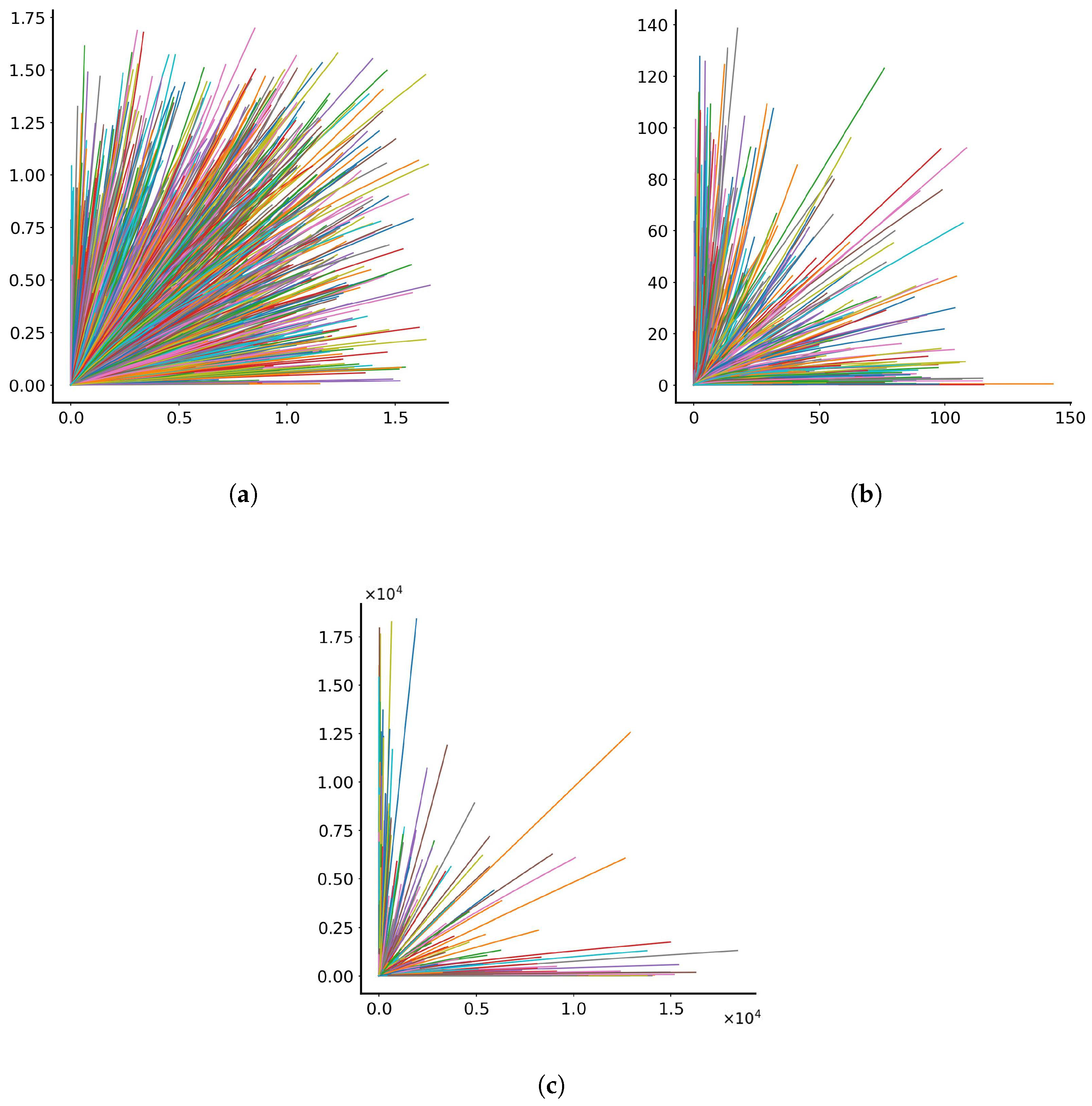
Further, noise is applied directly to the solution in the form of where t is the current time and is a normal distribution with mean equal to zero and standard deviation equal to . The experiment is repeated with varying randomly between 0 and 0.1, 0 and 0.5 and 0 and 1.0. It was observed that in all previous experiments, the noise term seemed to dominate, and all performed experiments (nine in total, considering the three ranges within which parameters c and d were allowed to vary randomly) displayed similar behaviour, except one, which will be discussed later. Thus, it was decided to examine with noise only the case with c’s and d’s varying randomly between (0, 0.1). The particle trajectories in the dimensionless x-y plane for each of the three experiments where the noise was applied to are shown in Figure 4.
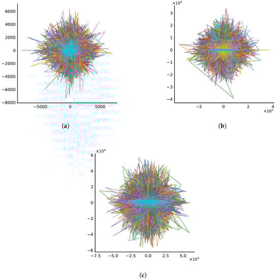
Figure 4.
Trajectories of 1000 particles in the dimensionless x-y plane with noise standard deviation varying randomly between (a) 0 and 0.1, (b) 0 and 0.5 and (c) 0 and 1.0. Each line represents the trajectory of a single particle. The colours assigned to the lines serve the purpose of discretising trajectories for individual particles.
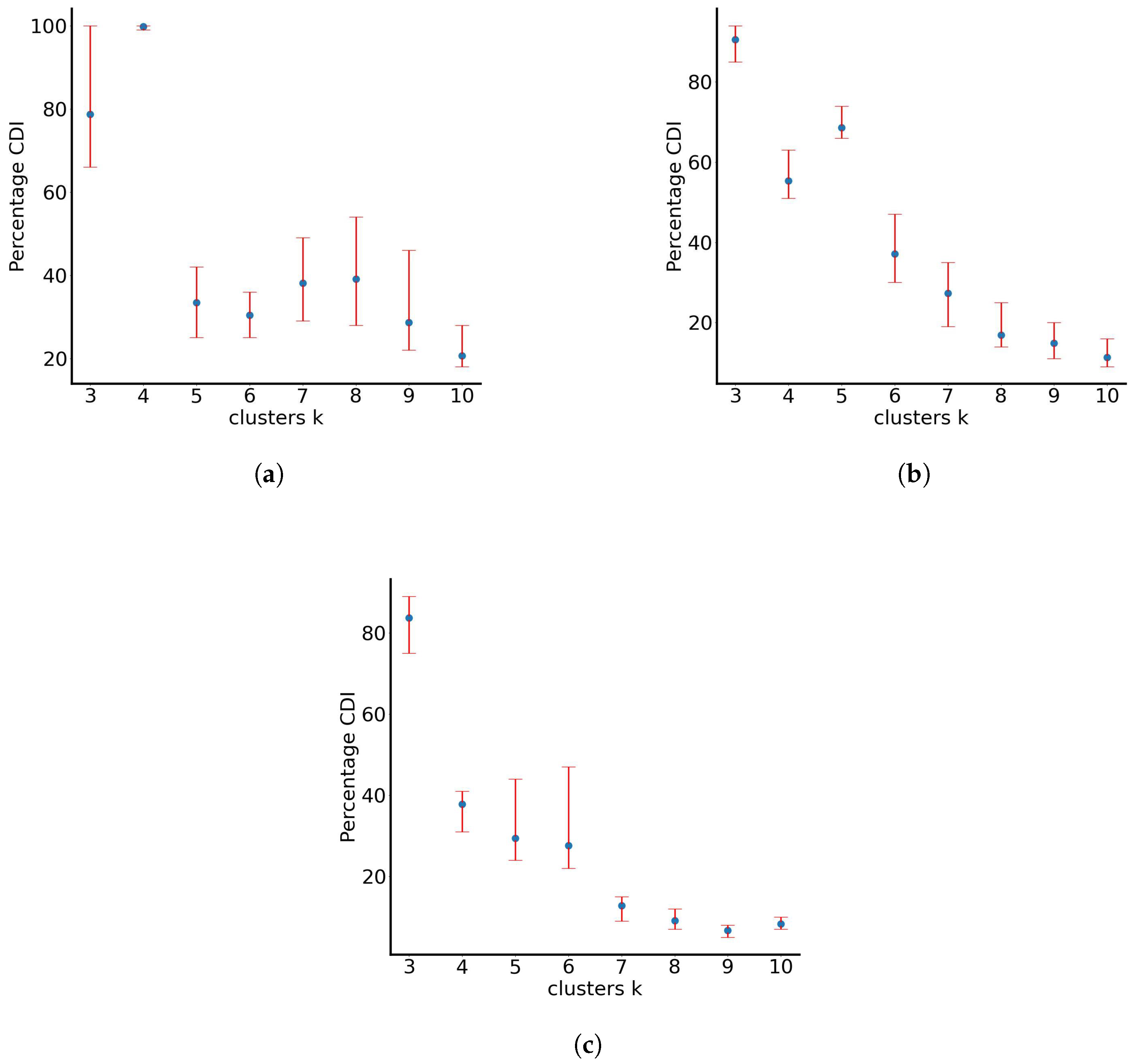
In this case, the behaviour is markedly different, with particles zig-zagging and forming rhomboid-like shapes around the origin (0, 0), extending towards positive and negative values in the x and y axes. The distances travelled by particles between the three test cases seem to be proportional to the standard deviation of noise: particles having a standard deviation up to 0.1 have travelled distances up to 8000 spatial units away from the origin; particles having a standard deviation up to 0.5 have travelled distances up to 40,000 spatial units away from the origin; and particles having standard deviation up to 1.0 have travelled distances over to 50,000 spatial units away from the origin. Once again, RUN-ICON is utilised on the normalised data sets of the final particle positions. Figure 5 presents the results of the RUN-ICON algorithm, where the highest average CDI and its upper and lower bounds are presented for clustering the data from 3 to 10 clusters. The optimal clustering and the respective average highest CDI and uncertainty for all three test cases are presented in Table 5. As becomes obvious, RUN-ICON separates the particles into 5 clusters with extremely high confidence and extremely low uncertainty.
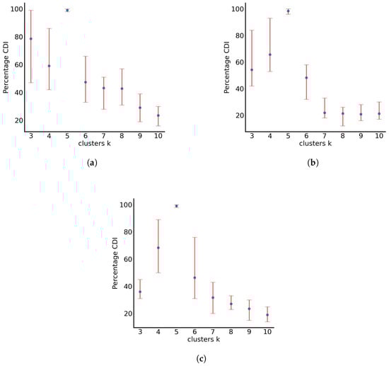
Figure 5.
Percentage averaged CDI for particles with noise standard deviation varying randomly between (a) 0 and 0.1, (b) 0 and 0.5 and (c) 0 and 1.0.
Table 5.
Performance of the RUN-ICON algorithm during particle dispersion when noise standard deviation varies between (a) 0 and 0.1, (b) 0 and 0.5 and (c) 0 and 1.0.
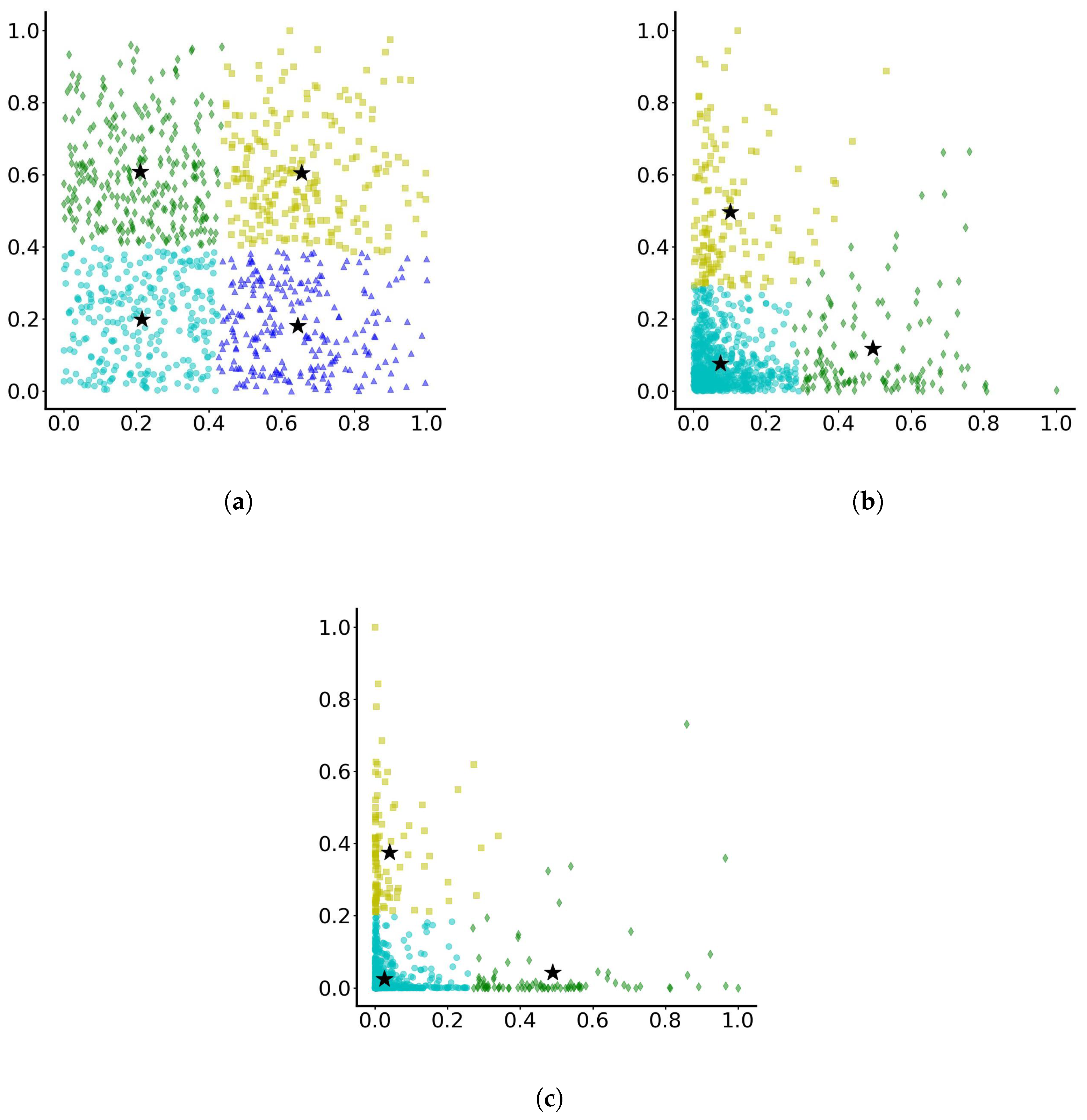
The dominant clustering of particles on normalised axes is presented in Figure 6, where the final positions of particles are shown (i.e., after 10-time units) and the related clusters, based on the RUN-ICON predictions. It is observed that when noise is added, with regards to the origin, some particles have travelled north, some south, some east and some west. At the same time, many of them have remained concentrated around the origin and have not travelled far away from it.

Figure 6.
Dominant clustering of particles with noise standard deviation varying randomly between (a) 0 and 0.1, (b) 0 and 0.5 and (c) 0 and 1.0. The stars indicate the cluster centres. Different colours indicate different clusters.
Once again, the three new clustering experiments were repeated with repeat K-means and Bayesian K-means and their clustering efficiencies using the SC were determined. The results appear in Table 6, Table 7 and Table 8, for the three different test cases, where noise standard deviation varies within the range (0, 0.1), (0, 0.5) and (0, 1.0), respectively.
Table 6.
Clustering efficiency of repeat and Bayesian K-means algorithms when noise standard deviation varies between 0 and 0.1.
Table 7.
Clustering efficiency of repeat and Bayesian K-means algorithms when noise standard deviation varies between 0 and 0.5.
Table 8.
Clustering efficiency of repeat and Bayesian K-means algorithms when noise standard deviation varies between 0 and 1.0.
As shown in Table 6, the repeat K-means algorithm exhibits low SC across all clusters, ranging from 0.3 to 0.4. This indicates that the algorithm struggles to identify a distinct dominant clustering pattern. Interestingly, the separation into five clusters yields the highest SC, albeit relatively low. On the other hand, when employing Bayesian K-means, all SCs are remarkably low, with the lowest value observed for the five-cluster configuration, in contrast to the results obtained with the other two methods. The highest SC is achieved when the data is separated into three clusters, implying a relatively better clustering performance for this configuration than others.
The results in Table 7 indicate that repeat K-means exhibits low SC (ranging from 0.3 to 0.4), suggesting the algorithm’s inability to identify a clear dominant clustering pattern. Interestingly, the separation into five clusters shows marginally higher SC than other configurations. In the case of Bayesian K-means, all SCs are extremely low, implying the algorithm’s limited ability to establish dominant clusters. Notably, the highest SC is observed when the data are partitioned into five clusters, in agreement with the other methods.
Table 8 presents the results for noise standard deviation varying randomly between 0 and 1.0. Once again, repeat K-means shows low SC (all between 0.3 and 0.4), indicating its inability to identify a dominant clustering pattern. The separation into five clusters yields the highest SC, albeit marginally. As for Bayesian K-means, all SCs are predicted to be very low, suggesting the algorithm’s limitations in determining dominant clustering. Surprisingly, the highest SC is observed when the data is divided into six clusters, which differs from the predictions of the other two methods.
Once more, the DBSCAN algorithm was applied to the normalised data of all three test cases with different combinations of and . The algorithm failed again to find more than one cluster for any combination of the two. The hyperparameters of the DBSCAN algorithm, and , as before, took values from the sets (0.1, 0.3, 0.5, 0.7) and (5, 10, 15), respectively.
Particle Dispersion with c’s and d’s in Range (0, 1) and in Range (0, 0.1)
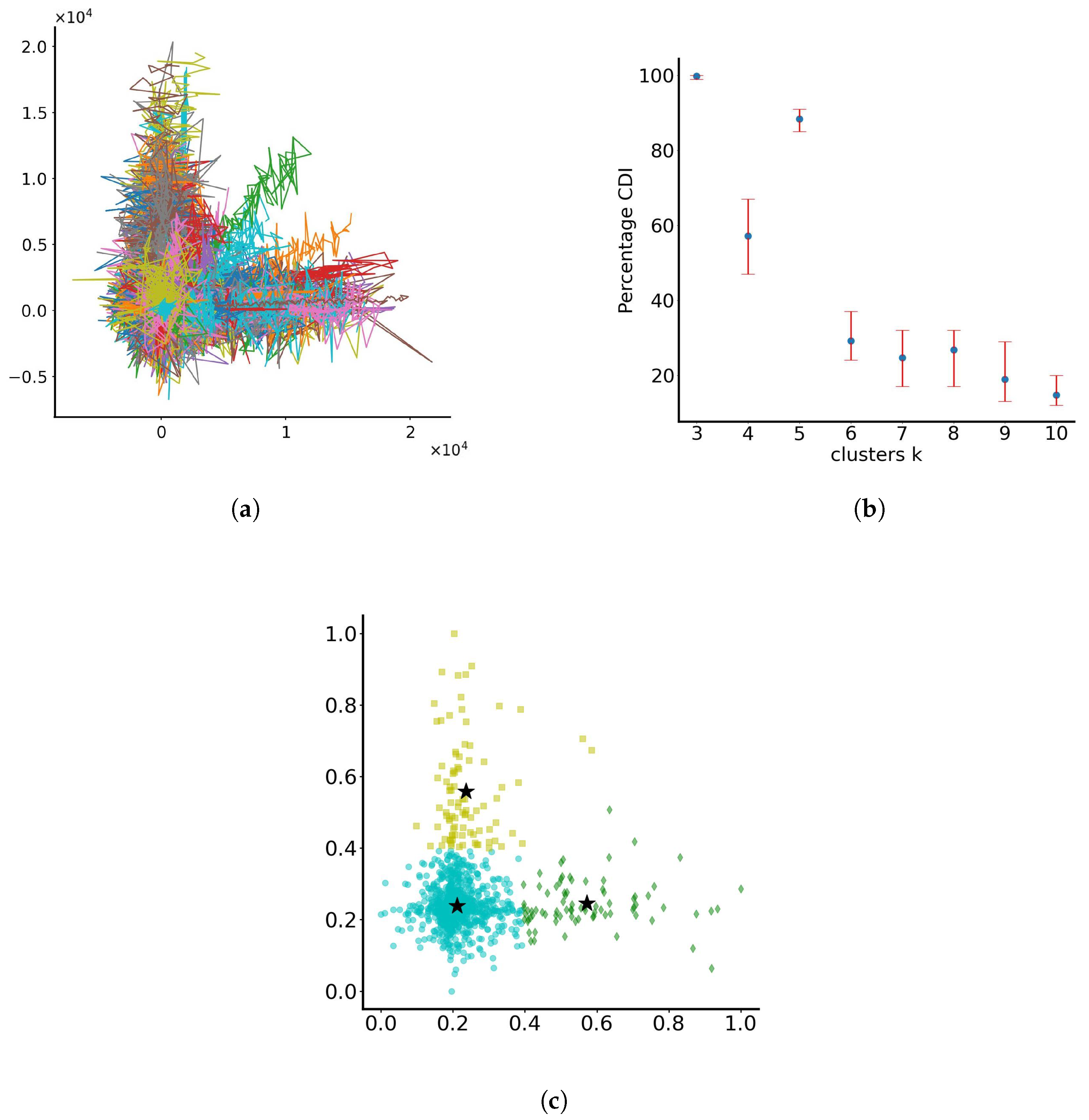
This experiment is treated differently from the rest since the range of values of the is such that the dispersed particles marginally retain their trajectories, as the ones seen in Figure 1c (biased trajectories along positive x and y axes). At the same time, they try to form the same rhomboid-like shape, as seen in Figure 4. The particle trajectories in the dimensionless x-y plane are shown in Figure 7a. When applying the RUN-ICON algorithm to find the optimal clustering, it becomes obvious that separation in three clusters dominates (with average CDI and Uncertainty being 0.998 and 0.01, respectively). The algorithm, at that stage of motion, separates the particles in groups of particles that remain around the origin, particles that have travelled away from the origin mostly in the positive x direction and particles that have travelled away from the origin mostly in the positive y direction. The second best option would be separating into five clusters (as with all rhomboid-like shapes examined in this section). The RUN-ICON clustering results are seen in Figure 7b, while Figure 7c presents the three distinct groups of optimal clustering for the normalised data set.
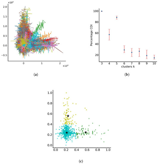
Figure 7.
Clustering of particles with parameters c and d varying randomly in the range (0, 1) and noise standard deviation varying randomly in the range (0, 0.1). (a) Particle trajectories in the dimensionless x-y plane. Each line represents the trajectory of a single particle. The colours assigned to the lines serve the purpose of discretising trajectories for individual particles. (b) RUN-ICON dominant clustering results. (c) Optimal clustering in 3 groups. The stars indicate the cluster centres. Different colours indicate different clusters.
In Table 9, results are presented when repeat and Bayesian K-means algorithms are applied to the normalised data set of the final particle positions. As may be observed, this is the only instance that repeats K-means predicted with relative confidence data separation into three clusters (relatively high SC value and lower for all other clusterings). However, it failed to predict the second-best clustering into five groups (as predicted by RUN-ICON), indicating its inability to identify secondary dominant patterns. As for Bayesian K-means, it predicts separation into four groups (in contrast to the predictions of the other two methods), while all other SC values are predicted to be very low. When DBSCAN was also applied to the data set (with the same combination of hyperparameters), it failed again to separate the data set into more than one cluster.
Table 9.
Clustering efficiency of repeat and Bayesian K-means algorithms when c’s and d’s vary between 0 and 1.0 and noise standard deviation varies between 0 and 0.1.
In conclusion, all algorithms tested so far (namely, repeat K-means, Bayesian K-means and DBSCAN) demonstrate notably inferior results when compared to the performance of RUN-ICON. These algorithms exhibit a lack of capability in discerning dominant clustering patterns effectively. Once again, Bayesian K-means proved extremely time-consuming, as observed and discussed in the previous section.
5. Conclusions
We presented unsupervised learning on 1000 non-interacting particles, released from a singular source and left to propagate in the 2-D plane, based on a set of differential equations, where their parameters were randomly selected from a uniform distribution. Their trajectories and final positions were recorded after 10 dimensionless time units in the dimensionless x-y plane. The particles were clustered using the RUN-ICON algorithm based on their final positions.
The algorithm separated the particles into either four clusters (for the smallest range of parameters c and d) or three clusters (for the higher ranges of parameters c and d, when particle separation was evident) with high confidence and low uncertainty. In contrast, the repeat and Bayesian K-means and DBSCAN algorithms did not manage to separate the particles confidently. Moreover, when noise was added to the system, RUN-ICON predicted with increased confidence (almost 100%) the separation of the particles in five clusters (or three, in the case of c’s and d’s varying randomly within the range (0, 1) and within the range (0, 0.1)). The performance of the other methods was unsatisfactory. These findings provide evidence about the accuracy and efficiency of the RUN-ICON algorithm, which performs extremely well in data sets where noise is present.
We will utilise the algorithm in diverse applications involving the dispersion of particles with time, where experimental and numerical data are available. Applying UL to particle dispersion will enhance our understanding of particle dynamics and their impact on air quality, health and climate.
Author Contributions
Conceptualization, N.C. and D.D.; methodology, N.C. and D.D.; formal analysis, N.C. and D.D.; investigation, N.C. and D.D.; resources, D.D.; writing, N.C. and D.D.; project administration, D.D.; funding acquisition, D.D.; contribution to the discussion N.C. and D.D. All authors have read and agreed to the published version of the manuscript.
Funding
This paper is supported by the European Union’s Horizon Europe Research and Innovation Actions programme under grant agreement No. 101069937, project name: HS4U (HEALTHY SHIP 4U). Views and opinions expressed are those of the author(s) only and do not necessarily reflect those of the European Union or the European Climate, Infrastructure, and Environment Executive Agency. Neither the European Union nor the granting authority can be held responsible for them.
Data Availability Statement
Not applicable.
Conflicts of Interest
The authors declare no conflict of interest.
References
- Hinton, G.E.; Dayan, P.; Frey, B.J.; Neal, R.M. The “Wake-Sleep” Algorithm for Unsupervised Neural Networks. Science 1995, 268, 1158–1161. [Google Scholar] [CrossRef] [PubMed]
- Krotov, D.; Hopfield, J.J. Unsupervised learning by competing hidden units. Proc. Natl. Acad. Sci. USA 2019, 116, 7723–7731. [Google Scholar] [CrossRef] [PubMed]
- Hadsell, R.; Chopra, S.; LeCun, Y. Dimensionality reduction by learning an invariant mapping. In Proceedings of the 2006 IEEE Computer Society Conference on Computer Vision and Pattern Recognition (CVPR’06), New York, NY, USA, 17–22 June 2006; Volume 2, pp. 1735–1742. [Google Scholar]
- Dbouk, T.; Drikakis, D. On respiratory droplets and face masks. Phys. Fluids 2020, 32, 063303. [Google Scholar] [CrossRef] [PubMed]
- Dbouk, T.; Drikakis, D. Weather impact on airborne coronavirus survival. Phys. Fluids 2020, 32, 093312. [Google Scholar] [CrossRef] [PubMed]
- Dbouk, T.; Drikakis, D. Fluid Dynamics and Epidemiology: Seasonality and Transmission Dynamics. Phys. Fluids 2021, 33, 021901. [Google Scholar] [CrossRef]
- Van Rijn, C.; Somsen, G.A.; Hofstra, L.; Dahhan, G.; Bem, R.A.; Kooij, S.; Bonn, D. Reducing aerosol transmission of SARS-CoV-2 in hospital elevators. Indoor Air 2020, 30, 1065–1066. [Google Scholar] [CrossRef]
- Satheesan, M.K.; Mui, K.W.; Wong, L.T. A numerical study of ventilation strategies for infection risk mitigation in general inpatient wards. Build. Simul. 2020, 13, 887–896. [Google Scholar] [CrossRef]
- Katramiz, E.; Al Assaad, D.; Ghaddar, N.; Ghali, K. The effect of human breathing on the effectiveness of intermittent personalized ventilation coupled with mixing ventilation. Build. Environ. 2020, 174, 106755. [Google Scholar] [CrossRef]
- Katramiz, E.; Ghaddar, N.; Ghali, K.; Al-Assaad, D.; Ghani, S. Effect of individually controlled personalized ventilation on cross-contamination due to respiratory activities. Build. Environ. 2021, 194, 107719. [Google Scholar] [CrossRef]
- Shao, S.; Zhou, D.; He, R.; Li, J.; Zou, S.; Mallery, K.; Kumar, S.; Yang, S.; Hong, J. Risk assessment of airborne transmission of COVID-19 by asymptomatic individuals under different practical settings. J. Aerosol Sci. 2020, 151, 105661. [Google Scholar] [CrossRef]
- Hu, M.; Lin, H.; Wang, J.; Xu, C.; Tatem, A.J.; Meng, B.; Zhang, X.; Liu, Y.; Wang, P.; Wu, G.; et al. Risk of Coronavirus Disease 2019 Transmission in Train Passengers: An Epidemiological and Modeling Study. Clin. Infect. Dis. 2020, 72, 604–610. [Google Scholar] [CrossRef] [PubMed]
- Abuhegazy, M.; Talaat, K.; Anderoglu, O.; Poroseva, S.V. Numerical investigation of aerosol transport in a classroom with relevance to COVID-19. Phys. Fluids 2020, 32, 103311. [Google Scholar] [CrossRef] [PubMed]
- Rowe, B.; Canosa, A.; Drouffe, J.; Mitchell, J. Simple quantitative assessment of the outdoor versus indoor airborne transmission of viruses and COVID-19. Environ. Res. 2021, 198, 111189. [Google Scholar] [CrossRef] [PubMed]
- Golkarfard, V.; Talebizadeh, P. Numerical comparison of airborne particles deposition and dispersion in radiator and floor heating systems. Adv. Powder Technol. 2014, 25, 389–397. [Google Scholar] [CrossRef]
- Mao, S.; Lang, J.; Chen, T.; Cheng, S. Improving source inversion performance of airborne pollutant emissions by modifying atmospheric dispersion scheme through sensitivity analysis combined with optimization model. Environ. Pollut. 2021, 284, 117186. [Google Scholar] [CrossRef]
- Pantusheva, M.; Mitkov, R.; Hristov, P.O.; Petrova-Antonova, D. Air Pollution Dispersion Modelling in Urban Environment Using CFD: A Systematic Review. Atmosphere 2022, 13, 1640. [Google Scholar] [CrossRef]
- Fernández-Pacheco, V.M.; Álvarez Álvarez, E.; Blanco-Marigorta, E.; Ackermann, T. CFD model to study PM10 dispersion in large-scale open spaces. Sci. Rep. 2023, 13, 5966. [Google Scholar] [CrossRef]
- Mei, S.J.; Luo, Z.; Zhao, F.Y.; Wang, H.Q. Street canyon ventilation and airborne pollutant dispersion: 2-D versus 3-D CFD simulations. Sustain. Cities Soc. 2019, 50, 101700. [Google Scholar] [CrossRef]
- Yan, X.; Li, T.; Hu, C.; Wu, Q. Real-time localization of pollution source for urban water supply network in emergencies. Clust. Comput. 2019, 22, 5941–5954. [Google Scholar] [CrossRef]
- Geng, G.; Xiao, Q.; Liu, S.; Liu, X.; Cheng, J.; Zheng, Y.; Xue, T.; Tong, D.; Zheng, B.; Peng, Y.; et al. Tracking air pollution in China: Near real-time PM2.5 retrievals from multisource data fusion. Environ. Sci. Technol. 2021, 55, 12106–12115. [Google Scholar] [CrossRef]
- Drewil, G.I.; Al-Bahadili, R.J. Forecast air pollution in smart city using deep learning techniques: A review. Multicult. Educ. 2021, 7, 38–47. [Google Scholar]
- Hulkkonen, M.; Lipponen, A.; Mielonen, T.; Kokkola, H.; Prisle, N.L. Changes in urban air pollution after a shift in anthropogenic activity analysed with ensemble learning, competitive learning and unsupervised clustering. Atmos. Pollut. Res. 2022, 13, 101393. [Google Scholar] [CrossRef]
- Kokkinakis, I.W.; Drikakis, D. Nuclear explosion impact on humans indoors. Phys. Fluids 2023, 35, 016114. [Google Scholar] [CrossRef]
- Kassandros, T.; Bagkis, E.; Johansson, L.; Kontos, Y.; Katsifarakis, K.L.; Karppinen, A.; Karatzas, K. Machine learning-assisted dispersion modelling based on genetic algorithm-driven ensembles: An application for road dust in Helsinki. Atmos. Environ. 2023, 307, 119818. [Google Scholar] [CrossRef]
- Rybarczyk, Y.; Zalakeviciute, R. Machine Learning Approaches for Outdoor Air Quality Modelling: A Systematic Review. Appl. Sci. 2018, 8, 2570. [Google Scholar] [CrossRef]
- Madan, T.; Sagar, S.; Virmani, D. Air quality prediction using machine learning algorithms—A review. In Proceedings of the 2020 2nd International Conference on Advances in Computing, Communication Control and Networking (ICACCCN), Greater Noida, India, 18–19 December 2020; pp. 140–145. [Google Scholar]
- Lee, J.; Lee, G. Feature Alignment by Uncertainty and Self-Training for Source-Free Unsupervised Domain Adaptation. Neural Netw. 2023, 161, 682–692. [Google Scholar] [CrossRef]
- Lee, J.; Lee, G. Unsupervised domain adaptation based on the predictive uncertainty of models. Neurocomputing 2023, 520, 183–193. [Google Scholar] [CrossRef]
- Mousavi, Z.; Yousefi Rezaii, T.; Sheykhivand, S.; Farzamnia, A.; Razavi, S. Deep convolutional neural network for classification of sleep stages from single-channel EEG signals. J. Neurosci. Methods 2019, 324, 108312. [Google Scholar] [CrossRef]
- Mousavi, Z.; Varahram, S.; Mohammad Ettefagh, M.; Sadeghi, M.H. Dictionary learning-based damage detection under varying environmental conditions using only vibration responses of numerical model and real intact State: Verification on an experimental offshore jacket model. Mech. Syst. Signal Process. 2023, 182, 109567. [Google Scholar] [CrossRef]
- Lloyd, S. Least squares quantization in PCM. IEEE Trans. Inf. Theory 1982, 28, 129–137. [Google Scholar] [CrossRef]
- Everitt, B.S.; Landau, S.; Leese, M.; Stahl, D. Hierarchical Clustering. In Cluster Analysis; John Wiley & Sons, Ltd.: Hoboken, NJ, USA, 2011; Chapter 4; pp. 71–110. [Google Scholar] [CrossRef]
- Ester, M.; Kriegel, H.P.; Sander, J.; Xu, X. A density-based algorithm for discovering clusters in large spatial databases with noise. In Proceedings of the Kdd, Portland, OR, USA, 2–4 August 1996; Volume 96, pp. 226–231. [Google Scholar]
- Hinton, G.E.; Salakhutdinov, R.R. Reducing the Dimensionality of Data with Neural Networks. Science 2006, 313, 504–507. [Google Scholar] [CrossRef] [PubMed]
- Kingma, D.P.; Welling, M. An Introduction to Variational Autoencoders. Found. Trends® Mach. Learn. 2019, 12, 307–392. [Google Scholar] [CrossRef]
- Schneider, R.; Vicedo-Cabrera, A.M.; Sera, F.; Masselot, P.; Stafoggia, M.; de Hoogh, K.; Kloog, I.; Reis, S.; Vieno, M.; Gasparrini, A. A satellite-based spatio-temporal machine learning model to reconstruct daily PM2.5 concentrations across Great Britain. Remote Sens. 2020, 12, 3803. [Google Scholar] [CrossRef]
- Fillola, E.; Santos-Rodriguez, R.; Manning, A.; O’Doherty, S.; Rigby, M. A machine learning emulator for Lagrangian particle dispersion model footprints: A case study using NAME. Geosci. Model Dev. 2023, 16, 1997–2009. [Google Scholar] [CrossRef]
- Stubbemann, M.; Hille, T.; Hanika, T. Selecting Features by their Resilience to the Curse of Dimensionality. arXiv 2023, arXiv:2304.02455. [Google Scholar]
- Christakis, N.; Drikakis, D. Reducing Uncertainty and Increasing Confidence in Unsupervised Learning. Mathematics 2023, 11, 3063. [Google Scholar] [CrossRef]
- Fränti, P.; Sieranoja, S. How much can k-means be improved by using better initialization and repeats? Pattern Recognit. 2019, 93, 95–112. [Google Scholar] [CrossRef]
- Kulis, B.; Jordan, M.I. Revisiting K-Means: New Algorithms via Bayesian Nonparametrics. In Proceedings of the 29th International Coference on International Conference on Machine Learning, Omnipress, ICML’12, Madison, WI, USA, 26 June–1 July 2012; pp. 1131–1138. [Google Scholar]
- Dhand, R.; Li, J. Coughs and Sneezes: Their Role in Transmission of Respiratory Viral Infections, Including SARS-CoV-2. Am. J. Respir. Crit. Care Med. 2020, 202, 651–659. [Google Scholar] [CrossRef]
- Shutaywi, M.; Kachouie, N. Silhouette Analysis for Performance Evaluation in Machine Learning with Applications to Clustering. Entropy 2021, 23, 759. [Google Scholar] [CrossRef]
- Wade, S. Bayesian cluster analysis. Philos. Trans. Ser. A Math. Phys. Eng. Sci. 2023, 381, 20220149. [Google Scholar] [CrossRef]

Disclaimer/Publisher’s Note: The statements, opinions and data contained in all publications are solely those of the individual author(s) and contributor(s) and not of MDPI and/or the editor(s). MDPI and/or the editor(s) disclaim responsibility for any injury to people or property resulting from any ideas, methods, instructions or products referred to in the content. |
© 2023 by the authors. Licensee MDPI, Basel, Switzerland. This article is an open access article distributed under the terms and conditions of the Creative Commons Attribution (CC BY) license (https://creativecommons.org/licenses/by/4.0/).