Article

Multivariate Bayesian Semiparametric Regression Model for Forecasting and Mapping HIV and TB Risks in West Java, Indonesia

1
Center of Epidemiology, Department of Statistics, Universitas Padjadjaran, Jl. Raya Bandung Sumedang km 21 Jatinangor, Sumedang 45363, Indonesia
2
Center of Flexible Modeling, Department of Statistics, Universitas Padjadjaran, Jl. Raya Bandung Sumedang km 21 Jatinangor, Sumedang 45363, Indonesia
3
Department of Mathematics, Parahyangan University, Jl. Ciumbuleuit No. 94, Hegarmanah, Kec. Cidadap, Kota Bandung 40141, Indonesia
*
Author to whom correspondence should be addressed.
Mathematics 2023, 11(17), 3641; https://doi.org/10.3390/math11173641
Submission received: 22 July 2023 / Revised: 17 August 2023 / Accepted: 21 August 2023 / Published: 23 August 2023
(This article belongs to the Section Mathematical Biology)

Abstract

:
Multivariate “Bayesian” regression via a shared component model has gained popularity in recent years, particularly in modeling and mapping the risks associated with multiple diseases. This method integrates joint outcomes, fixed effects of covariates, and random effects involving spatial and temporal components and their interactions. A shared spatial–temporal component considers correlations between the joint outcomes. Notably, due to spatial–temporal variations, certain covariates may exhibit nonlinear effects, necessitating the use of semiparametric regression models. Sometimes, choropleth maps based on regional data that is aggregated by administrative regions do not adequately depict infectious disease transmission. To counteract this, we combine the area-to-point geostatistical model with inverse distance weighted (IDW) interpolation for high-resolution mapping based on areal data. Additionally, to develop an effective and efficient early warning system for controlling disease transmission, it is crucial to forecast disease risk for a future time. Our study focuses on developing a novel multivariate Bayesian semiparametric regression model for forecasting and mapping HIV and TB risk in West Java, Indonesia, at fine-scale resolution. This novel approach combines multivariate Bayesian semiparametric regression with geostatistical interpolation, utilizing population density and the Human Development Index (HDI) as risk factors. According to an examination of annual data from 2017 to 2021, HIV and TB consistently exhibit recognizable spatial patterns, validating the suitability of multivariate modeling. The multivariate Bayesian semiparametric model indicates significant linear effects of higher population density on elevating HIV and TB risks, whereas the impact of the HDI varies over time and space. Mapping of HIV and TB risks in 2022 using isopleth maps shows a clear HIV and TB transmission pattern in West Java, Indonesia.

1. Introduction

Spatiotemporal disease mapping is a common modeling technique used to understand the geographical evolution of disease risks as well as generate hypotheses regarding critical risk factors [1,2,3,4,5]. It typically involves geographically visualizing disease risks in small areas over time [2]. Typically, spatiotemporal disease-mapping models are presented as generalized additive mixed model (GAMM) within a full Bayesian framework [6]. The model includes the fixed effects of the covariates as well as spatial and temporal random effects and the spatiotemporal interaction [7]. The principal focuses of disease-mapping models are disease map reconstruction, model evaluation, and the quantification of multiple risk factors for spatiotemporal variation in disease risk [8,9].
Spatiotemporal disease mapping is commonly approached through univariate modeling, which focuses on a single disease. However, progress has been made to incorporate additional analysis techniques such as joint spatiotemporal modeling for several related diseases with shared etiological risk factors [10,11,12,13,14]. Borrowing information across diseases helps identify patterns and conditions one disease on others, which is valuable when dealing with sparse disease counts or underreporting [15]. This improvement allows the identification of shared and divergent trends, thereby improving disease risk prediction accuracy [16,17]. The shared component model is a frequently employed approach for conducting multivariate spatiotemporal disease modeling. The model differentiates the underlying risk for each disease while identifying shared risk factors for multiple diseases [17,18]. However, incorporating multiple diseases into spatiotemporal modeling approaches for forecasting disease risk simultaneously introduces significant model complexity, primarily due to the massive number of parameters that must be estimated [19]. The full Bayesian approach offers an appropriate framework for addressing these complexities through the hierarchical structure [20,21,22]. One of the unique advantages of the Bayesian method is its robustness in interpreting the posterior distribution and making inferences for parameters of interest [23,24]. Hence, there has been a significant rise in the adoption of multivariate spatiotemporal approaches that utilize comprehensive Bayesian shared component models to simultaneously model multiple diseases [5,20,25].
In spatiotemporal disease modeling, it is common to include multiple covariates to identify significant risk factors. It is frequently assumed that these covariates demonstrate linear effects over both space and time. Nonetheless, due to the existence of spatiotemporal heterogeneity, specific covariates might display nonlinear effects or exhibit variations across space and time [26]. To accommodate both linear and nonlinear effects of the covariates, semiparametric regression models were developed [26,27]. The main advantage of the semiparametric regression model lies in its superior prediction accuracy [28]. Additionally, to establish a robust and proficient early warning system (EWS), it is crucial to construct a model capable of not only predicting disease occurrences at past and present time points but also forecasting disease risks in the future, particularly with high-resolution maps on a fine spatiotemporal scale [29,30]. Based on the available information, the author is not aware of any publications that explore the multivariate semiparametric regression model for forecasting and mapping risk at fine-scale resolution. High-resolution maps can offer detailed information on high-risk zones and the localized nature of disease transmission at fine-scale resolution, particularly in identifying the causes and transmission mechanisms of diseases [31,32].
To generate high-resolution maps that effectively depict the intricate patterns of disease transmission at a fine-scale resolution, it is imperative to formulate a regression model incorporating suitable predictors that are accessible at high-level resolution. Within this model, the values attributed to areal entities function as linear constraints [32,33,34]. Nonetheless, the process of gathering predictors for high-resolution purposes encountered challenges. Consequently, alternative high-resolution maps are generated primarily through interpolation techniques that rely on a distance function, Tobler’s first fundamental law of geography [35,36,37]. This law states that everything is interconnected, but objects in proximity have stronger relationships than those at a distance [38]. In addition, spatial interpolation emphasizes that values to be evaluated at a particular point are primarily influenced by nearby points as opposed to those further away. High-resolution maps generated from areal data are developed using the area-to-point geostatistical model [36,37,39]. This geostatistical model employs disaggregation techniques to generate detailed and comprehensive isopleth maps, utilizing variable data of interest at a lower-resolution. For geospatial interpolation, models include inverse distance weighted (IDW) or model-based approaches such as Kriging and the Gaussian process (GP) [35,40]. IDW stands as a popular interpolation method in disease-mapping studies [35]. Based on areal data, Ref. [41] utilized IDW to create high-resolution maps for dengue disease transmission, and Ref. [35] used IDW to develop high-resolution maps for COVID-19 disease. Unlike model-based interpolation methods, IDW interpolation is a precise technique that estimates a point’s value by considering its proximity to nearby known points rather than distant points. IDW interpolates by calculating values for uncertain regions based on the expected trends of neighboring regions, adhering to Tobler’s first law of geography [35,36,37]. IDW operates according to the principle of inverse distances; weightage increases as distance decreases and vice versa. This implies that the values of known data points approximate those of unknown ones. IDW requires known point values, unlike other methods such as isopleth mapping, which utilizes assigned points such as polygon centroids [35]. As per references [35,36,37], despite the area data interpolation relying on polygon centroids, the simulation outcomes demonstrate that this interpolation method yields precise prediction results. This approach demands less computational effort to satisfy statistical assumptions. However, according to [40], IDW exhibits a similar goodness-of-fit performance when compared to GP.
Forecasting disease risk at fine-scale resolution facilitates the targeting of future intervention programs, allowing for more effective and efficient EWS programs [31]. Forecasting and mapping are constructed using a two-step approach. Firstly, accurate forecasts are obtained through multivariate Bayesian semiparametric regression models. Multivariate semiparametric regression models are basically generalized additive mixed models (GAMM). The model includes fixed and random effects additively with multiple responses [42]. Secondly, high-resolution maps are constructed by employing IDW interpolation techniques on the forecasted values.
Our study aims to develop a multivariate Bayesian semiparametric regression model for forecasting and mapping of HIV and TB risks in West Java, Indonesia at a fine-scale resolution. These communicable diseases are notably influenced by population mobility, particularly in neighboring regions with prevalent social interactions. The foundation of an early warning system for HIV and TB hinges on spatiotemporal high-resolution maps. However, the available data for HIV and TB are presented in aggregated format and reported according to administrative areas due to privacy, administrative, technical, or other considerations. To address this challenge, the area-to-point model becomes indispensable. This disaggregation model facilitates the creation of continuous and detailed isopleth maps. Population density and the Human Development Index (HDI) are hypothesized to explain the spatiotemporal variations of HIV and TB in West Java Province. The assertion is supported by the results of previous research [43,44,45,46]. We consider the effects of population density to be linear or constant across space and time and the HDI to be non-linear or vary across space and time. The remainder of this paper has the following structure. The multivariate Bayesian semiparametric regression model for forecasting and high-resolution mapping is introduced in Section 2. The third section applies the methodology to the HIV and TB risks in West Java, Indonesia. A discussion and the conclusions are presented in Section 4 and Section 5, respectively.

2. Multivariate Bayesian Semiparametric Regression Model for Forecasting and High-Resolution Mapping

2.1. Generalized Additive Mixed Model via Log Linear Model

Because the HIV and TB data are count datasets, we employed the GAMM through a log-linear model while assuming the data followed Poisson or negative binomial (NB) distributions [41]. Specifically, for each area ( i ) and year ( t ), we modeled the number of reported cases ( y d i t ) for disease ( d ), where ( d = 1 ) represents HIV; ( d = 2 ) represents TB; i = 1 , , n with t = 1 , , T ; n represents the number of nonoverlapping areas; T is the total time points. Let us first assume the number of reported cases y d i t follows a Poisson distribution with a mean of E y d i t = λ d i t and a corresponding variance of V a r y d i t = λ d i t [47]:
y d i t | λ d i t ~ P o i s s o n λ d i t ,   d = 1 , 2 ,   i = 1 , , n ,   and   t = 1 , , T
with the probability mass function as:
p y d i t | λ d i t = e λ d i t λ d i t y d i t y d i t !   for   y d i t = 0 , 1 , 2 ,
where the mean λ d i t = E d i t θ d i t with E d i t denotes the expected number of reported cases and θ d i t the relative risk for disease d at location i and time t. The computation of E d i t was conducted for each disease, area, and year as follows [41]:
E d i t = N i t × p d ; for   d = 1 , 2 ,   i = 1 , , n ,   and   t = 1 , , T
where N i t denotes the population at risk at area i and time t, and p d denotes the probability of disease d occurring across all regions within T time periods. For d = 1 , 2 , the p d is defined as follows [41]:
p d = i = 1 n t = 1 T y d i t i = 1 n t = 1 T N i t    
Overdispersion is a critical issue in count data modeling. It refers to the condition in which the variance in the number of cases is much greater than its mean V a r y i t > E y i t . Overdispersion is caused by many factors, including excess zero and heterogeneity issues [41]. One way to address this issue is by introducing a second parameter, ϵ d i t , into the Poisson distribution. This parameter is assumed to follow a Gamma distribution, where each distribution for d = 1   and d = 2   has an equal scale and shape parameter (denoted as d ) [48]:
p d = i = 1 n t = 1 T y d i t i = 1 n t = 1 T N i t    
The parameter d also accounts for the overdispersion parameter. The combination of Poisson and Gamma distributions produces the Poisson–Gamma distribution with the probability distribution function as [48]:
p y d i t | E d i t , θ d i t , ϵ d i t = Gamma d , d Poisson E d i t θ d i t = d d ϵ d i t d 1 exp d ϵ d i t Γ ϵ d i t exp E d i t θ d i t E d i t θ d i t y d i t y d i t ! .
The NB distribution is obtained by integrating out the second parameter ϵ d i t from Equation (6) with the probability distribution expressed as [48]:
p y d i t | E d i t , θ d i t , d = Γ y d i t + d Γ y d i t + 1 Γ d E d i t θ d i t E d i t θ d i t + d y d i t d E d i t θ d i t + d d .
The mean and variance of NB distribution for disease d at area i and time t are E y d i t = E d i t θ d i t and Var y d i t = E d i t θ d i t + E d i t θ d i t 2 / d , respectively.
Commonly, the risk of diseases is measured using crude rates as an unbiased estimate of the relative risk [49]. It is known as the standardized incidence ratio (SIR). However, this measurement is not reliable, particularly in situations with high population variability and small numbers of disease cases, due to the presence of significant sampling errors. The SIR is calculated by dividing the number of reported cases, y d i t , by the expected number of disease cases, E d i t [47,49]:
S I R d i t = y d i t E d i t   for   d = 1 , 2 ,   i = 1 , , n   and   t = 1 , , T
In addition, using Equation (8), it is not possible to explicitly account for fixed and random effect components. Conversely, the linear predictor of the parameter of the relative risk can be expressed as the log-linear model η d i t = log θ d i t . The log-linear model permits more accurate modeling of the relationship between fixed and random effect components on response variables. The log relative risk ( θ d i t ) for HIV and TB, respectively, can be represented as semiparametric regression models as follows:
η 1 i t = α 1 + β 11 x i t 1 + f 1 i β 12 i x i t 2 + f 1 t β 13 t x i t 2 + δ ω i η 2 i t = α 2 + β 21 x i t 1 + f 2 i β 22 i x i t 2 + f 2 t β 23 t x i t 2 + ω i δ
The linear predictor in our model had several components. These encompassed the overall intercept α 1 and α 2 for HIV and TB, which represented the baseline risk each disease. We also considered the fixed effects β 11 and β 21 , representing the linear effects of population density x i t 1 on HIV and TB, respectively. We incorporated spatiotemporally nonlinear effects of the Human Development Index (HDI) ( x i t 2 ) on HIV and TB as the additive time- and space-varying effects. The space-varying effects were denoted as the smooth or nonlinear functions f 1 s β 12 i x i t 2   and   f 2 s β 22 i x i t 2 , and the time-varying effects were denoted as f 1 t β 13 t x i t 2 and f 2 t β 23 t x i t 2 . The regression parameters β 12 i and β 22 i are space coefficients that accounted for the spatial variation in the relationship between the HDI and the risk of HIV and TB, respectively. Meanwhile, the regression parameters β 13 t and β 23 t are time coefficients that pertained to addressing the temporal variation in the relationship between the HDI and the risk of HIV and TB. The space- and time-varying effects were modeled through random effects components [32,33]. Furthermore, the model incorporated a shared spatial effect ( ω = ω i for i = 1 , , n ), which captured the spatial dependence for HIV and TB. The scale parameter δ determined the magnitude of this shared spatial effect.
The multivariate semiparametric model in Equation (9) can be written as a simple model:
  η d i t = α d + β d 1 x i t 1 + f d t β d 2 i x i t 2 + f d t β d 3 t x i t 2 + δ d ω i
where for d = 1 ,   δ d = δ ; and for d = 2 , δ d = 1 / δ .

2.2. Bayesian Specification

We used a Bayesian approach via Latent Gaussian Modeling (LGM) to estimate the multivariate semiparametric regression model in Equation (10). The Bayesian LGM approach integrates the likelihood function and the Gaussian prior distribution, leading to the derivation of the Gaussian posterior distribution [50]. Subsequently, the posterior distribution was employed to estimate the parameters of interest [4]. The Bayesian approach provides a robust framework for modeling complex structures, especially accommodating nonlinear modeling in scenarios with discrete responses. LGM facilitates the implementation of models, including Poisson and NB regression models [41]. According to the above discussion, we applied Poisson and NB distributions as the likelihood functions. For α d and   β d 1 , we assigned a vague Gaussian prior characterized by a zero mean and a large variance; those are α d , β d 1 ~ N 0 , 10 6 . A Gaussian distribution with a large variance ensures that the random variable can encompass a wide range of possible values. We assigned a Leroux Conditional Autoregressive (LCAR) prior for spatially varying effects on β d 3 i . This prior distribution considered the spatial relationship between adjacent regions. We used a neighborhood matrix W based on contiguity to define this relationship, where areas that shared a border were considered neighbors. The LCAR spatial prior ensures a certain level of correlation between geographically contiguous regions. The LCAR priors for β d 2 i for d = 1 , 2 were defined as a Gaussian distribution [51]:
β d 2 i | β d 2 , i , σ β d 2 2 , W ~ N τ d j = 1 n w i j β d 2 j τ d j = 1 n w i j + 1 τ d , σ β d 2 2 τ d j = 1 n w i j + 1 τ d
where   every   t   , d = 1 , 2   and   i = 1 , , n . τ d is the spatial correlation coefficient of the HDI on HIV ( d = 1 ) and TB ( d = 2 ), and σ β d 2 2 is the variance that controls for the variability in β d 2 = β d 21 , , β d 2 n . To make sure that τ d remained within the interval of 0 to 1, we assigned a Gaussian prior for log τ d / 1 τ d ~ N 0 , 0.45 [52]. We assigned a random walk of order one (RW1) for temporally varying effects of the HDI. RW1 was defined as a random step at each point in time Δ β d 3 , t = β d 3 , t β d 3 , t 1 . All random steps followed a Gaussian distribution characterized by zero mean and variance σ β d 3 2 [4]:
β d 3 , t , β d 3 , t 1 | σ β d 3 2 ~ N 0 , σ β d 3 2  
where σ β d 3 2 is the variance hyperparameter of β d 3 = β d 31 , , β d 3 T . We assumed spatially shared effect ω i followed LCAR, which is defined as follows:
ω i | ω i , σ ω 2 , W ~ N ρ j = 1 n w i j ω j ρ j = 1 n w i j + 1 ρ , σ ω 2 ρ j = 1 n w i j + 1 ρ     t   and     i = 1 , , n
where ρ is the spatial correlation coefficient of the spatially share component, and σ ω 2 is the variance that controls for the variability of the spatially shared component ω = ω 1 , , ω n . A Gaussian prior distribution was also assigned for log ρ / 1 ρ ~ N 0 , 0.45 [52]. We employed log δ following a vague Gaussian distribution characterized by a zero mean and large variance; that is, log δ ~ N 0 , 10 6 . We assigned the half-Cauchy prior distribution for the standard deviation hyperparameters σ β 12 , σ β 22 , σ β 13 , σ β 23 , and σ ω with its zero-truncated characteristics. The half-Cauchy density function is defined as [53]:
p σ j | γ = 2 π γ 1 + σ j / γ 2   for   σ j = σ β 12 , σ β 22 , σ β 13 , σ β 23 , σ ω
where γ denotes the scale parameter. Following [53], we defined the scale parameter γ = 25 .
Utilizing a Bayesian approach offers a significant benefit, as it enables the computation of the exceedance probability for the relative risk estimate ( θ ^ d i t ) . This is particularly useful in identifying and informing the hot-spot areas of HIV and TB diseases [20]. It is formulated as:
Pr θ ^ d i t > c | y = 1 θ ^ d i t c p θ ^ d i t | y d θ ^ d i t
where c denotes a threshold for the relative and usually defines c = 1 . If the Pr θ ^ d i t > c | y > 0.95 the areas will be defined as hot spot [32,41].

2.3. Model Fitting Using INLA

The estimation of parameters and hyperparameters for the multivariate semiparametric spatiotemporal model in Equation (10) was conducted using Integrated Nested Laplace Approximation (INLA). Let Φ = α 1 , α 2 , β 11 , β 21 , β 12 , β 22 , β 13 , β 23 , ω , δ denote the latent Gaussian field, and ψ = σ ω 2 , σ β 12 2 , σ β 22 2 , σ β 13 2 , σ β 23 2 is a vector of the hyperparameter. The elements of Φ are conditionally independent with a sparse precision matrix Q i j = 0 for i j with the conditional density function [4,33]:
p Φ | ψ = 2 π 2 n T / 2 Q 1 / 2 exp Φ Q Φ
INLA consists of a three-stage modeling approach as follows [54]:
Stage 1—Data model: y | Φ ~ p y | Φ , ψ :
~ d = 1 2 t = 1 T i = 1 n p y d i t | Φ , ψ
Stage 2—Process model: Φ | ψ ~ p Φ | ψ :
        ~ N 0 , Q ψ 1
Stage 3—Parameter model: ψ ~ p ψ .
Given the data likelihood y, the joint posterior distribution of Φ and ψ is:
p Φ , ψ | y = p Φ , ψ , y p y = p y | Φ , ψ p Φ | ψ p ψ Φ ψ p y | Φ , ψ p Φ | ψ p ψ d Φ d ψ
Due to the marginal likelihood p y = Φ ψ p y | Φ , ψ p Φ | ψ p ψ d Φ d ψ , which does not involve the parameters and hyperparameters of interest, the joint posterior distribution can be expressed simply as [54]:
p Φ , ψ | y p y | Φ , ψ p Φ | ψ p ψ
where “ ” is called “proportional to”. To estimate the parameters and hyperparameters of interest, INLA uses the marginal posterior distribution. It can be explained as follows [54]:
(i)
First, obtain the approximation of the marginal posterior distribution of the hyperparameter:
p ˜ ψ | y = p Φ , ψ | y p Φ | ψ , y p y | Φ , ψ p Φ | ψ p ψ p ˜ Φ | ψ , y Φ = Φ * ψ
where p ˜ Φ | ψ , y is a Gaussian approximation of p Φ | ψ , y that is provided by the Laplace method, and Φ * ψ represents the mode for the given ψ . After p ˜ ψ | y is approximated, the k -th element of the joint hyperparameter ψ is obtained by solving the integration below [33]:
p ˜ ψ k | , y = p ψ | y d ψ k
(ii)
Second, approximate the conditional posterior of the l-th (for l = 1 , , n T ) parameter of interest p Φ l | ψ , y that is needed for calculating the marginal posterior of the parameter of interest. The simplified Laplace approximation of p Φ l | ψ , y on Taylor’s series expansion is defined as [33]:
p ˜ Φ l | ψ , y p Φ , ψ | y p ˜ Φ l | Φ k , ψ , y Φ l = Φ l * Φ l , ψ
where p ˜ Φ l | Φ l , ψ , y is the Laplace–Gaussian approximation to p Φ l | Φ k , ψ , y with Φ l * Φ l , ψ as its mode. Given (i) and (ii), the marginal posterior of the parameter of interest is defined as:
p ˜ Φ l | y p ˜ Φ l | ψ , y p ˜ ψ | y d ψ
The integral in Equation (22) can be solved numerically using a set of appropriate integration points { ψ j } along with their corresponding weights { Δ j } [33] as:
p ˜ Φ l | y j p ˜ Φ l | ψ j , y p ˜ ψ j | y Δ j
Some numerical strategies can be used to solve Equation (23), such as a grid search and central composite design.

2.4. Multivariate Forecasting

To obtain the multivariate forecasting values for both HIV and TB diseases, we utilized their multivariate posterior predictive distribution, which is defined as follows [33]:
p y ^ i T + h   | y , ψ = p y ^ i T + h   | Φ , ψ p Φ | y , ψ d Φ
where y ^ i T + h = y ^ 1 i T + h , y ^ 2 i T + h denotes the vector of forecast values for HIV and TB in the i th region at time t . In INLA, the forecasting is implemented by entering ‘Not Available ( N A )’ for the T + h period for which the forecasts are generated [55].

2.5. Spatiotemporal Autocorrelation

Spatiotemporal autocorrelation is the underlying assumption of spatiotemporal analysis and area-to-point using IDW. Spatiotemporal autocorrelation can be calculated using the spatiotemporal Moran’s I (called MoranST) and p-value for hypothesis testing via permutation sampling. MoranST is defined as follows [41]:
MoranST d = n T i = 1 n t = 1 T j = 1 n s = 1 T w ˜ i t , j s y d i t y ¯ d y d j s y ¯ d i = 1 n t = 1 T j = 1 n s = 1 T w ˜ i t , j s i = 1 n t T y i t y ¯ d ¯ 2 ; d = 1 , 2
where y ¯ d represents the average of observed outcomes for the specific d-th disease across T periods and n spatial units. w ˜ i t , j s denotes the weight that captures the spatiotemporal autocorrelation between y d i t and y d j s , and it is defined as follows:
w ˜ ( i t , j s ) = w i j if t = s 1 if i = j and | t s | = 1 0 otherwise
where w ˜ i t , j s takes on a value of one if regions i and j are considered neighbors (and zero otherwise). A MoranST value that approaches one signifies a robust positive spatiotemporal autocorrelation within the spatiotemporal residuals. Conversely, a value approaching zero indicates the presence of white noise.

2.6. High-Resolution Mapping

Using the Inverse Distance Weighting (IDW) interpolation method, we were able to create detailed high-resolution maps. IDW is based on the inverse distance function, in which weight increases as proximity decreases and decreases as distance increases. In essence, this indicates that the projected value (an unknown) at a given interpolation point is influenced more by nearby observed values (known quantities) than those located further away. To execute the IDW interpolation for the creation of high-resolution maps from areal data, it is necessary to possess grids that serve as prediction value reference points.
Let us assume that we have data available from n unit areas, where θ x i ,   y i represents the known value for unit i , and x i ,   y i indicates the centroid coordinates of that unit for i = 1 , ,   n . The IDW interpolation of a predicted value θ ^ x   j , y j for a given grid coordinate x j , y j for j = 1 , . , J is computed as [56]:
θ ^ x j ,   y j = i = 1 n w x i ,   y i , x j ,   y j θ x i ,   y i
where w x i ,   y i , x j ,   y j represents the weight for each data point. It is defined as follows:
w x i ,   y i , x j ,   y j = d p x i ,   y i , x j ,   y j k = 1 n d p x k ,   y k , x j ,   y j
where d x i ,   y i , x j ,   y j represents the Euclidean distance between a data point located at the i -th areas x i ,   y i , and the unknown data at the j -th grid location x j ,   y j , and p represents the power and serves as a parameter of control. In this study, we considered p = 2 , also referred to as Inverse Squared-Distance Weighting, which is widely regarded as one of the most popular options. In addition, we employed a 100 × 100 prediction grid, yielding a total of 10,000 grid points ( J = 10 , 000 ).
However, IDW has restrictions. Specifically, the quality of interpolation may decrease when the recorded values are inconsistent. In addition, extreme values within the interpolation area are restricted to the vicinity of the dataset [56]. This could result in minor peaks and valleys surrounding the sampled dataset.
All calculation processes used R version 4.2.1 software. The R code can be obtained upon request from the author.

2.7. Bayesian Model Selection Criteria

To determine the most suitable model for capturing the spatiotemporal variation in HIV and TB and to achieve precise forecasts for both diseases in 2022, model selection was performed. Firstly, we introduced a comparative model in Equation (10), assuming a linear effect of the HDI along with the linear effect of population density. This model is referred to as the parametric model (M1). Secondly, we proposed our own model, denoted as the semiparametric model (M2). We employed two different likelihood functions, namely Poisson and the negative binomial, in the model evaluation process.
Parametric model (M1): η d i t = α d + β d 1 x i t 1 + β d 2 x i t 2 + ω i δ d .
Semiparametric model (M2): η d i t = α d + β d 1 x i t 1 + f d t β d 2 t x i t 2 + f d i β d 3 i x i t 2 + δ d ω i .
To compare the parametric (M1) and semiparametric (M2) models presented above, we employed a variety of metrics to assess each model’s goodness of fit and its forecasting accuracy. We utilized Bayesian criteria, including the deviance information criterion (DIC), Watanabe Akaike Information Criterion (WAIC), and marginal predictive likelihood (MPL), to evaluate the model’s goodness of fit [41].
  • Deviance information criteria (DIC)
The DIC evaluates both model fit and complexity. It is defined as follows:
D I C = D Φ ^ + 2 p D I C
where D Φ ^ represents the deviance, which served as a measure of the model’s goodness of fit and is defined as D Φ ^ = 2 log p y | Φ ^ ; and p D I C represents the effective number of parameter, which was estimated as p D I C = 2 log p y | Φ ^ E P o s t e r i o r log p y | Φ [57]. A reduced DIC value indicated an improved fit of the model.
  • Watanabe Akaike information criteria (WAIC)
The WAIC serves as an alternative to DIC. It is defined as follows [58]:
D I C = 2 D W A I C p W A I C
where D W A I C is an indicator of a fit model, which is defined as D W A I C = d = 1 2 i = 1 n t = 1 T log E P o s t e r i o r p y d i t | Φ , and model complexity is p W A I C = d = 1 2 i = 1 n t = 1 T Var P o s t e r i o r log p y d i t | Φ . A lower WAIC value is preferable as it indicates a better goodness-of-fit performance for the model.
  • Marginal predicted likelihood (MPL)
The third alternative for Bayesian model selection criteria is MPL. It is defined as follows [41]:
M P L = d = 1 2 i = 1 n t = 1 T log C P O d i t
where C P O d i t denotes the cross-validated predictive probability, which is defined as C P O d i t = p y ^ d i t = y d i t | y d , i t = p y ^ d i t = y d i t | Φ p Φ | y d , i t d Φ ; y ^ d i t represents the predicted number of incidences for d disease in area i and time t . A larger MPL is a better fit model.
Concerning forecasting performance, we assessed the Mean Absolute Error (MAE), the Root Mean Square Error (RMSE), and the pseudo-determination coefficient (R2) by comparing the forecasted and observed values. Notably, due to the small sample size of only five years, we employed a leave-one-out sample approach to account for the possibility of overfitting [32,33].
  • Mean absolute error (MAE)
M A E = d = 1 2 i = 1 n t = 1 T y d i t y ^ d i t 2 n T
where notation |.| represents the absolute function.
  • Root means square error (RMSE)
R M S E = d = 1 2 i = 1 n t = 1 T y d i t y ^ d i t 2 2 n T
pseudo determination coefficient ( R 2 )
R 2 = d = 1 2 i = 1 n t = 1 T y d i t y ¯ y ^ d i t y ^ ¯ d = 1 2 i = 1 n t = 1 T y d i t y ¯ 2 d = 1 2 i = 1 n t = 1 T y ^ d i t y ^ ¯ 2 2
where y ¯ and y ^ ¯ denote the average of the number of incidences and the predicted number of cases, respectively. A model with smaller MAE and RMSE values along with a larger R2 value indicates superior forecasting capability [32].

3. Results

3.1. Descriptive Analysis

West Java, the most populous province in Indonesia, consists of 27 districts (see Figure 1 for its location on Java Island). It also has the highest proportion of HIV and TB cases in the nation. According to the health department of West Java Province (2017–2021), Ref. [59,60,61,62,63] the annual number of active HIV cases was 13 per 100,000 inhabitants, and the annual number of TB cases was 201 per 100,000 inhabitants.
This study utilized the number of HIV and TB cases in the 27 districts of West Java from 2017 to 2021 to generate forecasts and high-resolution maps for 2022, with the objective of identifying past, current, and future hotspots for both diseases simultaneously. In this study, we used HIV and TB case rates as the multivariate response variables and population density and the HDI as the predictor variables. Before conducting further analysis, we present a descriptive analysis of each research variable to better understand the characteristics of each variable.
Table 1 presents a year-by-year description of the number of HIV and TB cases over 5 years based on 27 districts in West Java. The data revealed significant variation in the reported cases between districts. The minimum number of HIV cases ranged from 4 to 38, while the maximum ranged from 869 to 1186. For TB, the minimum values ranged between 267 and 384 cases, and the maximum values ranged between 10,943 and 15,886 cases. The coefficients of variation for HIV and TB cases remained remarkably high over the years, although TB statistics were slightly more stable than those for HIV.
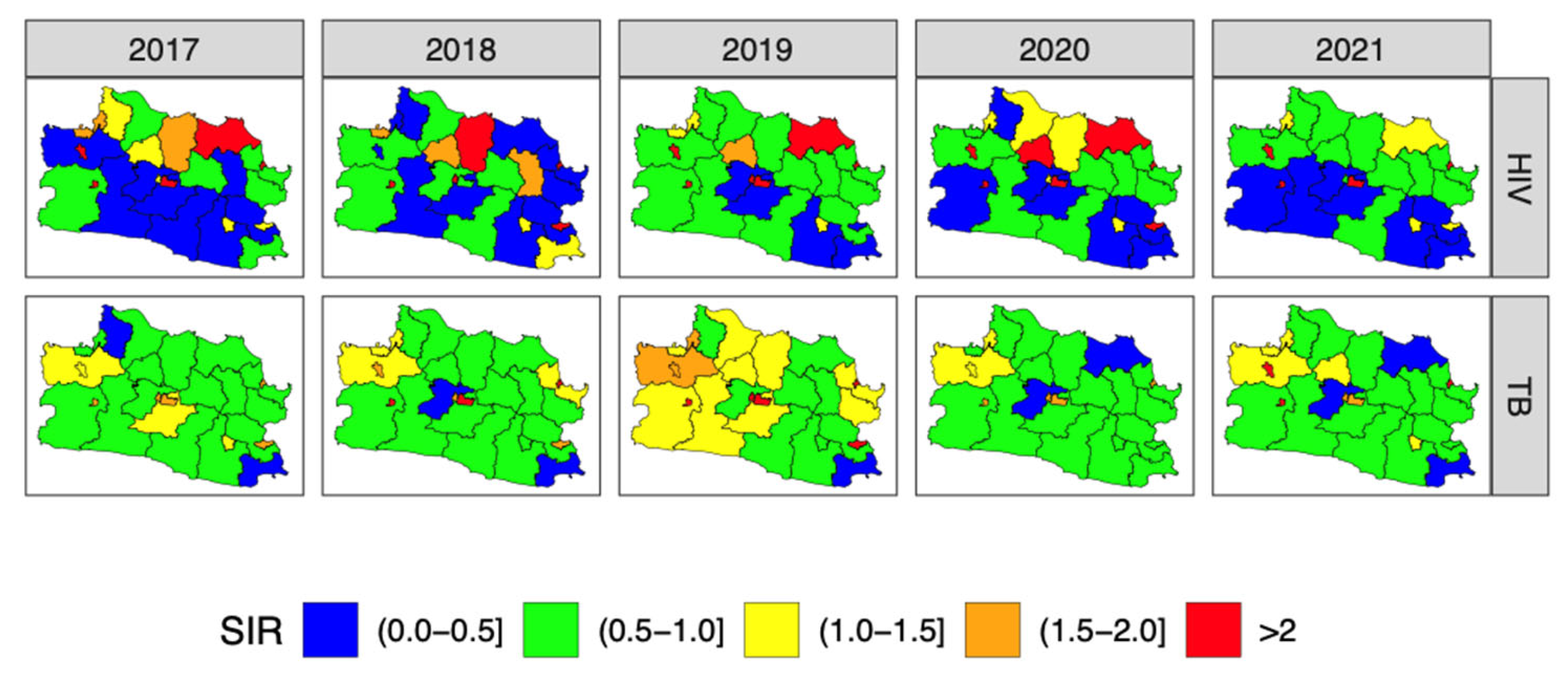
Figure 2 depicts the incidence rate (per 100,000 inhabitants) of HIV and TB in West Java during the study period. Notably, since 2018, there was a significant increase in rates, particularly for HIV and TB. However, while HIV rates were projected to decrease in 2020, TB rates were expected to continue rising. Based on the observed similarities in the temporal rates of HIV and TB over the study period, we hypothesized a potential relationship between the risk of acquiring both diseases. This relationship suggests that certain factors, such as public policies, intervention programs, or laws aimed at preventing the spread of these diseases, may influence this phenomenon. In other words, there are common risk variables that contributed to the spatiotemporal variation in both HIV and TB. This formed the basis for developing a multivariate model with a shared component model approach. For initial identification, we computed the SIR for HIV and TB in 27 districts over 5 years (Figure 3) and assessed the correlation between their spatial and temporal patterns. The summary statistics for these calculations are displayed in Table 2.
The correlations between the spatial distribution patterns (according to year) of HIV and TB ranged from 0.540 to 0.877, with an average of 0.689, suggesting a strong cross-spatial correlation between the two diseases. This indicated that certain areas may share similar risk factors that contribute to both HIV and TB. Additionally, both HIV and TB exhibited a temporal pattern correlation (according to the spatial pattern) ranging from −0.810 to 0.641, with an average close to zero at −0.131, indicating a low cross-temporal correlation between the two diseases. These results provide support for the appropriateness of the spatially shared component in modeling the multivariate semiparametric spatiotemporal model.
To ensure the appropriateness of the data for spatiotemporal modeling and to establish the groundwork for utilizing the area-to-point model with Inverse Distance Weighting (IDW) for generating the high-resolution maps, we conducted calculations of Moran’s I for spatiotemporal autocorrelation, which were validated using a permutation approach. The spatiotemporal computation yielded Moran’s I values of 0.239 (p-value = 0.00) for HIV and 0.683 (p-value = 0.00) for TB. These results represented a significant level of spatiotemporal autocorrelation, particularly in the context of TB. As a result, the conditions were favorable for employing spatiotemporal modeling and interpolation techniques IDW to provide high-resolution maps.

3.2. Model Selection

We evaluated four sub-models, each employing different likelihoods: Poisson and NB for both the parametric and semiparametric models. The goodness of fit of these sub-models was compared using the DIC, WAIC, and MPL criteria. Additionally, we assessed their forecast performance using MAE, RMSE, and R2 with leave-one-out cross-validation. Table 3 presents a summary of the corresponding results. As a rule, the model with the lowest DIC, WAIC, MAE, and RMSE values and the highest MPL and R2 values was considered the most fit and accurate forecast model. Based on Table 3, the variant semiparametric model M2.2, which incorporated the NB probability and RW1 trend, outperformed the other models. M2.2 had a lower DIC (3655), WAIC (3.655), and MAE (0.353) and a higher MPL (−1833) and R2 (0.834). Therefore, we chose the variant semiparametric M2.2 model for further analysis.
To determine whether the M2.2 model was superior at predicting HIV or TB disease, a comprehensive analysis of prediction error magnitudes for each model was conducted. Specifically, the MAE values calculated for HIV and TB were 0.592 and 0.114, respectively. In addition, the RMSE values for HIV and TB were 2.736 and 0.025, respectively. In addition, the R2 for HIV was calculated to be 0.752, while that for TB was significantly higher at 0.953. Collectively, these results demonstrate the M2.2 model’s superior predictive ability in relation to TB compared to HIV. This distinction was due to the significant difference in data volume between tuberculosis and HIV. With significantly more TB data than HIV data, the relative sampling error for TB was significantly reduced, contributing to the model’s improved predictive performance in this context.

3.3. Final Model Inference

Based on the model comparison and selection results, we chose semiparametric model M2.2, which incorporated the combined fixed effect of population density and the spatially and temporally varying effect of the HDI and accounted for the spatially shared effect component. Table 4 presents the summary statistics for fixed effects along with their credibility intervals. As indicated by the credibility intervals, the global log relative risk estimates for HIV and TB were found to be significantly different from zero. Specifically, the relative risk estimates for HIV and TB were less than one, namely 0.629 and 0.735, respectively. This suggests that the relative spatiotemporal risks were primarily influenced by spatial- and temporal-specific effects and spatially shared components. Moreover, we discovered that population density had a positive and statistically significant impact on both HIV and TB. The estimations of relative risk for HIV and TB were 1.140 and 1.075, respectively. This indicates that the transmission of HIV and TB in West Java, Indonesia, is strongly influenced by population density.
Table 5 presents the posterior means of statistics for various factors, including overdispersion, the standard deviation (SD) in spatial shared component effects, and spatially and temporally structured effects of the HDI on HIV and TB risk. The 95% credible intervals are also provided alongside these statistics. The hyperparameter offers insights into the contribution of each fitted random effects toward explaining the relative risk variability. The first noteworthy observation pertains to the overdispersion parameter, which had a value greater than 1, indicating that selecting the NB likelihood was the appropriate choice. The second point of interest is linked to the scale parameter for the spatially shared component. The positive value of the scale parameter δ = 0.5 indicated a positive spatial cross-correlation between HIV and TB risk. A scale values below one suggests that the contribution of spatially shared effects was more significant for HIV than for TB. These findings aligned with the observation that a larger proportion of HIV infections coexisted with TB, while not all TB cases were associated with HIV infection. Next, we considered the spatial autocorrelation associated with the spatially shared component for HIV and TB. A positive value indicated a positive spatial correlation of HIV or TB between areas. This information provides preliminary insights into the existence of spatial clusters for each of the HIV and TB diseases. Additionally, the analysis involved the variance hyperparameter. The percentage of variance indicates that the spatially shared components contributed significantly to the explained variability, accounting for 99.997% of the total variability in HIV and TB risks in comparison to the spatially and temporally varying effects of the HDI. This finding suggests a robust spatial cross-correlation between HIV and TB.
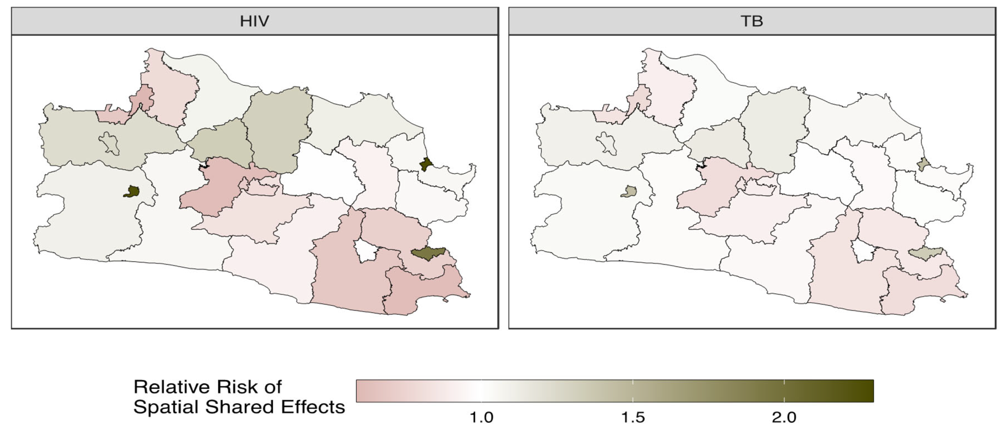
Figure 4 depicts the relative risks associated with the shared spatial patterns. The maps reveal high-risk areas in the northern, eastern, and western parts of West Java, while the central and southeastern regions are characterized by a lower risk. These results suggest that there are shared characteristics in the northern area that act as risk factors and have a similar effect in increasing the risk of both HIV and TB.
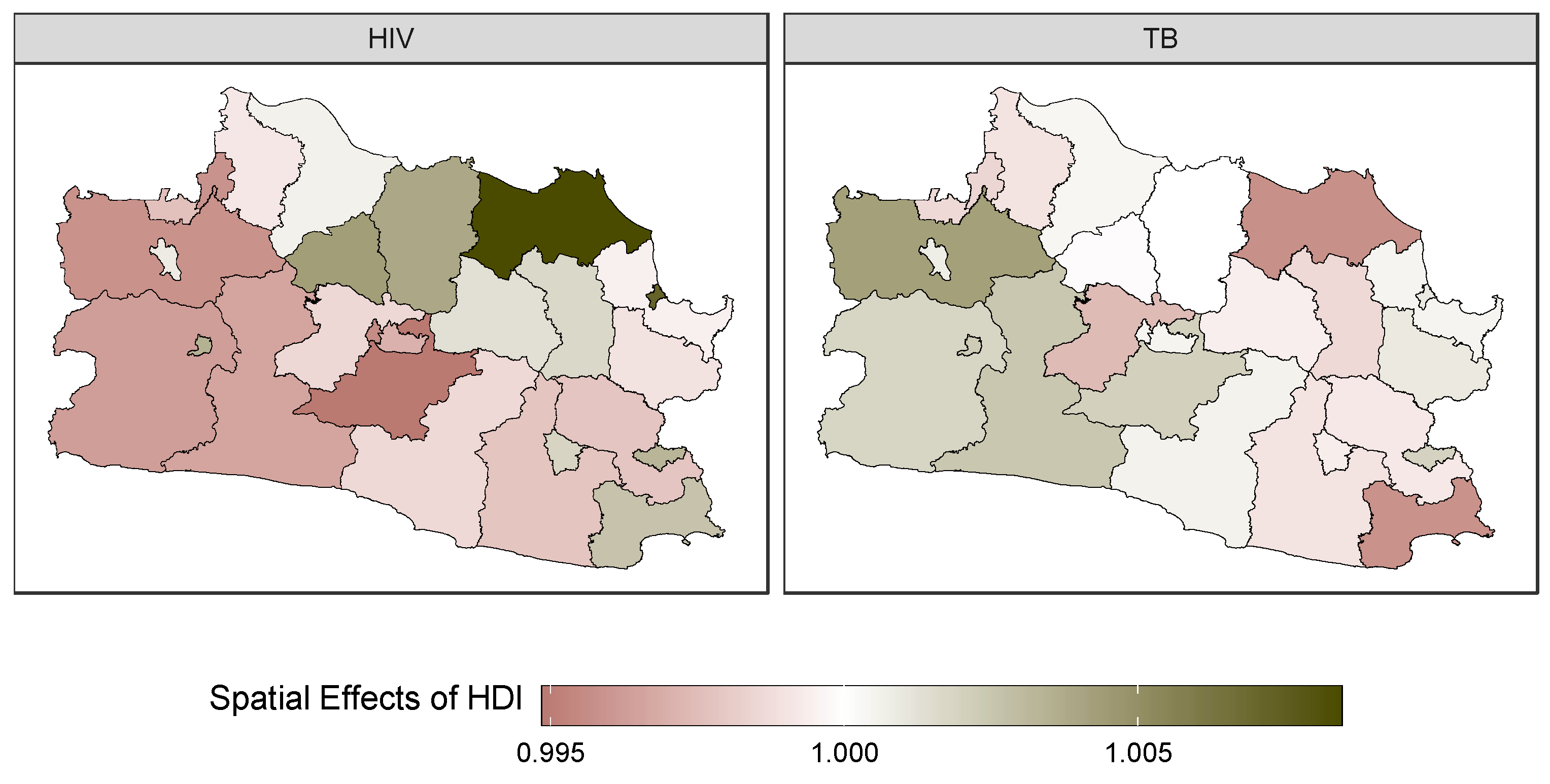
Figure 5 shows the varying spatially structured effects of the HDI on HIV and TB. The spatial effect of the HDI differed between HIV and TB. Specifically, it is evident that the HDI had a positive effect on the areas adjacent to the northeast for HIV. However, for TB, the HDI appeared to exert a tendency toward a negative effect.
Figure 6 illustrates the relative risk associated with the varying temporal structure effects of the HDI. It is noteworthy that the great effect of the HDI on HIV risk occurred in 2018, while for TB, it occurred in 2019. These findings indicate that the effects of the HDI vary considerably over time for both diseases.
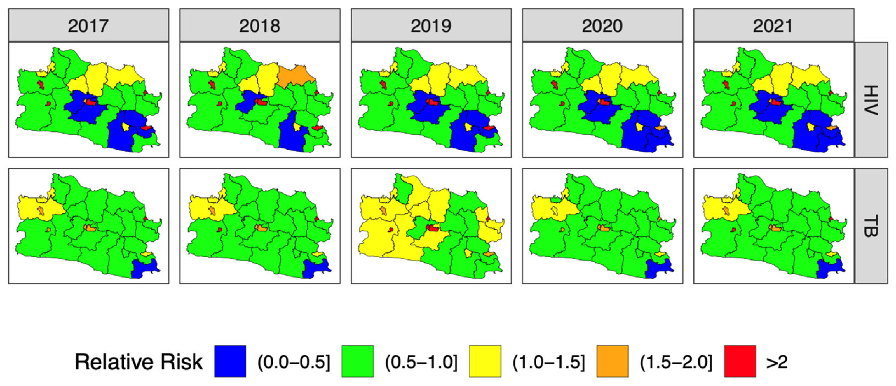
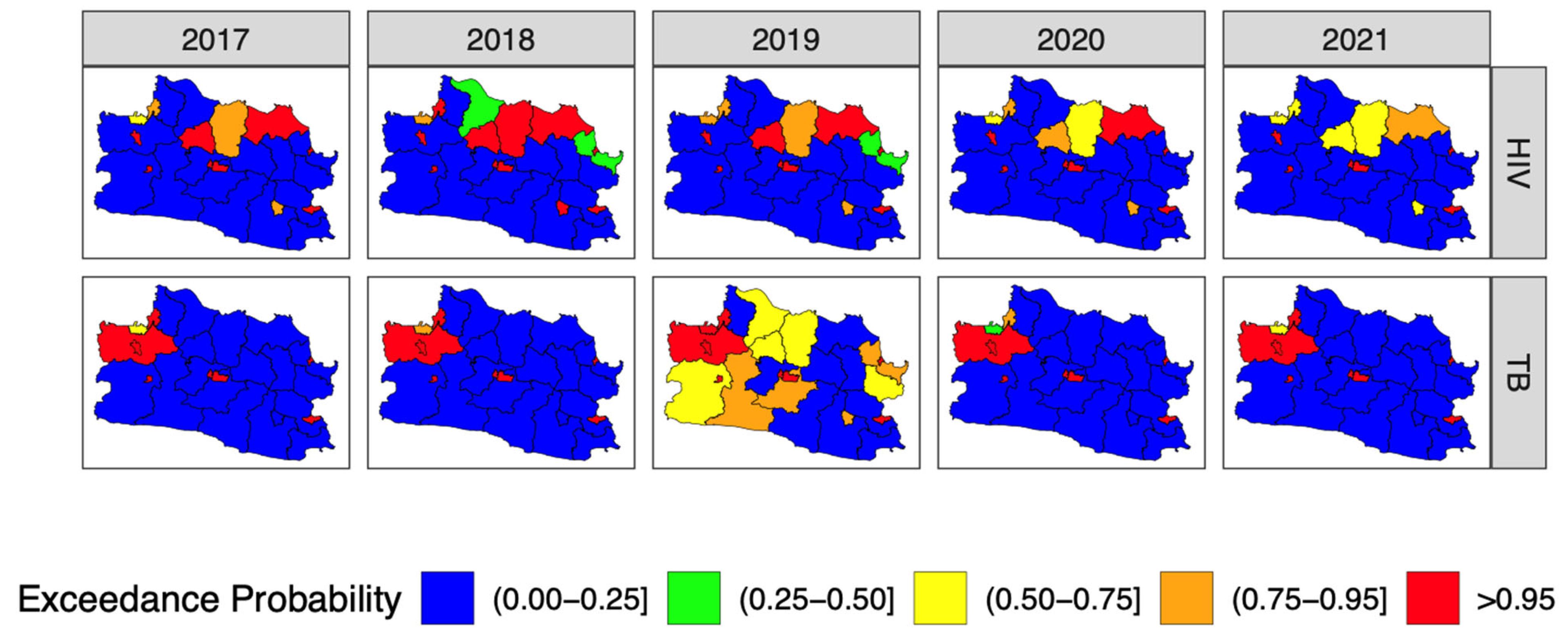
Figure 7 illustrates the estimated relative risk of the combined spatiotemporal HIV and TB patterns, incorporating the combined fixed effects of population density, the spatial and temporal effects of the HDI, and the spatially shared effects. In most areas in West Java, both HIV and TB posed similar low risks. However, HIV showed a high-risk level in most northern areas, while TB exhibited higher risk levels in the northwestern and northern regions of West Java. Interestingly, some areas, such as the Bogor city, Bandung city, Cirebon city, Banjar city, and Sukabumi city districts, were identified as having high- risk levels for both HIV and TB simultaneously. Figure 8 displays the relative risk exceedance probability with a threshold of 1. Most areas were characterized by an exceedance probability value of less than 0.95, indicating that most areas were not hotspot areas. It is important to note that presenting maps as discrete choropleth maps limited by administrative regions can sometimes be challenging to interpret. Hence, we propose presenting the forecasting result in continuous high-resolution maps called isopleth maps.

3.4. Forecasting and High-Resolution Mapping

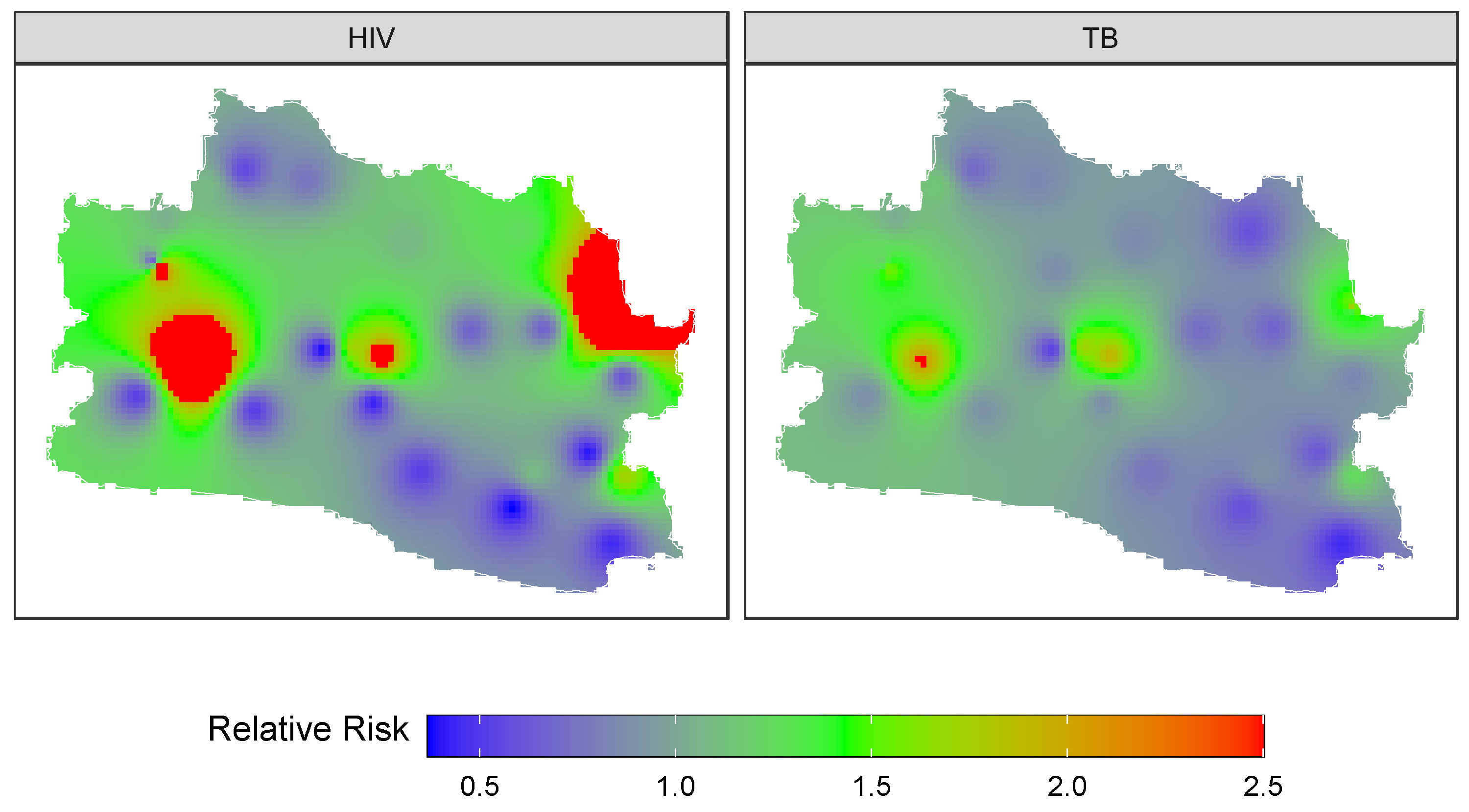
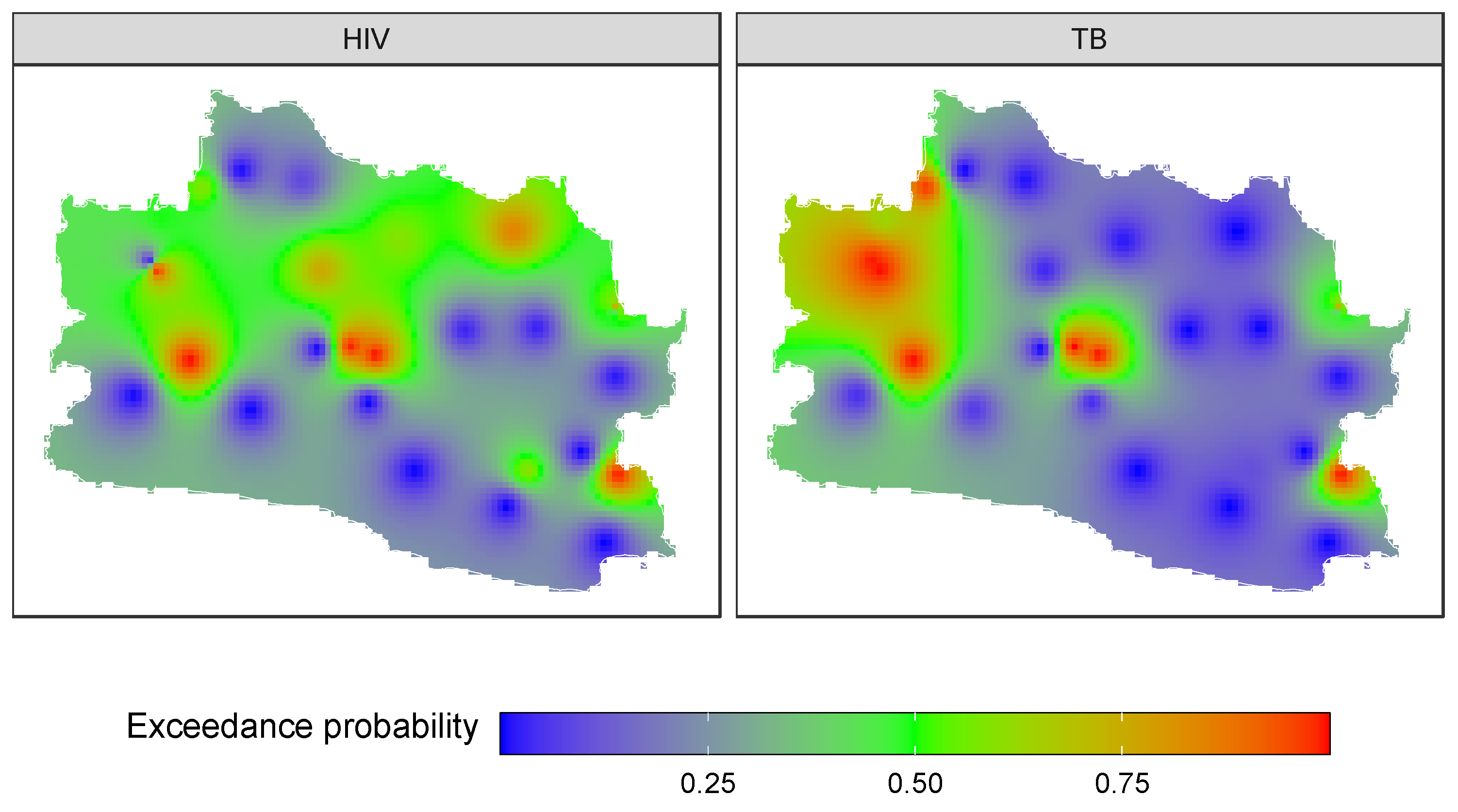
Upon predicting the relative risk and computing the exceedance probability for the period of 2017–2021, our next step involved high-resolution mapping of the forecasted relative risk value for 2022 (Figure 9) as well as the exceedance probability of relative risk for 2022 (Figure 10). By generating high-resolution maps, we aimed to facilitate the interpretation of high-risk forecasting outcomes and identify hotspot areas more effectively.
Based on the observations of Figure 9 and Figure 10, the spatial transmission pattern of HIV and TB was distinctly evident. Hotspots for both diseases were prominently concentrated in the northwestern, central, and southeastern areas that are categorized as urban areas.

4. Discussion

Forecasting and high-resolution mapping for multiple diseases are important tasks in developing an early warning system to target intervention programs and minimize the effects of disease outbreaks [32]. High-resolution maps offer a more accurate representation of disease transmission that is not limited by administrative boundaries. To generate accurate forecasts, the correct model specification is required. A parametric model limits the analysis with strong hypotheses regarding the effect of the covariate on the response variables [28]. However, when there is no clear evidence of the relationship pattern between the predictor and response variables, a semiparametric model could be the best solution [28]. We developed a multivariate Bayesian semiparametric regression model for forecasting and high-resolution mapping. The multivariate Bayesian semiparametric regression model for forecasting and high-resolution mapping was conducted through a two-step approach. We combined Bayesian generalized additive mixed models (GAMMs) and geospatial techniques. A multivariate spatiotemporal model via GAMMs considered shared risk factors in multiple diseases. A geostatistical method through Inverse Distance Weighting (IDW) was utilized to generate a high-resolution risk map based on the forecasting result obtained from the GAMMs.
This methodology was applied to generate forecasts and provide high-resolution maps of HIV and TB risks in West Java, Indonesia. Our working hypothesis was that the semiparametric model would have superior predictive and forecasting abilities when applied to HIV and TB modeling, particularly with respect to predictor variables such as population density and the Human Development Index (HDI). This decision depended on the inherent unpredictability of the potential impact of the HDI on HIV and TB risk. In addition, the influence varied across both spatial and temporal dimensions, demonstrating its inherent contextual nature. This justified the adoption of a framework that allowed the HDI’s effects to vary dynamically in space and time. To rigorously evaluate the relative effectiveness of the semiparametric model versus the parametric model, a sectional model procedure was implemented. This procedure incorporated explicit considerations for model predictions and fit quality. Several criteria were used to evaluate the fitted model, including the Deviance Information Criteria (DIC), the Watanabe Akaike Information Criteria (WAIC), and the Marginal Predicted Likelihood (MPL). In the realm of predictive capabilities, we chose to employ key metrics, including the Mean Absolute Error (MAE), Root Mean Square Error (RMSE), and Coefficient of Determination (R2). These metrics collectively provided a solid evaluation of our model’s predictive ability. Using fit and forecasting criteria, we determined that the semiparametric model with NB likelihood provided the best HIV and TB risk explanation and prediction. We considered semiparametric models and accounted for overdispersion in the count data. We discovered, based on the best model, that an increase in population density within each district was associated with a higher risk of HIV and TB. The Human Development Index (HDI) had varying effects over time and space.
Interestingly, the HDI was found to increase the risk of HIV in certain areas while simultaneously decreasing the risk of TB in those same areas. This spatial heterogeneity effect warrants further investigation to inform efforts for controlling HIV and TB in response to changes in the HDI, which is a composite index that comprises three key indicators: health, education, and the economy. The relationship between the HDI and infectious diseases such as HIV and tuberculosis is a complex mechanism because it involves health, education, and socioeconomic factors that vary across regions and change over time. The progression of the HDI corresponds to improvements in health, education, and community economics. However, significant economic improvements, particularly those geared toward urbanization, can lead to increased migration to urban areas, resulting in a rise in urban population density. Increased population density increases susceptibility to disease transmission, including HIV and tuberculosis. Increasing the HDI, which includes improving education, health, and the economy, must be evenly distributed across all regions over time to decrease the rapid urbanization-induced population density in urban areas. The information obtained is crucial, as interventions must carefully consider the impact of risk variables and socioeconomic inequalities in healthcare. As stated in [64], socioeconomic disparities in healthcare have been proposed as the primary cause of variation in intervention effectiveness. In addition, we found the spatially shared component emerged as the dominant factor, indicating a strong spatial cross-correlation between HIV and TB.
The high-resolution risk and exceedance probability map (Figure 9 and Figure 10) offer valuable insights into the geographical patterns and clusters of disease risk, facilitating targeted interventions and resource allocation. The forecasting outcomes for HIV and TB demonstrated a significant similarity in their patterns. The spatial distribution of HIV and TB indicated high-risk areas in the western, central, northeast, and southeast regions of West Java Province. These regions were identified as hotspots due to their high population density, with Bandung city in the central area being the district with the highest population density in West Java. The forecasting of HIV and TB risks in 2022 that is presented in high-resolution maps suggests that these diseases will display geographical clustering in specific regions of West Java. The observed hotspot clustering in the western, central, northeast, and southeast areas indicated an elevated risk and prevalence of HIV and TB in these regions. Utilizing this information can guide targeted interventions, efficient resource allocation, and informed policy decisions to mitigate disease transmission and enhance public health outcomes.
The validity of high-resolution maps through an area-to-point model employing the Inverse Distance Weighting (IDW) approach was substantiated by the pronounced and statistically significant spatiotemporal autocorrelation observed. However, it is essential to recognize the limitations of this study. Creating a high-resolution map from areal data necessitates first constructing a regression model that combines established data points and uses the values of the areal objects as linear constraints. Second, regional averages exhibit a smaller variance than actual values, making it impractical to fully restore the original variance. These averages are centered around an arbitrary point (centroid), and any change to this point would affect the outcomes. Thirdly, when employing interpolation to create high-resolution maps, one must pay close attention to spatial sampling-reconstruction procedures, in accordance with the Nyquist–Shannon sampling theorem [65]. These factors directly affect the precision of the results. To improve the creation of high-resolution maps in future research, it will be necessary to incorporate relevant predictors at grid points while also resolving the misalignment dilemma caused by the merging of data from different scales. The disintegration of areal unit-derived data into high-resolution grids utilizing block averages, which is facilitated by the Gaussian Markov Random Field [32,34], is an alternative strategy for reducing bias variance and determining the optimal sampling distance. Notably, this method has the potential to reduce inherent biases and achieve the optimal sampling interval. Nevertheless, it is essential to recognize that this method incurs a significant computational burden due to its complexity.

5. Conclusions

We developed a multivariate Bayesian semiparametric regression model for forecasting and high-resolution mapping. We applied this method to develop an early warning system that can effectively and efficiently control HIV and TB transmission simultaneously. By identifying shared spatial patterns between HIV and TB, we were able to gain insights into common risks and generate more accurate forecasts for both diseases. The quantification of HIV and TB covariation improved collaborative disease surveillance and control initiatives. Our findings revealed that population density significantly influences the transmission of both diseases. As population density increases, the risk of HIV and TB transmission also rises considerably across regions. The Human Development Index (HDI) has spatial and temporal effects on the transmission of HIV and TB. However, the spatially and temporally varying effects of the HDI appear distinct between the two diseases.
The applicability of our developed model extends beyond HIV and TB to a wide range of diseases. In actuality, the model can be applied to more than two diseases. By employing the semiparametric multivariate method, researchers can delve deeper into the dynamics of disease transmission and various risk factors, thereby facilitating the development of effective and efficient early warning systems. With its hierarchical structure, the Bayesian approach is an effective method for addressing complex modeling challenges. Notably, the applicability of our model extends beyond epidemiological studies to a variety of geographic investigations.

Author Contributions

Idea formulation, I.G.N.M.J., B.H., Y.A., A.C. and F.K.; methodology, I.G.N.M.J., B.H. and Y.A.; theory, I.G.N.M.J., B.H., Y.A. and M.A.; algorithm design, I.G.N.M.J. and B.H.; result analysis, I.G.N.M.J., B.H. and F.K.; writing, I.G.N.M.J., B.H., Y.A., A.C. and F.K.; reviewing the research, I.G.N.M.J., B.H., Y.A., A.C. and F.K.; supervision; Y.A. and F.K.; project administration, I.G.N.M.J. and M.A.; funding acquisition, M.A. All authors have read and agreed to the published version of the manuscript.

Funding

This research was funded by Direktorat Jenderal Pendidikan Tinggi, Riset, dan Teknologi Kementerian Pendidikan, Kebudayaan, Riset, dan Teknologi (DRTPM: 0217/E5/PG.P2.00/2023) and the Directorate of Research, Community Service, and Innovation (DRPMI: 1834/UN6.3.1/PT.00/2023).

Institutional Review Board Statement

Not applicable.

Informed Consent Statement

Not applicable.

Data Availability Statement

Not applicable.

Acknowledgments

Thanks to the Direktorat Jenderal Pendidikan Tinggi, Riset, dan Teknologi Kementerian Pendidikan, Ke-budayaan, Riset, dan Teknologi and the Directorate of Research, Community Service, and Innovation of Universitas Padjadjaran for providing the research grant program.

Conflicts of Interest

The authors declare no conflict of interest.

Appendix A

Table A1. District identifiers (IDs) of West Java.
IDDistrictIDDistrict
1Regency Bogor14Regency Purwakarta
2Regency Sukabumi15Regency Karawang
3Regency Cianjur16Regency Bekasi
4Regency Bandung17Regency Bandung Barat
5Regency Garut18Regency Pangandaran
6Regency Tasikmalaya19City Bogor
7Regency Ciamis20City Sukabumi
8Regency Kuningan21City Bandung
9Regency Cirebon22City Cirebon
10Regency Majalengka23City Bekasi
11Regency Sumedang24City Depok
12Regency Indramayu25City Cimahi
13Regency Subang26City Tasikmalaya
27City Banjar

References

  1. Coly, S.; Garrido, M.; Abrial, D.; Yao, A.F. Bayesian hierarchical models for disease mapping applied to contagious pathologies. PLoS ONE 2021, 6, e0222898. [Google Scholar] [CrossRef]
  2. MacNab, Y.C. Bayesian disease mapping: Past, present, and future. Spat. Stat. 2022, 50, 100593. [Google Scholar] [CrossRef] [PubMed]
  3. Coly, S.; Charras-Garrido, M.; Abriala, D.; YaoLafourcade, A.F. Spatiotemporal Disease Mapping Applied to Infectious Diseases. Procedia Environ. Sci. 2015, 26, 32–37. [Google Scholar] [CrossRef]
  4. Schrodle, B.; Held, L. Spatio-Temporal Disease Mapping Using INLA. Environmetrics 2011, 22, 725–734. [Google Scholar] [CrossRef]
  5. Otiende, V.A.; Achia, T.N.; Mwambi, H.G. Bayesian Hierarchical Modeling of Joint Spatiotemporal Risk Patterns for Human Immunodeficiency Virus (HIV) and Tuberculosis (TB) in Kenya. PLoS ONE 2020, 15, e0234456. [Google Scholar] [CrossRef]
  6. Baptista, H.; Congdon, P.; Mendes, J.M.; Rodrigues, A.M.; Canhão, H.; Dias, S.S. Disease mapping models for data with weak spatial dependence or spatial discontinuities. Epidemiol. Methods 2020, 9, 20190025. [Google Scholar] [CrossRef]
  7. MacNab, Y.C. On identification in Bayesian disease mapping and ecological−spatial regression models. Stat. Methods Med. Res. 2014, 23, 134–155. [Google Scholar] [CrossRef] [PubMed]
  8. Lawson, A.B. Bayesian Disease Mapping Hierarchical Modeling in Spatial Epidemiology, 3rd ed.; CRC Press: Boca Raton, FL, USA, 2018. [Google Scholar]
  9. Lee, S.A.; Economou, T.; Lowe, R. A Bayesian Modelling Framework to Quantify Multiple Sources of Spatial Variation for Disease Mapping. J. R. Soc. Interface 2022, 19, 20220440. [Google Scholar] [CrossRef]
  10. Chamanpara, P.; Moghimbeigi, A.; Faradmal, J.; Poorolajal, J. Joint Disease Mapping of Two Digestive Cancers in Golestan Province, Iran Using a Shared Component Model. Osong Public Health Res. Perspect. 2015, 6, 205–210. [Google Scholar] [CrossRef]
  11. Manda, S.; Feltbower, R.; Gilthorpe, M. Review and Empirical Comparison of Joint Mapping of Multiple Diseases. S. Afr. J. Epidemiol. Infect. 2012, 27, 169–182. [Google Scholar] [CrossRef]
  12. Held, L.; Natario, I.; Fenton, S.E.; Rue, H.; Becker, N. Towards Joint Disease Mapping. Stat. Methods Med. Res. 2005, 14, 61–82. [Google Scholar] [CrossRef]
  13. Tesema, G.A.; Tessema, Z.T.; Heritier, S.; Stirling, R.G.; Earnest, A. A Systematic Review of Joint Spatial and Spatiotemporal Models in Health Research. Int. J. Environ. Res. Public Health 2023, 20, 5295. [Google Scholar] [CrossRef]
  14. Downing, A.; Forman, D.; Gilthorpe, M.S.; Edwards, K.L.; Manda, S.O. Joint Disease Mapping Using Six Cancers in The Yorkshire Region of England. Int. J. Health Geogr. 2008, 7, 41. [Google Scholar] [CrossRef]
  15. Earnest, A.; Beard, J.R.; Morgan, G.; Lincoln, D.; Summerhayes, R.; Dunn, T.; Muscatello, D.; Mengersen, K. Small Area Estimation of Sparse Disease Counts Using Shared Component Models-Application to Birth Defect Registry Data in New South Wales, Australia. Health Place 2010, 16, 684–693. [Google Scholar] [CrossRef]
  16. Ibáñez-Beroiz, B.; Librero-López, J.; Peiró-Moreno, S.; Bernal-Delgado, E. Shared Component Modelling as an Alternative to Assess Geographical Variations in Medical Practice: Gender Inequalities in Hospital Admissions for Chronic Diseases. BMC Med. Res. Methodol. 2011, 11, 172. [Google Scholar] [CrossRef] [PubMed]
  17. Knorr-Held, L. Bayesian Modelling of Inseparable Space-Time Variation in Disease Risk. Stat. Med. 2000, 19, 2555–2567. [Google Scholar] [CrossRef]
  18. Mahaki, B.; Mehrabi, Y.; Kavousi, A.; Schmid, V.J. Joint Spatio-Temporal Shared Component Model with an Application in Iran Cancer Data. Asian Pac. J. Cancer Prev. 2018, 19, 1553–1560. [Google Scholar] [PubMed]
  19. Meliker, J.R.; Sloan, C.D. Spatio-Temporal Epidemiology: Principles and Opportunities. Spat. Spatio-Temporal Epidemiol. 2011, 2, 1–9. [Google Scholar] [CrossRef]
  20. Richardson, S.; Abellan, J.J.; Best, N. Bayesian Spatio-Temporal Analysis of Joint Patterns of Male and Female Lung Cancer Risks in Yorkshire (UK). Stat. Methods Med. Res. 2006, 15, 385–407. [Google Scholar] [CrossRef]
  21. Oleson, J.J.; Smith, B.J.; Kim, H. Joint Spatio-Temporal Modeling of Low Incidence Cancers Sharing Common Risk Factors. Data Sci. J. 2008, 6, 105–123. [Google Scholar] [CrossRef] [PubMed]
  22. Lee, D. A Comparison of Conditional Autoregressive Models Used in Bayesian Disease Mapping. Spat. Spatio-Temporal Epidemiol. 2011, 2, 79–89. [Google Scholar] [CrossRef]
  23. Giacomini, R.; Kitagawa, T. Robust Bayesian Inference for Set-Identified Models. Econometrica 2021, 89, 1519–1556. [Google Scholar] [CrossRef]
  24. Wasserman, L.A. A Robust Bayesian Interpretation of Likelihood Regions. Ann. Stat. 1989, 17, 1387–1393. [Google Scholar] [CrossRef]
  25. Tzala, E.; Best, N. Bayesian Latent Variable Modelling of Multivariate Spatio-Temporal Variation in Cancer Mortality. Stat. Methods Med. Res. 2007, 97, 97–118. [Google Scholar] [CrossRef]
  26. Banerjee, S.; Carlin, B.P. Semiparametric Spatio-Temporal Frailty Modeling. Environmetrics 2003, 14, 523–535. [Google Scholar] [CrossRef]
  27. Okango, E.; Mwambi, H.; Ngesa, O.; Achia, T. Semi-Parametric Spatial Joint Modeling of HIV and HSV-2 among Women in Kenya. PLoS ONE 2015, 10, e0135212. [Google Scholar] [CrossRef] [PubMed]
  28. Rong, Y.; Zhao, S.D.; Zhu, J.; Yuan, W.; Cheng, W.; Li, Y. More Accurate Semiparametric Regression in Pharmacogenomics. Stat. Interface 2018, 11, 573–580. [Google Scholar] [CrossRef]
  29. Luan, J.; Ba, J.; Liu, B.; Xu, X.; Shu, D. 2021–2022 Monitoring, Early Warning, and Forecasting of Global Infectious Diseases. J. Biosaf. Biosecur. 2022, 4, 98–104. [Google Scholar] [CrossRef]
  30. Wang, A.S. The Early Warning and Forecasting System (EWFS) for the Reduction of Serious Atmosphere-Hydrosphere Disasters. In Early Warning Systems for Natural Disaster Reduction; Zschau, J., Küppers, A., Eds.; Springer: Berlin/Heidelberg, Germany, 2003; pp. 399–402. [Google Scholar]
  31. Tchuente, L.A.T.; Stothard, J.R.; Rollinson, D.; Reinhard-Rupp, J. Precision Mapping: An Innovative Tool and Way Forward to Shrink the Map, Better Target Interventions, and Accelerate toward the Elimination of Schistosomiasis. PLoS Negl. Trop. Dis. 2018, 12, e0006563. [Google Scholar] [CrossRef]
  32. Jaya, I.G.N.M.; Folmer, H. Spatiotemporal High-Resolution Prediction and Mapping: Methodology and Application to Dengue Disease. J. Geogr. Syst. 2022, 24, 527–581. [Google Scholar] [CrossRef]
  33. Blangiardo, M.; Cameletti, M. Spatial and Spatio-Temporal Bayesian Models with R-INLA; John Wiley& Sons: Chennai, India, 2015; pp. 105–200. [Google Scholar]
  34. Utazi, C.E.; Thorley, J.; Alegana, V.A.; Ferrari, M.J.; Nilsen, K.; Takahashi, S.; Metcalf, C.J.E.; Lessler, J.; Tatem, A.J. A Spatial Regression Model for the Disaggregation of Areal Unit Based Data to High-Resolution Grids with Application to Vaccination Coverage Mapping. Stat. Methods Med. Res. 2019, 28, 3226–3241. [Google Scholar] [CrossRef] [PubMed]
  35. Haider, M.S.; Salih, S.K.; Hassan, S.; Taniwall, N.J.; Moazzam, M.F.U.; Lee, B.G. Spatial Distribution and Mapping of COVID-19 Pandemic in Afghanistan using GIS Technique. SN Soc. Sci. 2022, 2, 59. [Google Scholar] [CrossRef] [PubMed]
  36. Berke, O. Exploratory Disease Mapping: Kriging the Spatial Risk Function from Regional Count Data. Int. J. Health Geogr. 2004, 3, 18. [Google Scholar] [CrossRef]
  37. Goovaerts, P. Geostatistical Analysis of Disease Data: Accounting for Spatial Support and Population Density in the Isopleth Mapping of Cancer Mortality Risk Using Area-To-Point Poisson Kriging. Int. J. Health Geogr. 2006, 5, 52. [Google Scholar] [CrossRef]
  38. Tobler, W. A Computer Movie Simulating Urban Growth in The Detroit Region. Econ. Geogr. 1970, 46, 234–240. [Google Scholar] [CrossRef]
  39. Yoo, E.H.; Kyriakidis, P.C.; Tobler, W. Reconstructing Population Density Surfaces from Areal Data: A Comparison of Tobler’s Pycnophylactic Interpolation Method and Area-to-Point Kriging. Geogr. Anal. 2010, 42, 78–98. [Google Scholar] [CrossRef]
  40. Jaya, I.G.N.M.; Ruchjana, B.N.; Abdullah, A.S.; Andriyana, Y. Comparison of IDW and GP Models with Application to Spatiotemporal Interpolation of Rainfall in Bali Province, Indonesia. J. Phys. Conf. Ser. 2021, 1722, 012080. [Google Scholar] [CrossRef]
  41. Jaya, I.G.N.M.; Folmer, H. Bayesian Spatiotemporal Mapping of Relative Dengue Disease Risk in Bandung, Indonesia. J. Geogr. Syst. 2020, 22, 105–142. [Google Scholar] [CrossRef]
  42. Berridge, D.M.; Crouchley, R. Multivariate Generalized Linear Mixed Models Using R; CRC Press: Boca Raton, FL, USA, 2011; pp. 1–20. [Google Scholar]
  43. Khazaei, S.; Rezaeian, S.; Baigi, V.; Saatchi, M.; Molaeipoor, L.; Khazaei, Z.; Khazaei, S.; Raza, O. Incidence and Pattern of Tuberculosis Treatment Success Rates in Different Levels of The Human Development Index: A Global Perspective. S. Afr. J. Epidemiol. Infect. 2017, 32, 100–104. [Google Scholar]
  44. Taylan, M.; Demir, M.; Yılmaz, S.; Kaya, H.; Sen, H.S.; Oruc, M.; Icer, M.; Gunduz, E.; Sezgi, C. Effect of Human Development Index Parameters on Tuberculosis Incidence in Turkish Provinces. J. Infect. Dev. Ctries. 2016, 10, 1183–1190. [Google Scholar] [CrossRef]
  45. Zille, A.I.; Werneck, G.L.; Luiz, R.R.; Conde, M.B. Social Determinants of Pulmonary Tuberculosis in Brazil: An Ecological Study. BMC Pulm. Med. 2019, 19, 87. [Google Scholar] [CrossRef]
  46. Maciel, E.M.G.d.S.; Amancio, J.d.S.; Castro, D.B.d.; Braga, J.U. Social Determinants of Pulmonary Tuberculosis Treatment Non-Adherence in Rio de Janeiro, Brazil. PLoS ONE 2018, 13, e0190578. [Google Scholar] [CrossRef]
  47. Jaya, I.G.N.M.; Folmer, H.; Lundberg, L. A joint Bayesian spatiotemporal risk prediction model of COVID-19 incidence, IC admission, and death with application to Sweden. Ann. Reg. Sci. 2022, 1, 1–34. [Google Scholar] [CrossRef] [PubMed]
  48. Mohebbi, M.; Wolfe, R.; Forbes, A. Disease Mapping and Regression with Count Data in the Presence of Overdispersion and Spatial Autocorrelation: A Bayesian Model Averaging Approach. Int. J. Environ. Res. Public Health 2014, 11, 883–902. [Google Scholar] [CrossRef] [PubMed]
  49. Clayton, D.; Kaldor, J. Empirical Bayes Estimates of Age-Standardized Relative Risks for Use in Disease Mapping. Biometrics 1987, 43, 671–681. [Google Scholar] [CrossRef] [PubMed]
  50. Rue, H.; Martino, S.; Chopin, N. Approximate Bayesian Inference for Latent Gaussian Models by Using Integrated Nested Laplace Approximations. J. R. Stat. Soc. B Stat. 2009, 71, 319–392. [Google Scholar] [CrossRef]
  51. Leroux, B.; Lei, X.; Breslow, N. Estimation of Disease Rates in Small Areas: A New Mixed Model for Spatial Dependence. In Statistical Models in Epidemiology, the Environment and Clinical Trials; Halloran, M., Berry, D., Eds.; Springer: New York, NY, USA, 1999; pp. 135–178. [Google Scholar]
  52. Bivand, R.; Gómez-Rubio, V.; Rue, H. Spatial Data Analysis with R-INLA with Some Extensions. J. Stat. Softw. 2015, 63, 1–31. [Google Scholar] [CrossRef]
  53. Gelman, A. Prior Distributions for Variance Parameters in Hierarchical Models. Bayesian Anal. 2006, 1, 515–534. [Google Scholar] [CrossRef]
  54. Osei, F.; Stein, A. Diarrhea Morbidities in Small Areas: Accounting for Non-Stationarity in Sociodemographic Impacts Using Bayesian Spatially Varying Coefficient Modelling. Sci. Rep. 2017, 7, 9908. [Google Scholar] [CrossRef] [PubMed]
  55. Wang, X.; Yue, Y.R.; Faraway, J. Bayesian Regression Modeling with INLA; CRC Press: Boca Raton, FL, USA, 2018; pp. 1–20. [Google Scholar]
  56. Barbulescu, A.; Bautu, A.; Bautu, E. Optimizing Inverse Distance Weighting with Particle Swarm Optimization. Appl. Sci. 2020, 10, 2054. [Google Scholar] [CrossRef]
  57. Gelman, A.; Hwang, J.; Vehtari, A. Understanding Predictive Information Criteria for Bayesian Models. Stat. Comput. 2014, 24, 997–1016. [Google Scholar] [CrossRef]
  58. Watanabe, S. Asymptotic Equivalence of Bayes Cross Validation and Widely Applicable Information Criterion in Singular Learning Theory. J. Mach. Learn. Res. 2010, 11, 3571–3594. [Google Scholar]
  59. West Java. Health Profile of West Java 2017; West Java Health Office: Bandung, Indonesia, 2017; pp. 83–99. [Google Scholar]
  60. West Java. Health Profile of West Java 2018; West Java Health Office: Bandung, Indonesia, 2018; pp. 82–98. [Google Scholar]
  61. West Java. Health Profile of West Java 2019; West Java Health Office: Bandung, Indonesia, 2019; pp. 81–97. [Google Scholar]
  62. West Java. Health Profile of West Java 2020; West Java Health Office: Bandung, Indonesia, 2020; pp. 84–98. [Google Scholar]
  63. West Java. Health Profile of West Java 2021; West Java Health Office: Bandung, Indonesia, 2021; pp. 81–96. [Google Scholar]
  64. Mabaso, M.; Zama, T.; Mlangeni, L.; Mbiza, S.; Mkhize-Kwitshana, Z. Association between the Human Development Index and Millennium Development Goals 6 Indicators in Sub-Saharan Africa from 2000 to 2014: Implications for the New Sustainable Development Goals. J. Epidemiol. Glob. Health 2018, 8, 77–81. [Google Scholar] [CrossRef] [PubMed]
  65. Wang, C.; Li, X.; Xuan, K.; Jiang, Y.; Jia, R.; Ji, J.; Liu, J. Interpolation of Soil Properties from Geostatistical Priors and DCT-Based Compressed Sensing. Ecol. Indic. 2022, 40, 109013. [Google Scholar] [CrossRef]
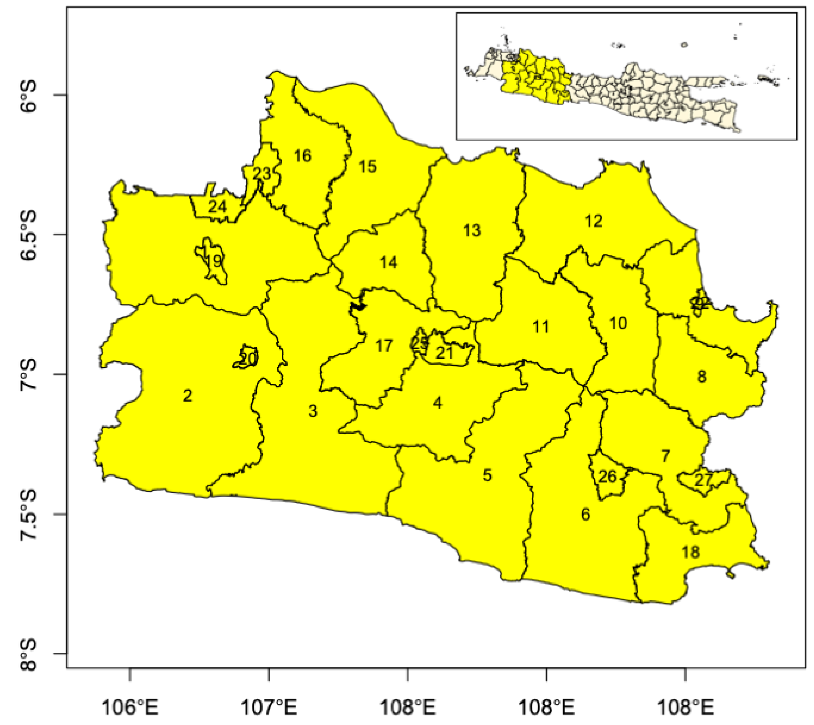
Figure 1. A map showing the administrative districts of West Java and their locations on Java Island, Indonesia (upper right corner). Table A1 in the “Appendix A” provides the district names that correspond to the numbers on the map.
Mathematics 11 03641 g001
Figure 2. Temporal trend incidence rate (per 100,000 inhabitants) of HIV and TB in West Java, Indonesia in 2017–2021.
Mathematics 11 03641 g002
Figure 3. SIR HIV and TB estimated over 2017 to 2021.
Mathematics 11 03641 g003
Figure 4. Estimate of the relative risk of shared spatial pattern of HIV and TB.
Mathematics 11 03641 g004
Figure 5. Estimates of the relative risk of varying spatially structured effects of the HDI on HIV and TB.
Mathematics 11 03641 g005
Figure 6. Estimates of relative risk for varying temporally structured effects of the HDI on HIV and TB.
Mathematics 11 03641 g006
Figure 7. Estimated relative risk of HIV and TB in 2017–2021.
Mathematics 11 03641 g007
Figure 8. Exceedance probability of estimated relative risk in 2017–2021.
Mathematics 11 03641 g008
Figure 9. High-resolution maps of forecasted relative risk for 2022.
Mathematics 11 03641 g009
Figure 10. High-resolution maps of exceedance probability of forecasted relative risk for 2022.
Mathematics 11 03641 g010
Table 1. Descriptive statistics *.
YearHIVTB
MinQ1MeanQ3MaxSDCV (%)MinQ1MeanQ3MaxSDCV (%)
20173385.5217.7292.5986222.8102.33841732.03098.43602.010,9432515.181.2
20183885.0207.5255.01063206.599.53361583.53364.44158.013,5672917.786.7
20194111.0240.1252.01186233.697.33182117.04086.74959.015,8863452.884.5
202016101.5218.0283.5813169.377.73321512.53173.44372.511,1662532.679.8
20214103.5201.6238.5869175.587.12671670.53430.04695.011,9912636.476.9
* Min: Minimum; Q1: 1st Quartile; Q3: 3rd Quartile; Max: Maximum; SD: Standard Deviation; CV: Coefficient of Variation.
Table 2. Pearson’s correlations coefficient between spatial (according to year) and temporal patterns (according to district) of HIV and TB based on standardized incidence ratios (SIRs).
CorrelationMinQ1MeanQ3MaxSDSV
Spatial pattern0.5400.6080.6890.7560.8770.13119.013
Temporal pattern−0.810−0.393−0.1310.1960.6410.419−319.847
Table 3. Model comparison and selection.
ModelLikelihoodDICWAICNPLMAPRMSER2
Parametric models
M1.1Poisson17,81315,184−93660.3711.1870.824
M1.2NB36773678−18460.3721.2100.832
Semiparametric models
M2.1Poisson11,91212,223−67400.3531.2360.824
M2.2NB36553655−18330.3531.1750.834
Table 4. Summary statistics for the fixed effects regression coefficient with their 95% credible intervals.
ParametersMeanSDq(0.025)Medianq(0.975)Relative Risk (RR)
Intercept HIV−0.4630.123−0.703−0.463−0.2210.6294
Intercept TB−0.3080.054−0.413−0.308−0.2030.7349
Population density on HIV0.1310.0310.0700.1310.1911.1400
Population density on TB0.0720.0140.0440.0720.0991.0747
Table 5. Statistics of the posterior means for various factors, including overdispersion, spatial shared component effects, and spatially and temporally structured effects of the HDI on HIV and TB risk. The 95% credible intervals are also provided alongside these statistics.
HyperparametersMeanSDq(0.025)Medianq(0.975)%
Fraction of Variance
Overdispersion parameter for HIV 1 3.7700.4992.8823.7384.835
Overdispersion parameter for TB 2 37.0755.25927.67636.76048.248
Spatial autoregressive of shared component on HIV ( ρ )0.5460.2060.1430.5600.889
Scaling parameter on TB ( δ )0.5000.2490.0390.4881.013
Spatial autoregressive of spatial effect on HIV ( τ 1 )0.4560.2390.0690.4400.903
Spatial autoregressive of spatial effect on TB ( τ 2 )0.3990.1860.1090.3740.797
SD shared component on HIV ( σ ω )0.5850.1870.2830.5651.00899.971
SD temporal effects of HDI on HIV ( σ β 12 )0.0030.0020.0010.0020.0070.002
SD temporal effects of HDI on TB ( σ β 22 )0.0030.0020.0010.0030.0070.003
SD spatial effects of HDI on HIV ( σ β 13 )0.0080.0030.0040.0080.0160.020
SD spatial effects of HDI on TB ( σ β 23 )0.0040.0010.0020.0030.0070.004
Disclaimer/Publisher’s Note: The statements, opinions and data contained in all publications are solely those of the individual author(s) and contributor(s) and not of MDPI and/or the editor(s). MDPI and/or the editor(s) disclaim responsibility for any injury to people or property resulting from any ideas, methods, instructions or products referred to in the content.