Kinetic Behavior and Optimal Control of a Fractional-Order Hepatitis B Model

Abstract

The fractional-order calculus model is suitable for describing real-world problems that contain non-local effects and have memory genetic effects. Based on the definition of the Caputo derivative, the article proposes a class of fractional hepatitis B epidemic model with a general incidence rate. Firstly, the existence, uniqueness, positivity and boundedness of model solutions, basic reproduction number, equilibrium points, and local stability of equilibrium points are studied employing fractional differential equation theory, stability theory, and infectious disease dynamics theory. Secondly, the fractional necessary optimality conditions for fractional optimal control problems are derived by applying the Pontryagin maximum principle. Finally, the optimization simulation results of fractional optimal control problem are discussed. To control the spread of the hepatitis B virus, three control variables (isolation, treatment, and vaccination) are applied, and the optimal control theory is used to formulate the optimal control strategy. Specifically, by isolating infected and non-infected people, treating patients, and vaccinating susceptible people at the same time, the number of hepatitis B patients can be minimized, the number of recovered people can be increased, and the purpose of ultimately eliminating the transmission of hepatitis B virus can be achieved.

1. Introduction

Hepatitis B causes liver lesions, which is an infectious disease caused by the hepatitis B virus. Each outbreak will have a profound impact on human life and health, global social stability, and economic development. Globally, approximately 887,000 people die each year from various diseases associated with hepatitis B infection, with cirrhosis and primary hepatocellular carcinoma accounting for 52 percent and 38 percent of deaths, respectively. Hepatocellular carcinoma can occur in 10 to 25 percent of hepatitis B virus carriers.

Mathematical models are powerful tools for studying the transmission patterns of infectious diseases and finding ways to control their prevalence. It can help us know the dynamics of infectious disease spread and provide some new disease control strategies. Here, we focus on the mathematical model of hepatitis B transmission. Considering that the transmission of hepatitis B is affected by many factors, scholars have established various dynamic models of hepatitis B [1,2,3]. For example, in [4], Khan et al. developed the following hepatitis B model with bilinear incidence:

$$\left\{\begin{array}{c}\frac{dS\left(t\right)}{dt}=\Lambda -\beta S\left(t\right)I\left(t\right)-\left({\mu }_0+\nu \right)S\left(t\right),\hfill \\ \frac{dI\left(t\right)}{dt}=\beta S\left(t\right)I\left(t\right)-\left({\mu }_0+{\mu }_1+\gamma \right)I\left(t\right),\hfill \\ \frac{dR\left(t\right)}{dt}=\gamma I\left(t\right)+\nu S\left(t\right)-{\mu }_{0}R\left(t\right),\hfill \end{array}\right.$$

where $\beta$ is the transmission rate. In [5,6,7,8], the authors proposed several types of stochastic models of hepatitis B with standard incidence rates influenced by environmental fluctuations. The extinction, persistence, and ergodic stability distributions of the hepatitis B model were obtained using stochastic Lyapunov general function theory. Khan et al. [9] established a hepatitis B model with saturation incidence in the following form:

$$\left\{\begin{array}{c}\frac{dS\left(t\right)}{dt}=\Lambda -\frac{\beta S\left(t\right)I\left(t\right)}{1+\eta I\left(t\right)}-\left({\mu }_0+\nu \right)S\left(t\right),\hfill \\ \frac{dI\left(t\right)}{dt}=\frac{\beta S\left(t\right)I\left(t\right)}{1+\eta I\left(t\right)}-\left({\mu }_0+{\mu }_1+\gamma \right)I\left(t\right),\hfill \\ \frac{dR\left(t\right)}{dt}=\gamma I\left(t\right)+\nu S\left(t\right)-{\mu }_{0}R\left(t\right),\hfill \end{array}\right.$$

where $\beta$ and $\eta$, respectively, represent the transmission rate of hepatitis B and saturation rates. Stability theory and central manifold theory were used to study the stability behavior and bifurcation phenomena of the model. Furthermore, the optimal control strategy of hepatitis B transmission was studied by applying the optimal control theory.

In the biomedical field, many biological phenomena, such as biomolecular or cellular interactions, population interactions, microbial cultures, cell growth processes, and human immune processes, exhibit fractal geometry, and global correlation, and have memory genetic effects, so that their kinetic behavior cannot be accurately represented by traditional mathematical models of integer-order microequations. Fractional-order derivatives are closely related to fractal and fractional dimensions and have some unique properties, including global correlation, memorability, and heritability, which make fractional-order differential equation models well suited to describe some complex behaviors and phenomena in nature. Another characteristic of fractional differential equations is that their stability region is larger than that of integer differential equations. This implies that the instability of integer-order differential systems may be stable in fractional differential systems. The fractional-order differential model requires only a few parameters to achieve very good results, solving the defect that the theory of the integer-order differential model does not match well with the experimental results. Therefore, fractional differential equation theory has been widely used to study the modeling of various infectious diseases [10,11,12]. For example, in [13], the authors developed a fractional-order typhoid disease dynamics model. Using the Lyapunov function, the local and global stability of the model was studied. In [14], the authors developed a fractional mathematical model of COVID-19. The uniqueness, boundedness, and non-negativity of the model solutions were discussed. The kinetics and sensitivity analysis were also studied. However, some research methods in integer-order infectious disease dynamics models cannot be directly applied to fractional-order infectious disease dynamics models, and related extensions are being improved. At present, although few differential equations are using fractional-order derivatives to construct models of hepatitis B, more and more scholars have carried out research on fractional-order hepatitis B infectious disease models and achieved certain results. From reading the literature, it is clear that to model the hepatitis B transmission process, some scholars use bilinear incidence rates, standardized incidence rates, and saturation rates. For example, several types of fractional-order hepatitis B transmission models with bilinear incidence rates have been developed in the literature [15,16]. Simelane et al. [17] extended the work of the literature [9] on integer-order hepatitis B models and developed a class of hepatitis B models with Caputo-type fractional-order derivatives as follows:

$$\left\{\begin{array}{c}{}_0^C{D}_t^{\alpha }S\left(t\right)=\Lambda -\frac{\beta S\left(t\right)I\left(t\right)}{1+\eta I\left(t\right)}-\left({\mu }_0+\nu \right)S\left(t\right),\hfill \\ {}_0^C{D}_t^{\alpha }I\left(t\right)=\frac{\beta S\left(t\right)I\left(t\right)}{1+\eta I\left(t\right)}-\left({\mu }_0+{\mu }_1+\gamma \right)I\left(t\right),\hfill \\ {}_0^C{D}_t^{\alpha }R\left(t\right)=\gamma I\left(t\right)+\nu S\left(t\right)-{\mu }_{0}R\left(t\right),\hfill \end{array}\right.$$

where $0<\alpha \le 1$, ${}_0^C{D}_t^{\alpha }$ is the left Caputo fractional derivative. The basic properties of the fractional-order model were studied by applying the generalized fractional-order median theorem. Then the stability of the model was studied by applying fractional-order Routh–Hurwitz stability criterion.

In this paper, we investigate a more general incidence than the one mentioned before. Furthermore, we will further extend the work of [17] by developing a class of fractional-order hepatitis B models with a general incidence rate, in the following form:

$$\left\{\begin{array}{c}{}_0^C{D}_t^{\alpha }S\left(t\right)=\Lambda -\frac{\beta S\left(t\right)I\left(t\right)}{f\left(S\left(t\right),I\left(t\right)\right)}-\left({\mu }_0+\nu \right)S\left(t\right),\hfill \\ {}_0^C{D}_t^{\alpha }I\left(t\right)=\frac{\beta S\left(t\right)I\left(t\right)}{f\left(S\left(t\right),I\left(t\right)\right)}-\left({\mu }_0+{\mu }_1+\gamma \right)I\left(t\right),\hfill \\ {}_0^C{D}_t^{\alpha }R\left(t\right)=\gamma I\left(t\right)+\nu S\left(t\right)-{\mu }_{0}R\left(t\right),\hfill \end{array}\right.$$

(1)

with

$$S\left(0\right)=S_0\ge 0,I\left(0\right)=I_0\ge 0,R\left(0\right)=R_0\ge 0,$$

(2)

where $0<\alpha \le 1$, $S\left(t\right)$, $I\left(t\right)$, and $R\left(t\right)$ represent susceptible, infected, and recovered persons, respectively. $f\left(S,I\right)=1+a_{1}S+a_{2}I+a_{3}SI$, $a_1,a_2,a_3\ge 0$. For convenience below, we define:

$$g\left(S,I\right)=\frac{\beta SI}{f\left(S,I\right)}=\frac{\beta SI}{1+a_{1}S+a_{2}I+a_{3}SI}.$$

where $g\left(S,I\right)$ is the incidence rate. In particular, $g(S,I)$ is the general form of mutual interference between S and I, as follows:

(i)

When $a_1=a_2=a_3=0$, $g(S,I)$ becomes the bilinear incidence;

(ii)

When $a_1=a_3=0$ or $a_2=a_3=0$, $g(S,I)$ becomes the saturation incidence;

(iii)

When $a_3=0$, $g(S,I)$ becomes the Beddington–DeAngelis function;

(iv)

When $a_3=a_1{a}_2$, $g(S,I)$ becomes the Crowley–Martin function.

The meanings of the parameters in this article are as follows:

• $\Lambda$: the birth rate;
• $\beta$: infection rate from susceptible population to hepatitis B;
• ${\mu }_0$: the natural mortality rate;
• ${\mu }_1$: the death rate of hepatitis B;
• $\gamma$: the recovery rate of hepatitis B
• $\nu$: hepatitis B vaccine coverage rate.

Next, we make the following assumptions about model (1):

• $\left(A_1\right).$ $N\left(t\right)$ represents the total population and is divided into three components: $S\left(t\right)$ stands for susceptible person; $I\left(t\right)$ stands for people infected with hepatitis B in the population at time t; $R\left(t\right)$ represents individuals who recover from infection and have lifelong immunity.
• $\left(A_2\right).$ All parameters and state variables of the model are non-negative.
• $\left(A_3\right).$ Incidence is set as the nonlinear incidence rate.
• $\left(A_4\right).$ Once successfully vaccinated or cured by treatment, immunity is considered permanent.

The research motivation of this paper is to study a new fractional hepatitis B transmission model with a more general incidence than that studied in the literature above. The dynamic behavior is studied, and the optimal control problem of the fractional-order hepatitis B model is discussed, and thus, the optimal control strategy is given to eliminate the hepatitis B virus. The innovation of this paper lies in the further extension of the work of literature [17]. Ref. [17] studied fractional hepatitis B models with saturation incidence, and this paper studies a fractional hepatitis B model with a more general incidence. Specifically, the work of reference [17] is a special case of this article when $a_1=a_3=0$.

2. Fractional-Order Basic Concepts

This section introduces the knowledge of fractional-order calculus required for the paper.

Definition 1

([18]). The Riemann–Liouville type left-hand and right-hand fractional-order integrals are defined in the following form, respectively:

$${}_{t_0}{I}_t^{\alpha }u\left(t\right)=\frac{1}{\Gamma \left(\alpha \right)}{\int }_{t_0}^t{(t-s)}^{\alpha -1}u\left(s\right)ds,{}_t{I}_T^{\alpha }u\left(t\right)=\frac{1}{\Gamma \left(\alpha \right)}{\int }_t^T{(s-t)}^{\alpha -1}u\left(s\right)ds,\alpha >0.$$

Definition 2

([18]). The Riemann–Liouville type left and right fractional-order derivatives are defined in the following form, respectively:

$${}_{t_0}{D}_t^{\gamma }u\left(t\right)=\frac{d}{dt}{}_{t_0}{D}_t^{\gamma -1}u\left(t\right)=\frac{1}{\Gamma (1-\gamma )}\frac{d}{dt}\left({\int }_{t_0}^t{(t-s)}^{-\gamma }u\left(s\right)ds\right),0\le \gamma <1,$$

$${}_t{D}_T^{\gamma }u\left(t\right)=-\frac{d}{dt}{}_t{D}_T^{\gamma -1}u\left(t\right)=-\frac{1}{\Gamma (1-\gamma )}\frac{d}{dt}\left({\int }_t^T{(s-t)}^{-\gamma }u\left(s\right)ds\right),0\le \gamma <1.$$

Definition 3

([18]). The left-hand and right-hand fractional-order derivatives of the Caputo type are defined in the following form, respectively:

$${}_{t_0}^C{D}_t^{\gamma }u\left(t\right){=}_{t_0}{D}_t^{\gamma -1}{u}^{\prime }\left(t\right)=\frac{1}{\Gamma (1-\gamma )}{\int }_{t_0}^t{(t-s)}^{-\gamma }{u}^{\prime }\left(s\right)ds,0<\gamma <1,$$

$${}_t^C{D}_T^{\gamma }u\left(t\right)={-}_t{D}_T^{\gamma -1}{u}^{\prime }\left(t\right)=-\frac{1}{\Gamma (1-\gamma )}{\int }_t^T{(s-t)}^{-\gamma }{u}^{\prime }\left(s\right)ds,0<\gamma <1.$$

Lemma 1

([18]). Let $t>0$, $n-1<\gamma <n$, $n\in \mathbb{N}$. Then:

$${}_{t_0}^C{D}_t^{\gamma }u\left(t\right)={}_{t_0}{D}_t^{\gamma }u\left(t\right)-\sum _{j=0}^{n-1}\frac{u^j\left(t_0\right)}{\Gamma \left(j-\gamma +1\right)}{\left(t-t_0\right)}^{j-\gamma },$$

$${}_t^C{D}_T^{\gamma }u\left(t\right)={}_t{D}_T^{\gamma }u\left(t\right)-\sum _{j=0}^{n-1}\frac{u^j\left(T\right)}{\Gamma \left(j-\gamma +1\right)}{\left(T-t\right)}^{j-\gamma }.$$

Thus, if $u\left(t_0\right)=u^{\prime }\left(t_0\right)=\cdots =u^{(n-1)}\left(t_0\right)=0,$ then ${}_{t_0}{D}_t^{\gamma }u\left(t\right)={}_{t_0}^C{D}_t^{\gamma }u\left(t\right)$; if $u\left(T\right)=u^{\prime }\left(T\right)=\cdots =u^{(n-1)}\left(T\right)=0$, then ${}_t{D}_T^{\gamma }u\left(t\right)={}_t^C{D}_T^{\gamma }u\left(t\right)$.

Lemma 2

([19]). For $0<\alpha \le 1,$ we have ${}_t^C{D}_T^{\alpha }u\left(t\right)={}_0^C{D}_t^{\alpha }u\left(T-t\right).$

3. Kinetic Analysis of Fractional-Order Hepatitis B Model

3.1. Positivity and Boundedness of Solutions

The following necessary citation is given first.

Lemma 3

([20]). If $u\left(t\right)\in C[t_0,T]$ and ${}_{t_0}^C{D}_t^{\alpha }u\left(t\right)\in C[t_0,T]$, then:

$$u\left(t\right)=u\left(t_0\right)+\frac{1}{\Gamma \left(\alpha \right)}{}_{t_0}^C{D}_t^{\alpha }u\left(s\right)t^{\alpha },0<\alpha \le 1,$$

where $t_0\le s\le t,\forall t\in (t_0,T]$.

Lemma 4

([19]). Let $0<\alpha \le 1$. Suppose $u\left(t\right)\in C[t_0,T]$ and ${}_{t_0}^C{D}_t^{\alpha }u\left(t\right)\in C[t_0,T]$. If ${}_{t_0}^C{D}_t^{\alpha }u\left(t\right)\ge 0,$$\forall t\in (t_0,T)$, then $u\left(t\right)$ is a non-decreasing function for $\forall t\in [t_0,T]$; If ${}_{t_0}^C{D}_t^{\alpha }u\left(t\right)\le 0,$$\forall t\in (t_0,T)$, then $u\left(t\right)$ is a non-increasing function for $\forall t\in [t_0,T]$.

Theorem 1.

Let $(S,I,R)\in \mathsf{\Omega }$ be one solution of models (1)–(2), where:

$$\mathsf{\Omega }=\left\{(S,I,R)\in {\mathbb{R}}_{+}^3:max\left|S\right|,\left|I\right|,\left|R\right|\le A\right\}$$

for sufficiently large A. Then, the closed set:

$$\Pi =\left\{\left(S,I,R\right)\in {\mathbb{R}}_{+}^3:0<N\left(t\right)=S\left(t\right)+I\left(I\right)+R\left(t\right)\le \frac{\Lambda }{{\mu }_0}\right\}$$

is positively invariant for models (1)–(2).

Proof. 

Step 1. The existence and uniqueness of the solutions of (1) are investigate in the region $\mathsf{\Omega }\times (0,+\infty )$. Define a mapping $H\left(X\right)=(H_1\left(X\right),H_2\left(X\right),H_3\left(X\right))$, where:

$$\begin{array}{cc}\hfill & H_1\left(X\right)=\Lambda -\frac{\beta SI}{f\left(S,I\right)}-\left({\mu }_0+\nu \right)S,\hfill \\ \hfill & H_2\left(X\right)=\frac{\beta SI}{f\left(S,I\right)}-\left({\mu }_0+{\mu }_1+\gamma \right)I,\hfill \\ \hfill & H_3\left(X\right)=\gamma I+\nu S-{\mu }_{0}R.\hfill \end{array}$$

(3)

Then:

$$\begin{array}{cc}\hfill & ∥H\left(X\right),H\left(\overline{X}\right)∥=∥H_1\left(X\right)-H_1\left(\overline{X}\right)∥\hfill \\ \hfill & +∥H_2\left(X\right)-H_2\left(\overline{X}\right)∥+∥H_3\left(X\right)-H_3\left(\overline{X}\right)∥\hfill \\ \hfill & =\left|-\frac{\beta SI}{f\left(S,I\right)}-\left({\mu }_0+\nu \right)S+\frac{\beta \overline{S}\overline{I}}{f\left(\overline{S},\overline{I}\right)}+\left({\mu }_0+\nu \right)\overline{S}\right|\hfill \\ \hfill & +\left|\frac{\beta SI}{f\left(S,I\right)}-\left({\mu }_0+{\mu }_1+\gamma \right)I-\frac{\beta \overline{S}\overline{I}}{f\left(\overline{S},\overline{I}\right)}+\left({\mu }_0+{\mu }_1+\gamma \right)\overline{I}\right|\hfill \\ \hfill & +\left|\gamma I+\nu S-{\mu }_{0}R-\gamma \overline{I}-\nu \overline{S}+{\mu }_0\overline{R}\right|\hfill \\ \hfill & \le \left({\mu }_0+2\nu +\frac{\beta }{a_2}\right)\left|S-\overline{S}\right|+\left({\mu }_0+{\mu }_1+2\gamma +\frac{\beta }{a_1}\right)\left|I-\overline{I}\right|+{\mu }_0\left|R-\overline{R}\right|\hfill \\ \hfill & \le N_1∥X-\overline{X}∥,\hfill \end{array}$$

where $N_1=max\left\{{\mu }_0+2\nu +\frac{\beta }{a_2},{\mu }_0+{\mu }_1+2\gamma +\frac{\beta }{a_1},{\mu }_0\right\}$. Thus, $H\left(X\right)$ satisfies the Lipschitz condition. Hence, we obtain that the solution of model (1) on $(0,\infty )$ exists and is unique.

Step 2. we show that $\Pi$ is one positively invariant set. From model (1), one has:

$$\begin{array}{cc}\hfill {}_0^C{D}_t^{\alpha }S\left(t\right)& =\Lambda -\frac{\beta SI}{f\left(S,I\right)}-\left({\mu }_0+\nu \right)S\ge -\frac{\beta SI}{1+a_{1}S+a_{2}I+a_{3}SI}-\left({\mu }_0+\nu \right)S\hfill \\ \hfill & \ge -\frac{\beta SI}{a_{2}I}-\left({\mu }_0+\nu \right)S\ge -\left[\frac{\beta }{a_2}+\left({\mu }_0+\nu \right)\right]S=-C_{1}S,\hfill \end{array}$$

where $C_1=\frac{\beta }{a_2}+\left({\mu }_0+\nu \right)>0$. Thus, $S\left(t\right)\ge S\left(0\right)E_{\alpha ,1}\left(-C_1{t}^{\alpha }\right)$. Since $S\left(0\right)\ge 0$, $S\left(t\right)\ge 0.$ From model (1), we obtain:

$${}_0^C{D}_t^{\alpha }I\left(t\right)=\frac{\beta SI}{f\left(S,I\right)}-\left({\mu }_0+{\mu }_1+\gamma \right)I\ge -\left({\mu }_0+{\mu }_1+\gamma \right)I=-C_{2}I,$$

where $C_2={\mu }_0+{\mu }_1+\gamma >0$. Since $I\left(0\right)\ge 0$, then $I\left(t\right)\ge I\left(0\right)E_{\alpha ,1}\left(-C_2{t}^{\alpha }\right)\ge 0.$ From model (1), one has:

$${}_0^C{D}_t^{\alpha }R\left(t\right)=\gamma I+\nu S-{\mu }_{0}R\ge -{\mu }_{0}R=-C_{3}R,$$

where $C_3={\mu }_0>0$. Since $R\left(0\right)\ge 0$, then $R\left(t\right)\ge R\left(0\right)E_{\alpha ,1}\left(-C_3{t}^{\alpha }\right)\ge 0.$ Thus, it has been proved that the solutions of (1) are non-negative. According to Lemma 4, the solution of model (1) is still in $\Pi$. From model (1), we get ${}_0^C{D}_t^{\alpha }N\left(t\right)=\Lambda -{\mu }_{0}N-{\mu }_{1}I\le \Lambda -{\mu }_{0}N.$ Then:

$$0\le N\left(t\right)\le N\left(0\right)E_{\alpha }\left(-{\mu }_0{t}^{\alpha }\right)+\Lambda t^{\alpha }{E}_{\alpha ,\alpha +1}\left(-{\mu }_0{t}^{\alpha }\right),\forall t\ge 0.$$

Thus, $\underset{t\to \infty }{\mathrm{limsup}}N\left(t\right)\le \frac{\Lambda }{{\mu }_0}.$ Therefore, all feasible solutions of model (1) are in $\Pi$. That is, $N\left(t\right)$ is bounded by $\frac{\Lambda }{{\mu }_0}$. Thus, all solutions of model (1) are in $\Pi$ for all $t\ge 0$. □

3.2. Equilibrium Points and Their Asymptotic Stability

3.2.1. Disease-Free Equilibrium Point $E^0$ and Stability

Let ${}_0^C{D}_t^{\alpha }S\left(t\right)=0,{}_0^C{D}_t^{\alpha }I\left(t\right)=0,{}_0^C{D}_t^{\alpha }R\left(t\right)=0$, then:

$$E^0=(S^0,I^0,R^0)=\left(\frac{\Lambda }{{\mu }_0+\nu },0,\frac{\nu \Lambda }{\left({\mu }_0+\nu \right){\mu }_0}\right).$$

Let $X=(S,I,R)$, then model (1) can be written in the form: $\frac{dX}{dt}=\mathcal{F}\left(X\right)-\mathcal{V}\left(X\right),$ where

$$\mathcal{F}\left(X\right)=\left(\begin{array}{c}0\\ \frac{\beta SI}{f\left(S,I\right)}\\ 0\end{array}\right),\mathcal{V}\left(X\right)=\left(\begin{array}{c}-\Lambda +\frac{\beta SI}{f\left(S,I\right)}+\left({\mu }_0+\nu \right)S\\ \left({\mu }_0+{\mu }_1+\gamma \right)I\\ -\gamma I-\nu S+{\mu }_{0}R\end{array}\right).$$

(4)

The Jacobian of Equation (4) around $E^0$. Then, the basic reproduction number ${\mathrm{R}}_0$ is the spectral radius of $\mathcal{F}{\mathcal{V}}^{-1}$, in the following form:

$${\mathrm{R}}_0=\frac{\beta \Lambda }{\left({\mu }_0+\nu +a_1\Lambda \right)\left({\mu }_0+{\mu }_1+\gamma \right)}.$$

Theorem 2.

If ${\mathrm{R}}_0<1$, then $E^0$ is locally asymptotically stable, and conversely if ${\mathrm{R}}_0>1$, then $E^0$ is unstable.

Proof. 

The Jacobian matrix of hepatitis B epidemic model (1) at $E^0$ has the following form:

$$J{|}_{E^0}=\left(\begin{array}{ccc}-\left({\mu }_0+\nu \right)& \frac{\beta \Lambda }{{\mu }_0+\nu +a_1\Lambda }& 0\\ 0& \frac{\beta \Lambda }{{\mu }_0+\nu +a_1\Lambda }-\left({\mu }_0+{\mu }_1+\gamma \right)& 0\\ \nu & \gamma & -{\mu }_0\end{array}\right).$$

After calculation, $J{|}_{E^0}$ has three eigenvalues:

$${\lambda }_1=-\left({\mu }_0+\nu \right)<0,{\lambda }_2=-{\mu }_0<0,{\lambda }_3=-\left({\mu }_0+{\mu }_1+\gamma \right)\left(1-{\mathrm{R}}_0\right).$$

If ${\mathrm{R}}_0<1$, then ${\lambda }_3<0$. Therefore, $E^0$ is locally asymptotically stable. On the contrary, if ${\mathrm{R}}_0>1$, then ${\lambda }_3$ is positive, so $E^0$ is an unstable. □

3.2.2. Endemic Equilibrium Point $E^{*}$ and Stability

The calculation leads to $E^{*}=\left(S^{*},I^{*},R^{*}\right)$ in the following form:

$$S^{*}=\frac{\Lambda -t_1{I}^{*}}{t_2},I^{*}=\frac{-{\Delta }_1+\sqrt{{\Delta }_1^2-4t_1^2{a}_3{\Delta }_2}}{2t_1^2{a}_3},R^{*}=\frac{\gamma I^{*}+\nu S^{*}}{{\mu }_0},$$

where $t_1={\mu }_0+{\mu }_1+\gamma ,t_2={\mu }_0+\nu ,{\Delta }_1=t_1^2{a}_1-\Lambda t_1{a}_3-t_1{t}_2{a}_2-\beta t_1,{\Delta }_2=\beta \Lambda -t_1{t}_2-\Lambda t_1{a}_1.$

Lemma 5.

If ${\mathrm{R}}_0>1$, then $E^{*}$ exists.

Proof. 

If ${\mathrm{R}}_0>1$, we have:

$$\begin{array}{cc}\hfill {\Delta }_1& =t_1^2{a}_1-\Lambda t_1{a}_3-t_1{t}_2{a}_2-\beta t_1\hfill \\ \hfill & <\left({\mu }_0+{\mu }_1+\gamma \right)\left[-\left({\mu }_0+\nu \right)\left(\frac{{\mu }_0+{\mu }_1+\gamma }{\Lambda }+a_2\right)-\Lambda a_3\right]<0,\hfill \\ \hfill {\Delta }_2& =\beta \Lambda -t_1{t}_2-\Lambda t_1{a}_1\hfill \\ \hfill & =\left({\mu }_0+\nu +a_1\Lambda \right)\left({\mu }_0+{\mu }_1+\gamma \right)\left({\mathrm{R}}_0^d-1\right)>0.\hfill \end{array}$$

Furthermore, by calculation, we obtain ${\Delta }_1^2-4t_1^2{a}_3{\Delta }_2>0$. Thus, $I^{*}>0.$ Because $2\Lambda t_1{a}_3+{\Delta }_1>\sqrt{{\Delta }_1^2-4t_1^2{a}_3{\Delta }_2}$, so $\Lambda -\frac{-{\Delta }_1+\sqrt{{\Delta }_1^2-4t_1^2{a}_3{\Delta }_2}}{2t_1{a}_3}>0.$ Then, $\Lambda -t_1{I}^{*}>0$. Hence, we have $S^{*}>0$. Thus, $R^{*}>0$. Consequently, $E^{*}$ exists, if ${\mathrm{R}}_0>1$. □

Theorem 3.

If ${\mathrm{R}}_0>1$, then $E^{*}$ is locally asymptotically stable, and conversely, if ${\mathrm{R}}_0<1$, then $E^{*}$ is unstable.

Proof. 

The Jacobian matrix of hepatitis B epidemic model (1) at $E^{*}$ has the following form:

$$J{|}_{E^{*}}=\left(\begin{array}{ccc}-\left({\mu }_0+\nu \right)-\frac{\beta I^{*}\left(1+a_2{I}^{*}\right)}{f^2\left(S^{*},I^{*}\right)}& -\frac{\beta S^{*}\left(1+a_1{S}^{*}\right)}{f^2\left(S^{*},I^{*}\right)}& 0\\ \frac{\beta I^{*}\left(1+a_2{I}^{*}\right)}{f^2\left(S^{*},I^{*}\right)}& \frac{\beta S^{*}\left(1+a_1{S}^{*}\right)}{f^2\left(S^{*},I^{*}\right)}-\left({\mu }_0+{\mu }_1+\gamma \right)& 0\\ \nu & \gamma & -{\mu }_0\end{array}\right).$$

Obviously, ${\lambda }_1=-{\mu }_0<0$. The other two eigenvalues are calculated below. Let:

$$A=\left(\begin{array}{cc}-\left({\mu }_0+\nu \right)-\frac{\beta I^{*}\left(1+a_2{I}^{*}\right)}{f^2\left(S^{*},I^{*}\right)}& -\frac{\beta S^{*}\left(1+a_1{S}^{*}\right)}{f^2\left(S^{*},I^{*}\right)}\\ \frac{\beta I^{*}\left(1+a_2{I}^{*}\right)}{f^2\left(S^{*},I^{*}\right)}& \frac{\beta S^{*}\left(1+a_1{S}^{*}\right)}{f^2\left(S^{*},I^{*}\right)}-\left({\mu }_0+{\mu }_1+\gamma \right)\end{array}\right).$$

By $\frac{dI}{dt}=0$, one has $\frac{\beta S^{*}}{f\left(S^{*},I^{*}\right)}=\left({\mu }_0+{\mu }_1+\gamma \right).$ Thus, $\beta S^{*}=\left({\mu }_0+{\mu }_1+\gamma \right)f\left(S^{*},I^{*}\right)$. By the definition of f, we get $\beta S^{*}\left(1+a_1{S}^{*}\right)<\left({\mu }_0+{\mu }_1+\gamma \right)f^2\left(S^{*},I^{*}\right)$. Thus:

$$\frac{\beta S^{*}\left(1+a_1{S}^{*}\right)}{f^2\left(S^{*},I^{*}\right)}<{\mu }_0+{\mu }_1+\gamma .$$

(5)

Then, by (5), we obtain:

$$\mathrm{trac}\left(A\right)=\left[-\left({\mu }_0+\nu \right)-\frac{\beta I^{*}\left(1+a_2{I}^{*}\right)}{f^2\left(S^{*},I^{*}\right)}\right]+\left[\frac{\beta S^{*}\left(1+a_1{S}^{*}\right)}{f^2\left(S^{*},I^{*}\right)}-\left({\mu }_0+{\mu }_1+\gamma \right)\right]<0$$

and

$$\begin{array}{cc}\hfill \det \left(A\right)=& \left(\left({\mu }_0+\nu \right)+\frac{\beta I^{*}\left(1+a_2{I}^{*}\right)}{f^2\left(S^{*},I^{*}\right)}\right)\left(\left({\mu }_0+{\mu }_1+\gamma \right)-\frac{\beta S^{*}\left(1+a_1{S}^{*}\right)}{f^2\left(S^{*},I^{*}\right)}\right)\hfill \\ \hfill & +\frac{\beta S^{*}\left(1+a_1{S}^{*}\right)}{f^2\left(S^{*},I^{*}\right)}·\frac{\beta I^{*}\left(1+a_2{I}^{*}\right)}{f^2\left(S^{*},I^{*}\right)}>0.\hfill \end{array}$$

Thus, $\mathrm{trac}\left(A\right)<0,\det \left(A\right)>0$ when ${\mathrm{R}}_0>1$. According to the Routh–Hurwitz criterion, the two eigenvalues of the matrix A are negative, so $E^{*}$ is locally asymptotically stable when ${\mathrm{R}}_0>1$. □

3.3. Numerical Simulation

Example 1.

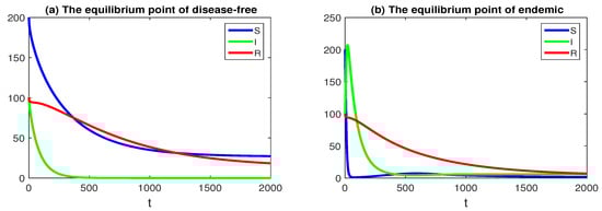
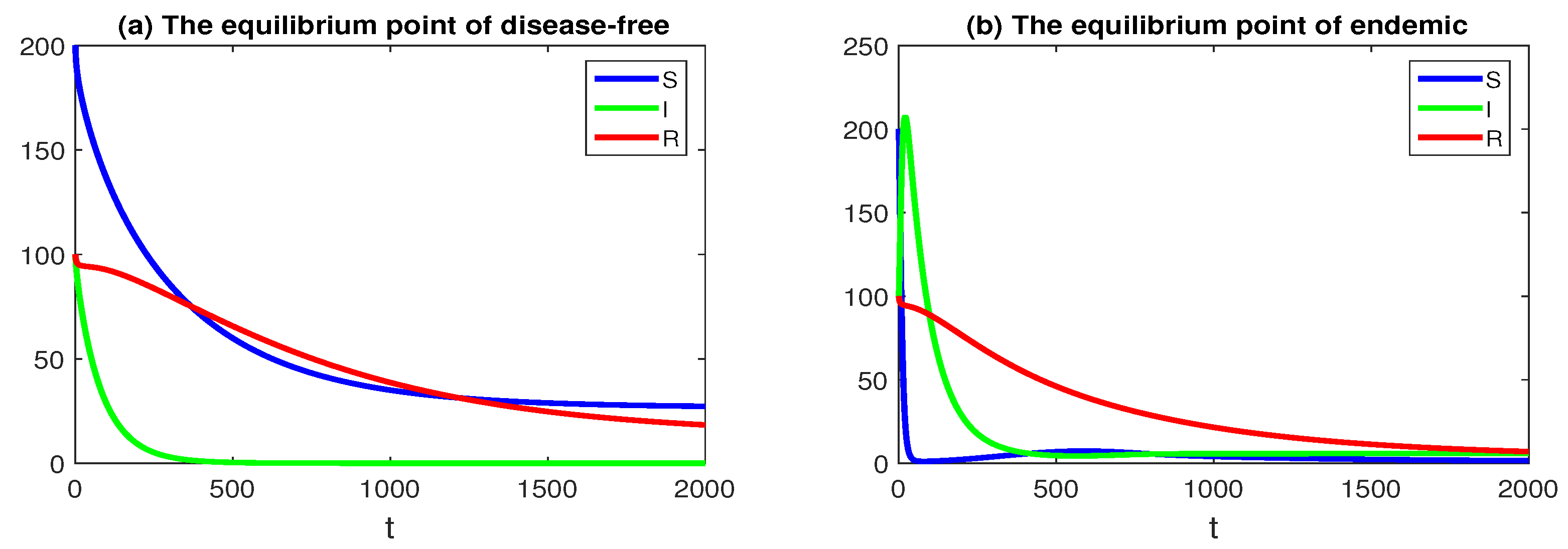
In model (1), let $\alpha =0.98$, $\Lambda =0.8,\beta =0.01,a_1=0.1,a_2=0.2,a_3=1.2,{\mu }_0=0.02,{\mu }_1=0.1,\nu =0.01,\gamma =0.01$, $S\left(0\right)=200,$ $I\left(0\right)=100,$ $R\left(0\right)=100.$ After the calculation, we obtain $E^0=(27,0,13)$ and ${\mathrm{R}}_0=0.56<1$. By observing Figure 1a, we can see that $E^0$ is locally asymptotically stable, which verifies the rationality of Theorem 2.

Figure 1. The plot results show the equilibrium points of the model (1).

Example 2.

See Example 1 for the values of all parameters except $\beta =0.9$. After calculation, we obtain $E^{*}=(5,5,10)$ and ${\mathrm{R}}_0=50>1$. By observing Figure 1b, we can see that $E^{*}$ is locally asymptotically stable, which verifies the rationality of Theorem 3.

4. Optimal Control Analysis

Our aim is to find an effective control strategy to reduce hepatitis B transmission. Optimal control theory [21,22,23] is adopted in this section. The number of hepatitis B patients is reduced by three control variables $u_1\left(t\right)$, $u_2\left(t\right)$, and $u_3\left(t\right)$. The specific explanation of the control variables is as follows:

(i).

$u_1\left(t\right)$ represents the isolation rate. Through this control variable, infected persons are isolated to avoid contact between infected persons and susceptible persons;

(ii).

$u_2\left(t\right)$ represents the cure rate. Through this control variable, the number of infected individuals can be reduced by using effective drugs to treat the infected;

(iii).

$u_3\left(t\right)$ represents vaccination rate. The spread of Hepatitis B can be reduced through vaccination.

To design a control strategy to eliminate hepatitis B, we will consider the optimal strategy of model (1). The control strategy is to minimize the following objective function:

$$J\left(u_1,u_2,u_3\right)={}_0{I}_T^{\alpha }\left[{\omega }_{1}I\left(t\right)+\frac{1}{2}\left({\omega }_2{u}_1^2\left(t\right)+{\omega }_3{u}_2^2\left(t\right)+{\omega }_4{u}_3^2\left(t\right)\right)\right],$$

(6)

subject to the control system:

$$\begin{array}{cc}\hfill & {}_0^C{D}_t^{\alpha }S\left(t\right)=\Lambda -\frac{\beta SI}{f\left(S,I\right)}\left(1-u_1\left(t\right)\right)-\left({\mu }_0+\nu +u_3\left(t\right)\right)S,\hfill \\ \hfill & {}_0^C{D}_t^{\alpha }I\left(t\right)=\frac{\beta SI}{f\left(S,I\right)}\left(1-u_1\left(t\right)\right)-\left({\mu }_0+{\mu }_1+\gamma +u_2\left(t\right)+u_3\left(t\right)\right)I,\hfill \\ \hfill & {}_0^C{D}_t^{\alpha }R\left(t\right)=\left(\gamma +u_2\left(t\right)+u_3\left(t\right)\right)I+\left(\nu +u_3\left(t\right)\right)S-{\mu }_{0}R,\hfill \end{array}$$

(7)

with

$$S\left(0\right)\ge 0,I\left(0\right)\ge 0,R\left(0\right)\ge 0.$$

(8)

In formula (6), ${\omega }_1$ represents the weight constant of hepatitis B infection $I\left(t\right)$, ${\omega }_2$, ${\omega }_3$, and ${\omega }_4$ denote the weight constants for isolation of infected and susceptible individuals, treatment of infected individuals and vaccination, respectively. $\frac{1}{2}{\omega }_2{u}_1^2\left(t\right)$, $\frac{1}{2}{\omega }_3{u}_2^2\left(t\right)$, and $\frac{1}{2}{\omega }_4{u}_3^2\left(t\right)$ represent the costs of isolation, treatment, and vaccination, respectively. Our goal is to search the control functions $u_1^{*},u_2^{*},u_3^{*}$ so that:

$$J\left(u_1^{*},u_2^{*},u_3^{*}\right)=min\left\{J\left(u_1,u_2,u_3\right),u_1,u_2,u_3\in U\right\}$$

(9)

subject to problem (7)–(8), where

$$U:=\left\{\left.\left(u_1,u_2,u_3\right)\right|0\le u_i\le 1,u_i\left(t\right)\mathrm{is}\mathrm{Lebesgue}\mathrm{measurable}\mathrm{on}[0,T],i=\overline{1,3}\right\}.$$

(10)

By applying Pontryaginâs maximum principle in [24] and the results in [25], the following theorem can be obtained.

Theorem 4.

Let $S^{*},I^{*}$, and $R^{*}$ be optimal state solution with associated optimal control variables $\left(u_1^{*},u_2^{*},u_3^{*}\right)$ for the optimal control problems (6)–(7). Then, there are three adjoint variables ${\lambda }_1,{\lambda }_2$, and ${\lambda }_3$ such that:

$$\begin{array}{cc}\hfill {}_0^C{D}_t^{\alpha }{\lambda }_1\left(T-t\right)=& \frac{\beta I^{*}\left(T-t\right)\left(1+a_2{I}^{*}\left(T-t\right)\right)}{f^2\left(S^{*}\left(T-t\right),I^{*}\left(T-t\right)\right)}\hfill \\ \hfill & \times \left({\lambda }_2\left(T-t\right)-{\lambda }_1\left(T-t\right)\right)\left(1-u_1^{*}\left(T-t\right)\right)\hfill \\ \hfill & -\left({\lambda }_1\left(T-t\right)-{\lambda }_3\left(T-t\right)\right)u_3^{*}\left(T-t\right)\hfill \\ \hfill & -{\lambda }_1\left(T-t\right)\left({\mu }_0+\nu \right)+{\lambda }_3\left(T-t\right)\nu ,\hfill \\ \hfill {}_0^C{D}_t^{\alpha }{\lambda }_2\left(T-t\right)=& {\omega }_1+\frac{\beta S^{*}\left(T-t\right)\left(1+a_1{S}^{*}\left(T-t\right)\right)}{f^2\left(S^{*}\left(T-t\right),I^{*}\left(T-t\right)\right)}\hfill \\ \hfill & \times \left({\lambda }_2\left(T-t\right)-{\lambda }_1\left(T-t\right)\right)\left(1-u_1^{*}\left(T-t\right)\right)\hfill \\ \hfill & -\left({\lambda }_2\left(T-t\right)-{\lambda }_3\left(T-t\right)\right)\left(u_2^{*}\left(T-t\right)+u_3^{*}\left(T-t\right)\right)\hfill \\ \hfill & -{\lambda }_2\left(T-t\right)\left({\mu }_0+{\mu }_1+\gamma \right)+{\lambda }_3\left(T-t\right)\gamma ,\hfill \\ \hfill {}_0^C{D}_t^{\alpha }{\lambda }_3\left(T-t\right)=& -{\lambda }_3\left(T-t\right){\mu }_0\hfill \end{array}$$

(11)

with terminal conditions:

$${\lambda }_i\left(T\right)=0,i=1,2,3.$$

(12)

In addition, the optimal controls variables $u_1^{*},u_2^{*}$, and $u_3^{*}$ have the following specific forms:

$$u_1^{*}=max\left\{min\left\{\frac{\left({\lambda }_2-{\lambda }_1\right)\beta S^{*}{I}^{*}}{f\left(S^{*},I^{*}\right){\omega }_2},1\right\},0\right\},$$

(13)

$$u_2^{*}=max\left\{min\left\{\frac{\left({\lambda }_2-{\lambda }_3\right)I^{*}}{{\omega }_3},1\right\},0\right\},$$

(14)

$$u_3^{*}=max\left\{min\left\{\frac{\left({\lambda }_1-{\lambda }_3\right)S^{*}+\left({\lambda }_2-{\lambda }_3\right)I^{*}}{{\omega }_4},1\right\},0\right\}.$$

(15)

Proof. 

Let $x=\left(S,I,R\right)$, $u=(u_1,u_2,u_3)$. Then, the Lagrangian L is defined as:

$$L\left(x,u\right)={\omega }_{1}I+\frac{1}{2}\left({\omega }_2{u}_1^2+{\omega }_3{u}_2^2+{\omega }_4{u}_3^2\right),$$

(16)

and the related Hamiltonian function H is defined as:

$$H\left(x,u,\lambda \right)=L\left(x,u\right)+\lambda g\left(x,u\right),$$

(17)

where $\lambda =\left({\lambda }_1,{\lambda }_2,{\lambda }_3\right)$, and $g\left(x,u\right)=\left(g_1\left(x,u\right),g_2\left(x,u\right),g_3\left(x,u\right)\right)$ with:

$$\begin{array}{cc}\hfill & g_1\left(x,u\right)=\Lambda -\frac{\beta SI}{f\left(S,I\right)}\left(1-u_1\right)-\left({\mu }_0+\nu +u_3\right)S,\hfill \\ \hfill & g_2\left(x,u\right)=\frac{\beta SI}{f\left(S,I\right)}\left(1-u_1\right)-\left({\mu }_0+{\mu }_1+\gamma +u_2+u_3\right)I,\hfill \\ \hfill & g_3\left(x,u\right)=\left(\gamma +u_2+u_3\right)I+\left(\nu +u_3\right)S-{\mu }_{0}R.\hfill \end{array}$$

(18)

Then, we calculate the following adjoint equations:

$$\begin{array}{cc}\hfill {}_t{D}_T^{\alpha }{\lambda }_1=& \frac{\partial H}{\partial S^{*}}={\lambda }_1\left(-\frac{\beta I^{*}\left(1+a_2{I}^{*}\right)}{f^2\left(S^{*},I^{*}\right)}\left(1-u_1^{*}\right)-\left({\mu }_0+\nu +u_3^{*}\right)\right)\hfill \\ \hfill & +{\lambda }_2\left(\frac{\beta I^{*}\left(1+a_2{I}^{*}\right)}{f^2\left(S^{*},I^{*}\right)}\left(1-u_1^{*}\right)\right)+{\lambda }_3\left(\nu +u_3^{*}\right),\hfill \\ \hfill {}_t{D}_T^{\alpha }{\lambda }_2=& \frac{\partial H}{\partial I^{*}}={\omega }_1+{\lambda }_1\left(-\frac{\beta S^{*}\left(1+a_1{S}^{*}\right)}{f^2\left(S^{*},I^{*}\right)}\left(1-u_1^{*}\right)\right)\hfill \\ \hfill & +{\lambda }_2\left(\frac{\beta S^{*}\left(1+a_1{S}^{*}\right)}{f^2\left(S^{*},I^{*}\right)}\left(1-u_1^{*}\right)-\left({\mu }_0+{\mu }_1+\gamma +u_2^{*}+u_3^{*}\right)\right)\hfill \\ \hfill & +{\lambda }_3\left(\gamma +u_2^{*}+u_3^{*}\right),\hfill \\ \hfill {}_t{D}_T^{\alpha }{\lambda }_3=& \frac{\partial H}{\partial R^{*}}=-{\lambda }_3{\mu }_0,\hfill \end{array}$$

(19)

with terminal conditions:

$${\lambda }_i\left(T\right)=0,i=\overline{1,3}$$

(20)

Using Lemma 1, the equivalent equation can be obtained in the following form:

$$\begin{array}{cc}\hfill {}_t^C{D}_T^{\alpha }{\lambda }_1\left(t\right)=& \frac{\beta I^{*}\left(t\right)\left(1+a_2{I}^{*}\left(t\right)\right)}{f^2\left(S^{*},I^{*}\right)}\left({\lambda }_2\left(t\right)-{\lambda }_1\left(t\right)\right)\left(1-u_1^{*}\left(t\right)\right)\hfill \\ \hfill & -{\lambda }_1\left(t\right)\left({\mu }_0+\nu +u_3^{*}\left(t\right)\right)+{\lambda }_3\left(t\right)\left(\nu +u_3^{*}\left(t\right)\right),\hfill \\ \hfill {}_t^C{D}_T^{\alpha }{\lambda }_2\left(t\right)=& {\omega }_1+\frac{\beta S^{*}\left(t\right)\left(1+a_1{S}^{*}\left(t\right)\right)}{f^2\left(S^{*},I^{*}\right)}\left({\lambda }_2\left(t\right)-{\lambda }_1\left(t\right)\right)\left(1-u_1^{*}\left(t\right)\right)\hfill \\ \hfill & -{\lambda }_2\left(t\right)\left({\mu }_0+{\mu }_1+\gamma +u_2^{*}\left(t\right)+u_3^{*}\left(t\right)\right)+{\lambda }_3\left(t\right)\left(\gamma +u_2^{*}\left(t\right)+u_3^{*}\left(t\right)\right),\hfill \\ \hfill {}_t^C{D}_T^{\alpha }{\lambda }_3\left(t\right)=& -{\lambda }_3\left(t\right){\mu }_0,\hfill \end{array}$$

(21)

where ${}_t^C{D}_T^{\alpha }$ is the fractional-order derivative of the right-hand side Caputo type. By Lemma 2, one has:

$$\begin{array}{cc}\hfill {}_0^C{D}_t^{\alpha }{\lambda }_1\left(T-t\right)=& \frac{\beta I^{*}\left(T-t\right)\left(1+a_2{I}^{*}\left(T-t\right)\right)}{f^2\left(S^{*}\left(T-t\right),I^{*}\left(T-t\right)\right)}\hfill \\ & \times \left({\lambda }_2\left(T-t\right)-{\lambda }_1\left(T-t\right)\right)\left(1-u_1^{*}\left(T-t\right)\right)\hfill \\ \hfill & -\left({\lambda }_1\left(T-t\right)-{\lambda }_3\left(T-t\right)\right)u_3^{*}\left(T-t\right)\hfill \\ \hfill & -{\lambda }_1\left(T-t\right)\left({\mu }_0+\nu \right)+{\lambda }_3\left(T-t\right)\nu ,\hfill \\ \hfill {}_0^C{D}_t^{\alpha }{\lambda }_2\left(T-t\right)=& {\omega }_1+\frac{\beta S^{*}\left(T-t\right)\left(1+a_1{S}^{*}\left(T-t\right)\right)}{f^2\left(S^{*}\left(T-t\right),I^{*}\left(T-t\right)\right)}\hfill \\ \hfill & \times \left({\lambda }_2\left(T-t\right)-{\lambda }_1\left(T-t\right)\right)\left(1-u_1^{*}\left(T-t\right)\right)\hfill \\ \hfill & -\left({\lambda }_2\left(T-t\right)-{\lambda }_3\left(T-t\right)\right)\left(u_2^{*}\left(T-t\right)+u_3^{*}\left(T-t\right)\right)\hfill \\ \hfill & -{\lambda }_2\left(T-t\right)\left({\mu }_0+{\mu }_1+\gamma \right)+{\lambda }_3\left(T-t\right)\gamma ,\hfill \\ \hfill {}_0^C{D}_t^{\alpha }{\lambda }_3\left(T-t\right)=& -{\lambda }_3\left(T-t\right){\mu }_0,\hfill \end{array}$$

(22)

where ${}_0^C{D}_t^{\alpha }$ is the fractional-order derivative of the left-hand side Caputo type. Let $\frac{\partial H}{\partial u_k}=0$, $k=\overline{1,3}$, then we have:

$$\begin{array}{cc}\hfill & \frac{\partial H}{\partial u_1^{*}}={\omega }_2{u}_1^{*}\left(t\right)+\left({\lambda }_1\left(t\right)-{\lambda }_2\left(t\right)\right)\frac{\beta S^{*}{I}^{*}}{f\left(S^{*},I^{*}\right)}=0,\hfill \\ \hfill & \frac{\partial H}{\partial u_2^{*}}={\omega }_3{u}_2^{*}\left(t\right)+\left({\lambda }_3\left(t\right)-{\lambda }_2\left(t\right)\right)I^{*}=0,\hfill \\ \hfill & \frac{\partial H}{\partial u_3^{*}}={\omega }_4{u}_3^{*}\left(t\right)+\left({\lambda }_3\left(t\right)-{\lambda }_1\left(t\right)\right)S^{*}+\left({\lambda }_3\left(t\right)-{\lambda }_2\left(t\right)\right)I^{*}=0.\hfill \end{array}$$

(23)

This achieves the optimality condition $H\left(x^{*},u^{*},\lambda \right)=\underset{u\in \left[0,1\right]}{min}H\left(x^{*},u^{*},\lambda \right).$ By taking into account:

$${\widehat{u}}_1^{*}\left(t\right)=\frac{\beta S^{*}{I}^{*}\left({\lambda }_2\left(t\right)-{\lambda }_1\left(t\right)\right)}{f\left(S^{*},I^{*}\right){\omega }_2},{\widehat{u}}_2^{*}\left(t\right)=\frac{\left({\lambda }_2\left(t\right)-{\lambda }_3\left(t\right)\right)I^{*}}{{\omega }_3},$$

$${\widehat{u}}_3^{*}\left(t\right)=\frac{\left({\lambda }_1\left(t\right)-{\lambda }_3\left(t\right)\right)S^{*}+\left({\lambda }_2\left(t\right)-{\lambda }_3\left(t\right)\right)I^{*}}{{\omega }_4},$$

the optimal value of the objective function can be obtained:

$$u_1^{*}=max\left\{min\left\{{\widehat{u}}_1^{*}\left(t\right),1\right\},0\right\},u_2^{*}=max\left\{min\left\{{\widehat{u}}_2^{*}\left(t\right),1\right\},0\right\},u_3^{*}=max\left\{min\left\{{\widehat{u}}_3^{*}\left(t\right),1\right\},0\right\}.$$

□

5. Numerical Simulation

To test the plausibility of the results, we simulate the hepatitis B model (1). Firstly, a set of discrete knots $t_j=t_0+jh,h=\frac{T-t_0}{N};j=0,1,\dots ,N$ are used to replace the time interval $[t_0,T]$. By the fractional Euler method for model (7), we obtain the following discretized equations:

$$\begin{array}{cc}\hfill & S\left(t_k\right)=S\left(t_0\right)+\frac{h^{\alpha }}{\Gamma \left(\alpha +1\right)}\sum _{j=0}^{k-1}{c}_{j,k}\left[\Lambda -\frac{\beta S\left(t_j\right)I\left(t_j\right)}{f\left(S\left(t_j\right),I\left(t_j\right)\right)}\left(1-u_1\right)-\left({\mu }_0+\nu +u_3\right)S\left(t_j\right)\right],\hfill \\ \hfill & I\left(t_k\right)=I\left(t_0\right)+\frac{h^{\alpha }}{\Gamma \left(\alpha +1\right)}\sum _{j=0}^{k-1}{c}_{j,k}\left[\frac{\beta S\left(t_j\right)I\left(t_j\right)}{f\left(S\left(t_j\right),I\left(t_j\right)\right)}\left(1-u_1\right)-\left({\mu }_0+{\mu }_1+\gamma +u_2+u_3\right)I\left(t_j\right)\right],\hfill \\ \hfill & R\left(t_k\right)=R\left(t_0\right)+\frac{h^{\alpha }}{\Gamma \left(\alpha +1\right)}\sum _{j=0}^{k-1}{c}_{j,k}\left[\left(\gamma +u_2+u_3\right)I\left(t_j\right)+\left(\nu +u_3\right)S\left(t_j\right)-{\mu }_{0}R\left(t_j\right)\right],\hfill \end{array}$$

where $c_{j,k}={\left(k-j\right)}^{\alpha }-{\left(k-1-j\right)}^{\alpha }$, for $k=\overline{1,N}$, $u_1\left(t\right)$ represents the isolation rate, $u_2\left(t\right)$ represents the cure rate, and $u_3\left(t\right)$ represents vaccination rate. We study the effect of $\alpha$ in the absence of isolation measures, vaccination, and treatment (i.e., $u_1=u_2=u_3=0$) on the kinetic behavior of the hepatitis B model (1) with a step size of $=0.1$. We plot all compartments for $\alpha =0.9;0.95;0.98;1$ using the data from Example 1 (see Figure 2).

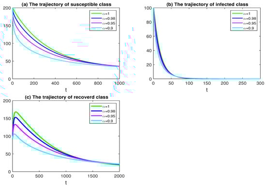
Figure 2. Transient behavior of $\left(S\right(t),I(t),R(t\left)\right)$ in model (7) at different fractional-order derivatives $\alpha =0.9;0.95;0.98;1$.

Figure 2 demonstrates that the curve more closely resembles the integer-order hepatitis B model. As the fractional order $\alpha$ increases, the number of people recovering increases faster and the disease becomes extinct faster.

We also solve numerically the fractional-order optimal control problems (6), (7), and (11) and compare them with the uncontrolled hepatitis B model (1) (see Figure 3, Figure 4, Figure 5, Figure 6, Figure 7, Figure 8 and Figure 9).

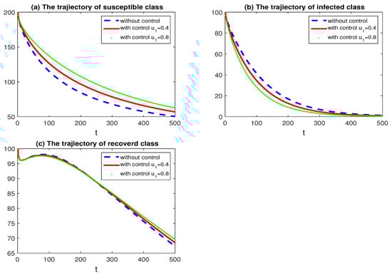
Figure 3. Simulations of $\left(S\right(t),I(t),R(t\left)\right)$ in model (7) with different control $u_1$.

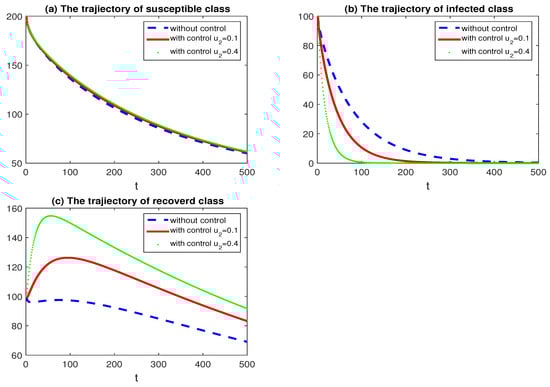
Figure 4. Simulations of $\left(S\right(t),I(t),R(t\left)\right)$ in model (7) with different control $u_2$.

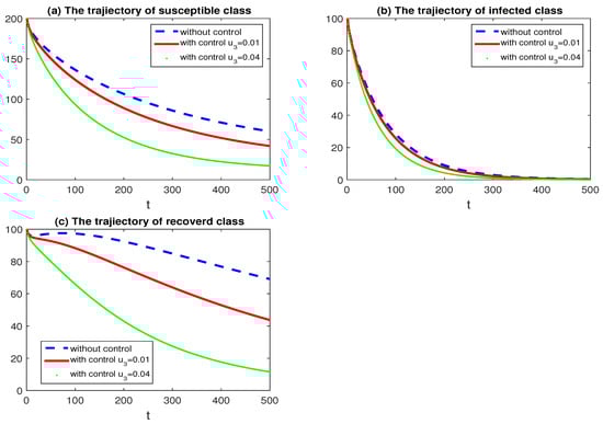
Figure 5. Simulations of $\left(S\right(t),I(t),R(t\left)\right)$ in model (7) with different control $u_3$.

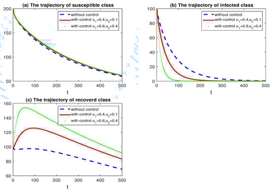
Figure 6. Simulations of $\left(S\right(t),I(t),R(t\left)\right)$ in model (7) with different control pairs $u_1,u_2$.

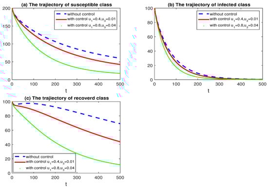
Figure 7. Simulations of $\left(S\right(t),I(t),R(t\left)\right)$ in model (7) with different control pairs $u_1,u_3$.

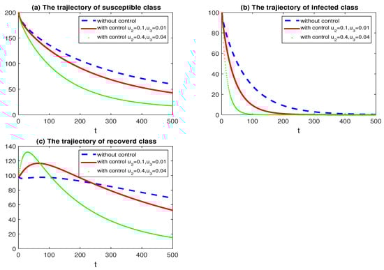
Figure 8. Simulations of $\left(S\right(t),I(t),R(t\left)\right)$ in model (7) with different control pairs $u_2,u_3$.

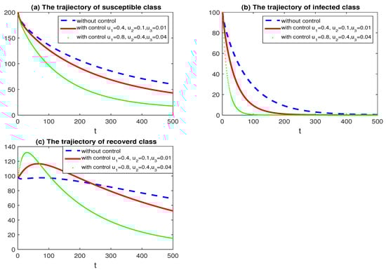
Figure 9. Simulations of $\left(S\right(t),I(t),R(t\left)\right)$ in model (7) with different control pairs $u_1,u_2,u_3$.

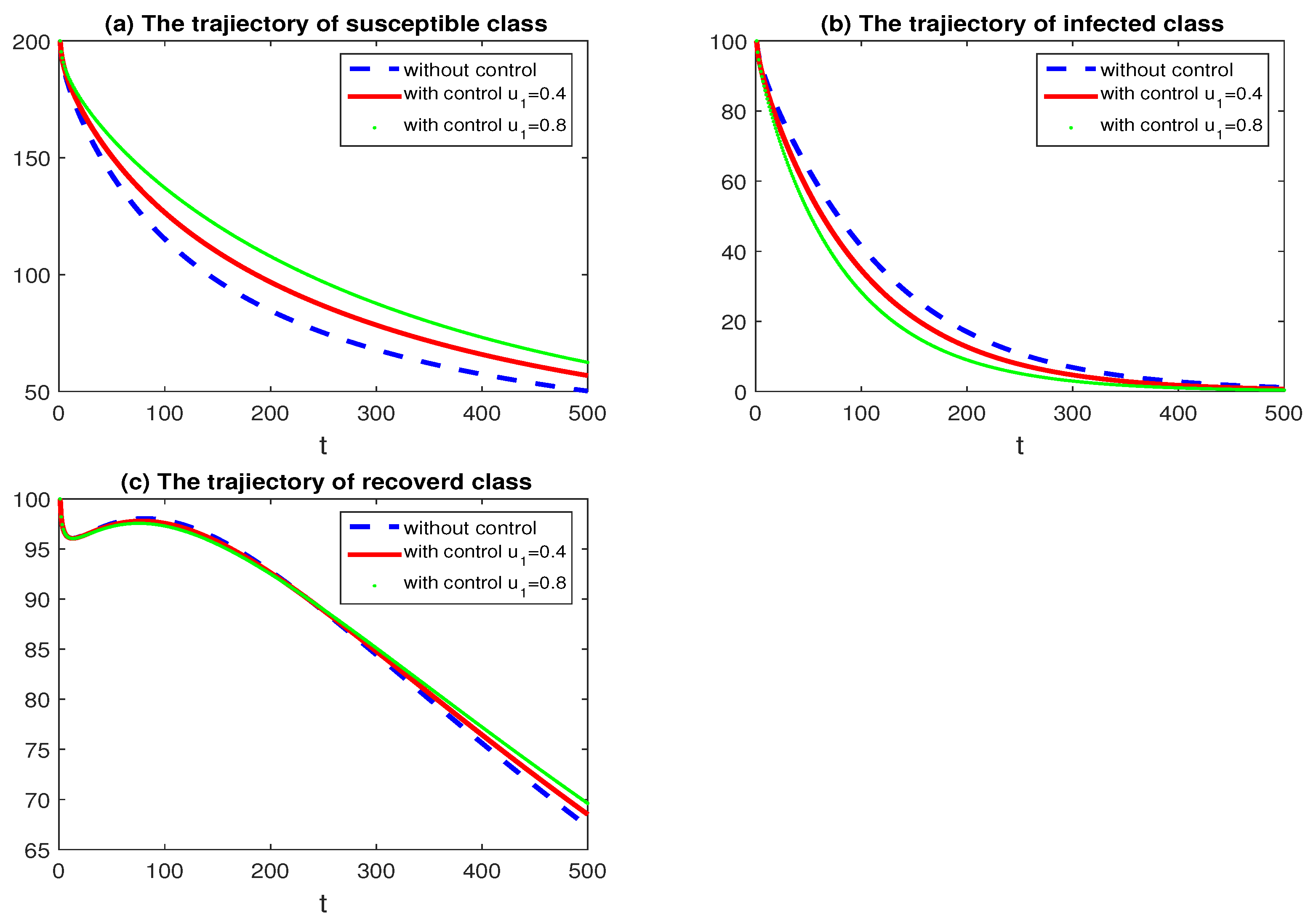
Figure 3 describes the optimal control results of the fractional-order hepatitis B model under the measures of isolating infected persons and avoiding contact between infected and susceptible persons by controlling variable $u_1\left(t\right)$. Figure 3a–c represent the dynamic behavior of susceptible, infected, and recovered persons under isolation measures, respectively. By observing Figure 3, it can be seen that the greater the isolation intensity (i.e., the greater the value of $u_1\left(t\right)$), the faster the decline in the number of infected patients.

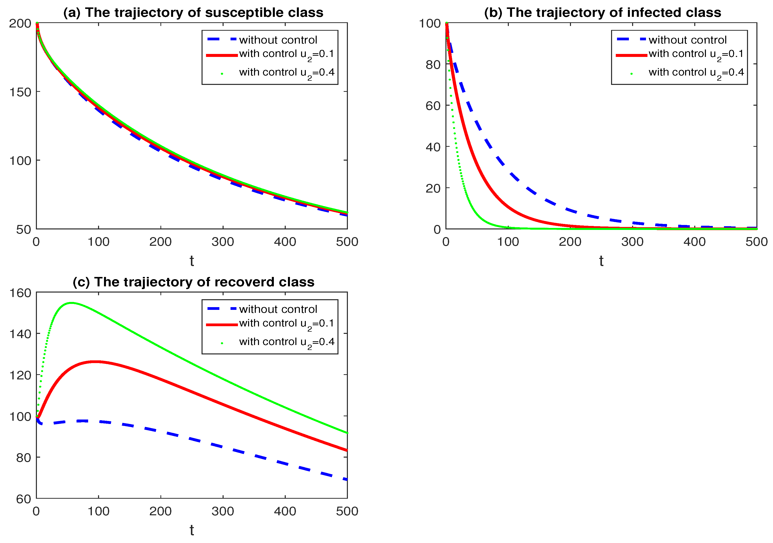
Figure 4 depicts the optimal control results of the fraction-order hepatitis B model under the measure of effective drug treatment of infected persons through the control variable $u_2\left(t\right)$. Figure 4a–c represent the dynamic behavior of susceptible, infected, and recovered persons under effective drug treatment, respectively. By observing Figure 4, it can be seen that the greater the intensity of effective drug treatment for infected patients (i.e., the greater the value of $u_2\left(t\right)$), the faster the number of infected patients will decline and the faster the recovery rate of recovered patients will be.

Figure 5 depicts the optimal control results of the fractional-order hepatitis B model using measures to vaccinate susceptible individuals by controlling variable $u_3\left(t\right)$. Figure 5a–c represent the dynamic behavior of susceptible, infected, and recovered persons under vaccination measures, respectively. From the observation of Figure 5, it can be seen that the greater the intensity of vaccination for susceptible persons (i.e., the greater the value of $u_3\left(t\right)$), the faster the number of susceptible persons will decline, and the faster the number of infected persons will decline.

Figure 6 describes the optimal control results for the fractional hepatitis B model by controlling variables $u_1\left(t\right),u_2\left(t\right)$. Figure 6a–c represent, respectively, the dynamic behavior of susceptible, infected, and recovered persons under simultaneous isolation and effective drug treatment of infected persons. It can be seen from Figure 6 that the greater the intensity of isolation and effective drug treatment for infected patients (i.e., the greater the value of $u_1\left(t\right)$ and $u_2\left(t\right)$), the faster the number of infected patients will decline, and the faster the recovery rate of recovered patients will be.

Figure 7 describes the optimal control results for the fractional hepatitis B model by controlling variables $u_1\left(t\right),u_3\left(t\right)$. Figure 7a–c represent the dynamic behavior of susceptible, infected, and recovered persons, respectively, through simultaneous isolation of infected persons and vaccination of vulnerable populations. It can be seen from Figure 7 that the greater the intensity of isolation of infected persons and vaccination of susceptible persons (i.e., the greater the value of $u_1\left(t\right)$ and $u_3\left(t\right)$), the faster the number of susceptible persons will decline, and the faster the number of infected persons will decline.

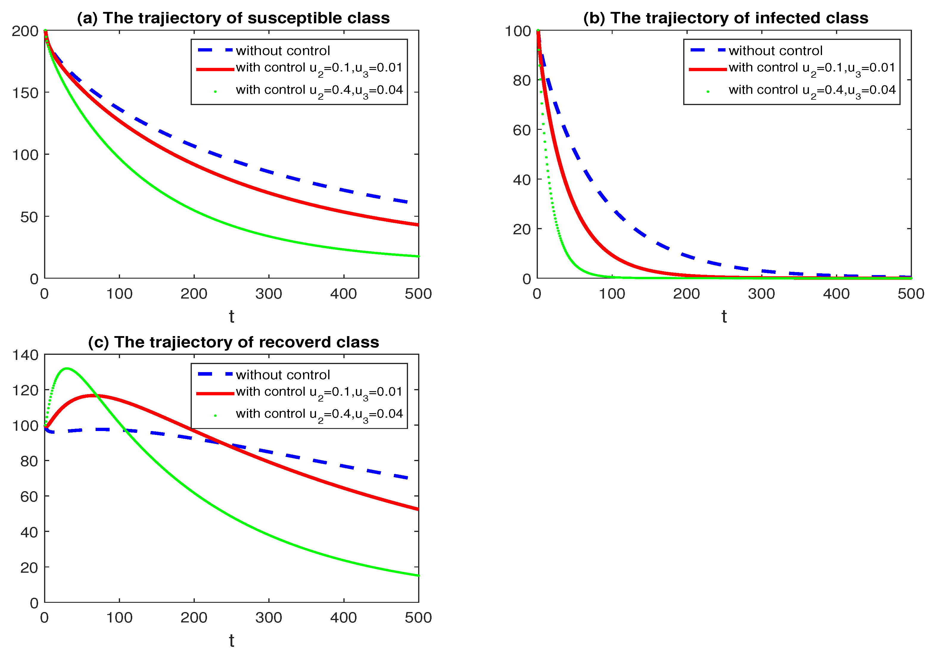
Figure 8 describes the optimal control results for the fractional hepatitis B model by controlling variables $u_2\left(t\right),u_3\left(t\right)$. Figure 8a–c represent the dynamic behavior of susceptible, infected, and recovered persons while effective drug treatment of infected persons and vaccination of susceptible persons, respectively. By observing Figure 8, it can be seen that the greater the intensity of effective drug treatment for infected persons and vaccination for susceptible persons (i.e., the greater the value of $u_2\left(t\right)$ and $u_3\left(t\right)$), the faster the number of susceptible persons will decline, and the faster the number of infected persons will decline.

Figure 9 depicts controlling the variables $u_1\left(t\right),u_2\left(t\right),u_3\left(t\right)$ for fractional-order optimal control results of the hepatitis B model. Figure 9a–c represent, respectively, the dynamic behavior of susceptible, infected, and recovered persons through simultaneous isolation of infected and susceptible persons, effective drug treatment of infected persons, and vaccination of susceptible persons. It can be seen from Figure 9 that the greater the intensity of isolation and effective drug treatment of infected persons and vaccination of susceptible persons (i.e., the greater the value of $u_1\left(t\right),u_2\left(t\right),u_3\left(t\right)$), the faster the number of susceptible persons will decline, and the faster the number of infected persons will decline. As can be seen from the observations in Figure 3, Figure 4, Figure 5, Figure 6, Figure 7, Figure 8 and Figure 9, the number of infected persons declines most rapidly through the simultaneous effect of isolating infected and susceptible persons, effective drug treatment of infected persons, and vaccination of susceptible persons. That is, the higher the value of $u_1\left(t\right),u_2\left(t\right),u_3\left(t\right)$, the faster the extinction rate of hepatitis B virus.

6. Conclusions

In this paper, the transmission dynamics of the hepatitis B virus are studied, and the optimal control strategy is developed to control the transmission of the hepatitis B virus. Specific results are as follows:

(i)

A fractional-order hepatitis B transmission dynamics model with general incidence is proposed.

(ii)

The positive and boundedness of the model solutions are studied, and the basic regeneration number, equilibrium points, and stability of the model are obtained.

(iii)

In the fractional hepatitis B model, three control variables $u_1$, $u_2$, and $u_3$ are added, representing isolation, treatment, and vaccination, respectively. Based on the Pontryagin’s extreme value principle, the necessary optimality conditions for fractional-order optimal control problems are derived.

(iv)

Numerical simulation of fractional-order optimal control system is given. These numerical simulations show that by isolating infected and susceptible persons, ensuring effective drug treatment of infected persons, and ensuring vaccination of susceptible persons, hepatitis B virus transmission can be controlled and prevented.

In the future, we will study the impact of media coverage on curbing the spread of hepatitis B. At the same time, we will further investigate the mechanism by which environmental fluctuations affect the transmission dynamics of hepatitis B when considering intervention strategies.

References

- Zhang, J.W.; Zhou, Y.Z.; Wang, Z.G.; Wang, H.H. Analysis and achievement for fractional optimal control of Hepatitis B with Caputo operator. Alex. Eng. J. 2023, 70, 601–611. [Google Scholar] [CrossRef]
- Xue, T.T.; Zhang, L.; Fan, X.L. Dynamic modeling and analysis of Hepatitis B epidemic with general incidence. Math. Biosci. Eng. 2023, 20, 10883–10908. [Google Scholar] [CrossRef]
- Yavuz, M.; Ozkose, F.; Susam, M.; Kalidass, M. A New Modeling of Fractional-Order and Sensitivity Analysis for Hepatitis-B Disease with Real Data. Fractal Fract. 2023, 7, 165. [Google Scholar] [CrossRef]
- Khan, T.; Khan, A.; Zaman, G. The extinction and persistence of the stochastic hepatitis B epidemic model. Chaos Solitons Fract. 2018, 108, 123–128. [Google Scholar] [CrossRef]
- Din, A.; Li, Y.J.; Khan, T.; Anwar, K.; Zaman, G. Stochastic dynamics of hepatitis B epidemics. Results Phys. 2021, 20, 103730. [Google Scholar] [CrossRef]
- Liu, P.J.; Din, A.; Huang, L.F.; Yusuf, A. Stochastic optimal control analysis for the hepatitis B epidemic model. Results Phys. 2021, 26, 104372. [Google Scholar] [CrossRef]
- Din, A.; Li, Y.J. Stationary distribution extinction and optimal control for the stochastic hepatitis B epidemic model with partial immunity. Phys. Scr. 2021, 96, 074005. [Google Scholar] [CrossRef]
- Din, A.; Li, Y.J.; Yusuf, A. Delayed hepatitis B epidemic model with stochastic analysis. Chaos Solitons Fract. 2021, 146, 110839. [Google Scholar] [CrossRef]
- Khan, T.; Ullah, Z.; Ali, Z.; Zaman, G. Modeling and control of the hepatitis B virus spreading using an epidemic model. Chaos Solitons Fract. 2019, 124, 1–9. [Google Scholar] [CrossRef]
- Haq, F.; Shah, K.; Rahman, G.U.; Shahzad, M. Numerical solution of fractional order smoking model via Laplace Adomian decomposition method. Alex. Eng. J. 2018, 57, 1061–1069. [Google Scholar] [CrossRef]
- Shah, K.; Khalil, H.; Khan, R.A. Investigation of positive solution to a coupled system of impulsive boundary value problems for nonlinear fractional order differential equations. Chaos Solitons Fract. 2015, 77, 240–246. [Google Scholar] [CrossRef]
- Ahmad, Z.; Bonanomi, G.; di Serafino, D.; Giannino, F. Transmission dynamics and sensitivity analysis of pine wilt disease with asymptomatic carriers via fractal-fractional differential operator of Mittag–Leffler kernel. Appl. Numer. Math. 2023, 185, 446–465. [Google Scholar] [CrossRef]
- Sinan, M.; Shah, K.; Kumam, P.; Mahariq, I.; Ansari, K.J.; Ahmad, Z.; Shah, Z. Fractional order mathematical modeling of typhoid fever disease. Results Phys. 2022, 32, 105044. [Google Scholar] [CrossRef]
- Malik, A.; Alkholief, M.; Aldakheel, F.M.; Khan, A.A.; Ahmad, Z.; Kamal, W.; Gatasheh, M.K.; Alshamsan, A. Sensitivity analysis of COVID-19 with quarantine and vaccination: A fractal-fractional model. Alex. Eng. J. 2022, 61, 8859–8874. [Google Scholar] [CrossRef]
- Din, A.; Li, Y.J.; Yusuf, A.; Ali, A.I. Caputo type fractional operator applied to Hepatitis B system. Fractals 2022, 30, 2240023. [Google Scholar] [CrossRef]
- Ucar, S. Analysis of hepatitis B disease with fractal-fractional Caputo derivative using real data from Turkey. J. Comput. Appl. Math. 2023, 419, 114692. [Google Scholar] [CrossRef]
- Simelane, S.M.; Dlamini, P.G. A fractional order differential equation model for Hepatitis B virus with saturated incidence. Results Phys. 2021, 24, 104114. [Google Scholar] [CrossRef]
- Podlubny, I. Fractional Differential Equations; Academic Press: New York, NY, USA, 1999. [Google Scholar]
- Ameen, I.; Baleanu, D.; Ali, H.M. An efficient algorithm for solving the fractional optimal control of SIRV epidemic model with a combination of vaccination and treatment. Chaos Solitons Fract. 2020, 137, 109892. [Google Scholar] [CrossRef]
- Odibat, Z.M.; Shawagfeh, N.T. Generalized Taylor’s formula. Appl. Math. Comput. 2007, 186, 286–293. [Google Scholar] [CrossRef]
- Zaman, G.; Kang, Y.H.; Jung, I.H. Optimal treatment of an SIR epidemic model with time delay. Biosystems 2009, 98, 43–50. [Google Scholar] [CrossRef] [PubMed]
- Xia, M.T.; Bottcher, L.; Chou, T. Controlling epidemics through optimal allocation of test kits and vaccine doses across networks. IEEE Trans. Netw. Sci. Eng. 2022, 9, 1422–1436. [Google Scholar] [CrossRef]
- Zaman, G.; Kang, Y.H.; Jung, I.H. Stability analysis and optimal vaccination of an SIR epidemic model. BioSystems 2008, 93, 240–249. [Google Scholar] [CrossRef] [PubMed]
- Pontryagin, S.; Boltyanskii, V.; Gamkrelidze, R.; Mishchenko, E. The Mathematical Theory of Optimal Processes; Gordon and Breach Science Publishers: London, UK, 1986. [Google Scholar]
- Ali, H.M.; Pereira, F.L.; Gama, S.M.A. A new approach to the pontryagin maximum principle for nonlinear fractional optimal control problems. Math. Meth. Appl. Sci. 2016, 39, 3640–3649. [Google Scholar] [CrossRef]
Disclaimer/Publisher’s Note: The statements, opinions and data contained in all publications are solely those of the individual author(s) and contributor(s) and not of MDPI and/or the editor(s). MDPI and/or the editor(s) disclaim responsibility for any injury to people or property resulting from any ideas, methods, instructions or products referred to in the content. |
© 2023 by the authors. Licensee MDPI, Basel, Switzerland. This article is an open access article distributed under the terms and conditions of the Creative Commons Attribution (CC BY) license (https://creativecommons.org/licenses/by/4.0/).