Abstract
Some fundamental visual features have been found to be fully extracted before reaching the cerebral cortex. We focus on direction-selective ganglion cells (DSGCs), which exist at the terminal end of the retinal pathway, at the forefront of the visual system. By utilizing a layered pathway composed of various relevant cells in the early stage of the retina, DSGCs can extract multiple motion directions occurring in the visual field. However, despite a considerable amount of comprehensive research (from cells to structures), a definitive conclusion explaining the specific details of the underlying mechanisms has not been reached. In this paper, leveraging some important conclusions from neuroscience research, we propose a complete quantified model for the retinal motion direction selection pathway and elucidate the global motion direction information acquisition mechanism from DSGCs to the cortex using a simple spiking neural mechanism. This mechanism is referred to as the artificial visual system (AVS). We conduct extensive testing, including one million sets of two-dimensional eight-directional binary object motion instances with 10 different object sizes and random object shapes. We also evaluate AVS’s noise resistance and generalization performance by introducing random static and dynamic noises. Furthermore, to thoroughly validate AVS’s efficiency, we compare its performance with two state-of-the-art deep learning algorithms (LeNet-5 and EfficientNetB0) in all tests. The experimental results demonstrate that due to its highly biomimetic design and characteristics, AVS exhibits outstanding performance in motion direction detection. Additionally, AVS possesses biomimetic computing advantages in terms of hardware implementation, learning difficulty, and parameter quantity.
Keywords:
neural networks; pattern recognition; motion direction detection; retinal direction-selective ganglion cells MSC:
68T30
1. Introduction
As a window to the visual system, the retina serves as a gateway for visual information to enter the brain [1]. Neurophysiological studies have shown that some fundamental visual information is already extracted within the retina [2]. Our focus lies in the direction-selective ganglion cells (DSGCs) in the retina, which utilize the layered structure of the retina to extract motion direction information from visual input [3,4]. Motion direction-sensitive responses assist animals in inferring their own movement and tracking moving objects within the visual stream [5].
In 1963, Barlow and colleagues first reported the existence of DSGCs in the rabbit retina, showing their particular ability to extract motion direction information within their receptive fields [6]. These cells are distributed throughout the terminal pathway of the retina (although they are considered front-end in terms of spatial arrangement within the eyeball) [7]. Since then, numerous studies have attempted to elucidate the mechanisms underlying DSGCs’ related “circuits” [8]. Two classic computational hypotheses are the Hassenstein–Reichardt model [9] and the Barlow–Levick model [10]. The teams mentioned above proposed reasonable hypotheses for direction selectivity generation using mutual enhancement and suppression of spatiotemporal signals, respectively. Subsequent research aimed to validate these hypotheses through cellular functionality and input–output signal studies. These studies encompassed all cells involved in the retinal DSGC pathway, namely photoreceptors (PCs) [11], horizontal cells (HCs) [12], bipolar cells (BCs) [13], amacrine cells (ACs) [14,15], and DSGCs themselves [16]. However, despite more than 60 years of research, there is still no definitive conclusion regarding the specific neural computational principles of DSGCs. Additionally, the contributions of these early-stage cells and structures in the visual system to visual cortex processing remain unknown [4,17].
Based on the known structures and specific chemical signals of various cellular components, we propose, for the first time, a theoretical quantified model for the direction-selective pathway. First, Han et al. achieved direction selectivity at the front end of the retina by utilizing the lateral connection structure and inhibitory function of HCs [18]. Secondly, Tang et al. achieved direction selectivity at the back end of the retina by utilizing the lateral connection structure and inhibitory function of ACs [19]. These studies realized direction detection with a smaller number of cells. Although they complement each other in terms of the types of cells used, they cannot be simply integrated to form a complete model of the retina. One reason is that some cells they share have different functional definitions. While from an engineering perspective, simple models may suffice for basic detection tasks, some studies have indicated that in the direction detection process of the retina, HCs and ACs jointly influence the final output of DSGCs [20,21]. Moreover, previous models excluded the coexistence of HCs and ACs, as they were considered redundant or contributed to meaningless modeling in function. The presence of HCs forces ACs in the back end of BCs to process motion direction information, rendering the detection mechanism completely ineffective. Therefore, a quantitative interpretation of a biologically complete direction detection model still requires addition attempts at implementation.
In this paper, we present a quantitative explanatory mechanism for the generation of motion direction selectivity in the mammalian visual system, named AVS, based on the complete components of the DSGCs pathway. By connecting two adjacent BC pathways, we enable ACs to consider more possibilities for local motion rather than directly processing BCs’ end-terminal signals. Due to the dendritic characteristics of DSGCs, we introduce a dendritic neuron model for simulation [22,23]. Initially, we implement and test ten different sizes of randomly shaped object movements on a 2D eight-directional binary image and find that AVS can detect object motion direction with extremely high precision, regardless of the size, shape, or position of the object. As deep learning algorithms have shown remarkable performance in visual pattern recognition tasks in the past decade [24,25], we validate the efficiency of AVS by introducing two classic networks: LeNet-5 [26] and EfficientNetB0 [27]. We also evaluate their noise resistance and generalization performance by adding two different categories of noise. Additionally, we summarize the characteristics and advantages of AVS in other aspects.
The originality and novelty of this paper are summarized as follows:
- (1)
- We propose, for the first time, an effective quantified mechanism and explanation for motion direction selectivity with a complete mammalian retinal structure. This provides a reasonable and feasible reference and guidance for further research on cellular functionality and neural computation in neuroscience.
- (2)
- By modeling the various components, we present a biologically complete DSGC direction-selective pathway model in the field of bionics. Utilizing this model in conjunction with a simple spiking computation mechanism, we introduce and implement an artificial visual system for motion direction detection.
- (3)
- Through extensive testing, we validate the effectiveness, efficiency, noise resistance, and generalization performance of the model and analyze other characteristics of AVS.
2. The Artificial Visual System
In this section, we begin by introducing a dendritic neuron model to support the modeling of dendritic neurons in the retinal pathway. Then, based on existing neuroscience findings, we model PCs, HCs, BCs, ACs, and DSGCs separately. Next, we propose a global motion detection neuron model that spans from the terminal end of the retina to the cortex. Finally, we summarize the entire AVS network and present motion detection examples to illustrate its function.
2.1. Dendritic Neural Model
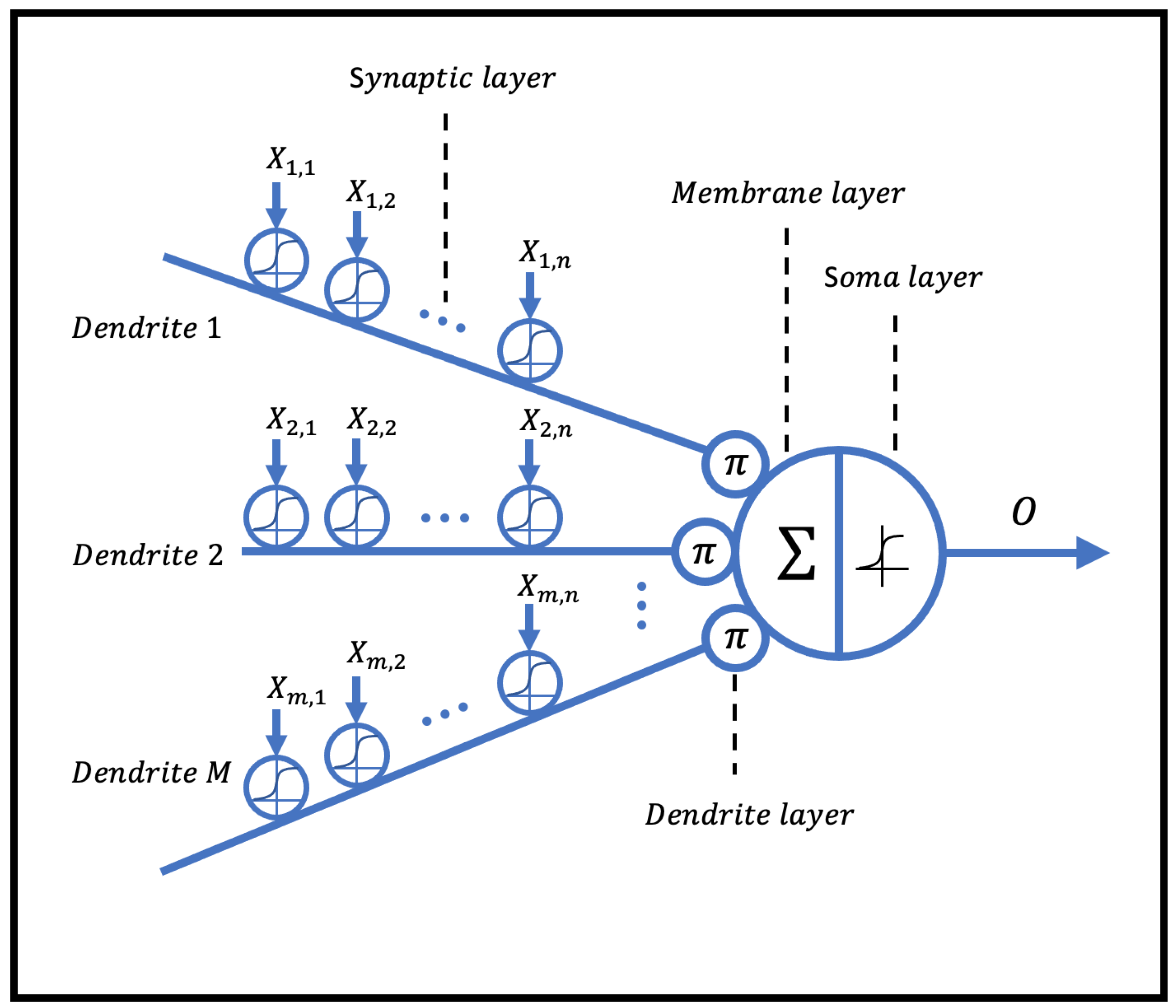
The dendritic neuron model consists of four main layers: the synaptic layer, dendritic layer, membrane layer, and soma layer, as illustrated in Figure 1. In this model, nonlinear computations are incorporated within a single dendritic neuron.
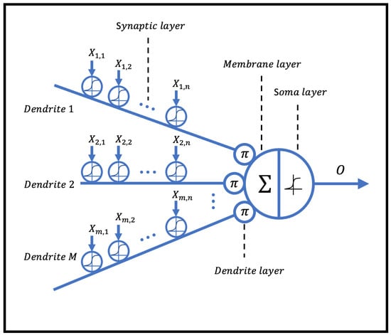
Figure 1.
The structure of the dendritic neural model.
2.1.1. Synaptic Layer
Synapses are structures that exist in the gaps between neurons. The dendritic neuron model receives input signals from the synaptic layer, which is expressed as follows:
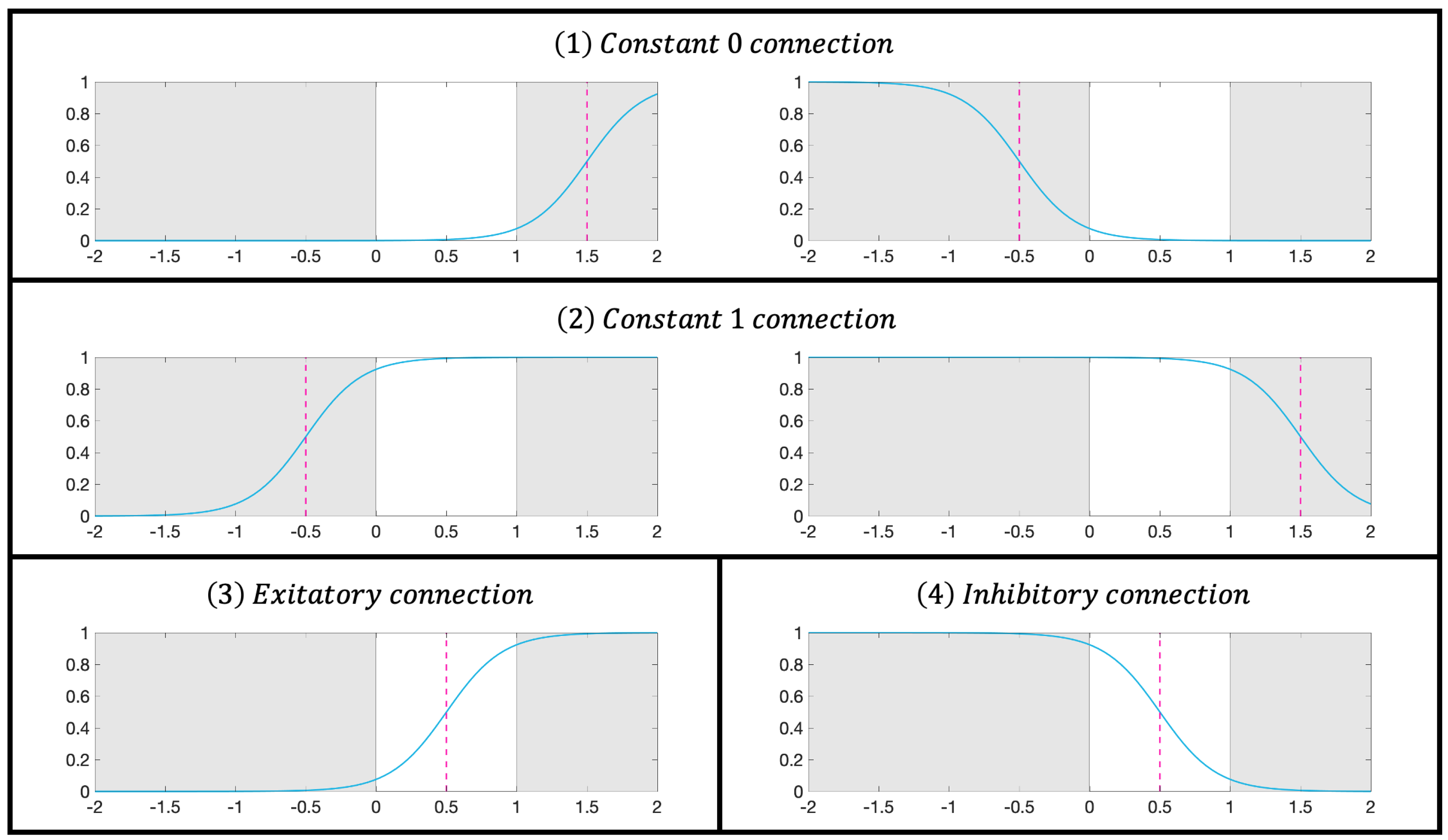
where k is a positive constant; denotes the input of the j-th synapse in the i-th synaptic layer; and are the weight and threshold, respectively; and S indicates the output of the corresponding synaptic position. Within the range of , there are four possible biomimetic connections—constant 0, constant 1, excitatory connection, and inhibitory connection—as shown in Figure 2.
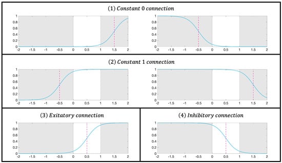
Figure 2.
Activation patterns in the synaptic layer.
2.1.2. Dendritic Layer
A dendritic layer receives multiple synaptic outputs and imparts nonlinear relationships to them. The expression is as follows:
where represents the output of the j-th dendritic layer.
2.1.3. Membrane Layer
The membrane layer performs linear summation on the output of the dendritic layer. The expression is as follows:
where M represents the output of the membrane layer.
2.1.4. Soma Layer
Similar to the synaptic layer, the soma layer utilizes the sigmoid function to simulate the excitatory and inhibitory outputs of neurons. The expression is as follows:
where is a constant. represents the activation threshold of the soma. O is the output of the soma, which also serves as the output of the dendritic neuron model.
2.2. Local Motion Direction Detection Neurons
In the proposed AVS, the complete retinal intermediate structures are utilized, including PCs, HCs, BCs, ACs, and DSGCs, along with their spatial structures and connectivity relationships. We sequentially model the relevant cells. Here, we consider DSGCs as local motion direction neurons (LMDNs) within AVS responsible for gathering local motion direction information.
2.2.1. Photoreceptor Cells
PCs are responsible for optoelectronic signal conversion. Here, we use 0 and 1 to represent the absence and presence of optical signals, respectively. The functionality of PCs is modeled using the following expression:
where i and j refer to the horizontal and vertical coordinates of pixels in the field of view, respectively, and t indicates time.
2.2.2. Bipolar Cells
BCs are considered to be sensitive to changes in light sources [13]. BCs are generally believed to be of three types: on BCs, off BCs, and on–off BCs. Due to their equivalence, we collectively refer to them as on–off BCs. The expressions are as follows:
where “” indicates that changes from 0 to 1 during a certain time interval, whereas “” represents changing from 1 to 0 during the time interval, and “” indicates that the light remains unchanged.
2.2.3. Horizontal Cells
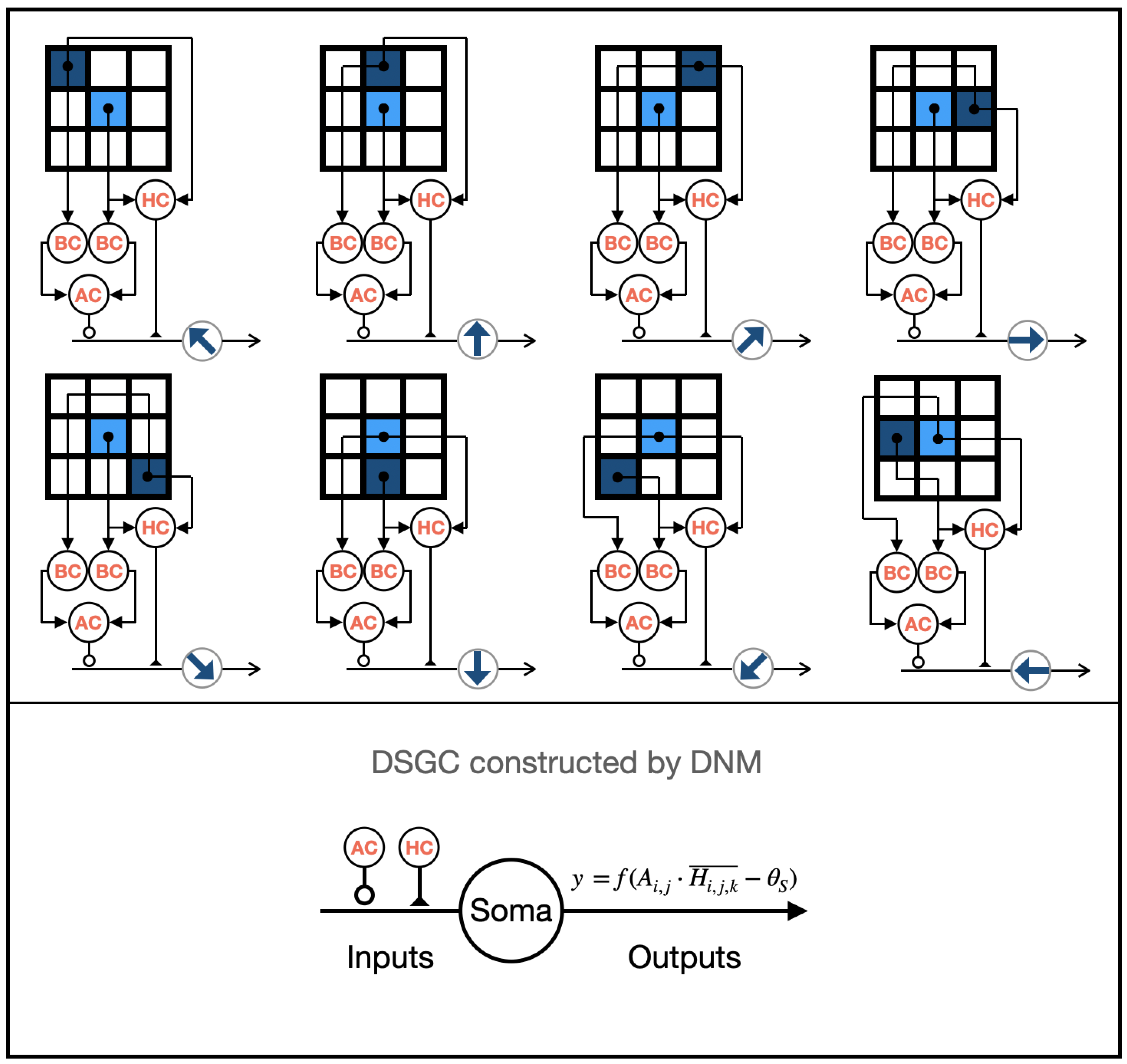
HCs are considered lateral modulators [12], simultaneously connecting to PCs and BCs in their terminals. The asymmetric structure is believed to be crucial for generating direction selectivity [3]. Additionally, in initial research, Barlow pointed out that HCs may play a critical role [10]. Based on this, we designed eight types of asymmetrically connected HCs, each involved in detecting different local motion directions, as shown in Figure 3. The functional expression of HCs is defined as follows:
where H represents the output of HCs, and k represents the types of directional preferences.
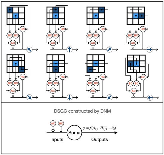
Figure 3.
The structure of the eight types of LMDNs.
2.2.4. Amacrine Cells
ACs are believed to be involved in the lateral modulation of directional selectivity in the back end of BCs [15]. They simultaneously connect to the synaptic layers of neighboring BCs and DSGCs [28]. We enable ACs to intercommunicate the functional response results of relevant sensitive direction neighborhoods in BCs, thereby guiding DSGCs with inputs from both local and neighboring BCs. The functional expression of ACs is defined as follows:
where and represent two boundary conditions in the neighborhood, and their positions are determined by the value of k.
2.2.5. Direction-Selective Ganglion Cells
DSGCs receive inputs from BCs and ACs at their dendritic terminals [29]. In the retina’s direction-selective pathway, HCs indirectly influence the output of BCs by affecting their inputs, thereby impacting the inputs of DSGCs [12]. ACs, on the other hand, indirectly affect the inputs of DSGCs by influencing the output of BCs [30]. Based on these principles, we modeled eight classes of DSGCs and their related direction-selective pathways using a dendritic neuron model, each sensitive to different motion directions, as shown in Figure 3. The functional expressions for the synaptic and dendritic layers of DSGCs are as follows:
where D refers to the output of DSGCs. The outputs of ACs and HCs are implemented using excitatory and inhibitory synapses in the dendritic neural model.
Since there is a dendritic layer in this model, the input to the membrane layer of DSGCs is the same as in the dendritic layer. The expressions of the membrane layer and soma layer of DSGCs are as follows:
where M and S represent the outputs of the membrane layer and the soma layer of DSGCs (LMDNs), respectively; denotes the threshold of the soma; and .
2.3. Global Scanning
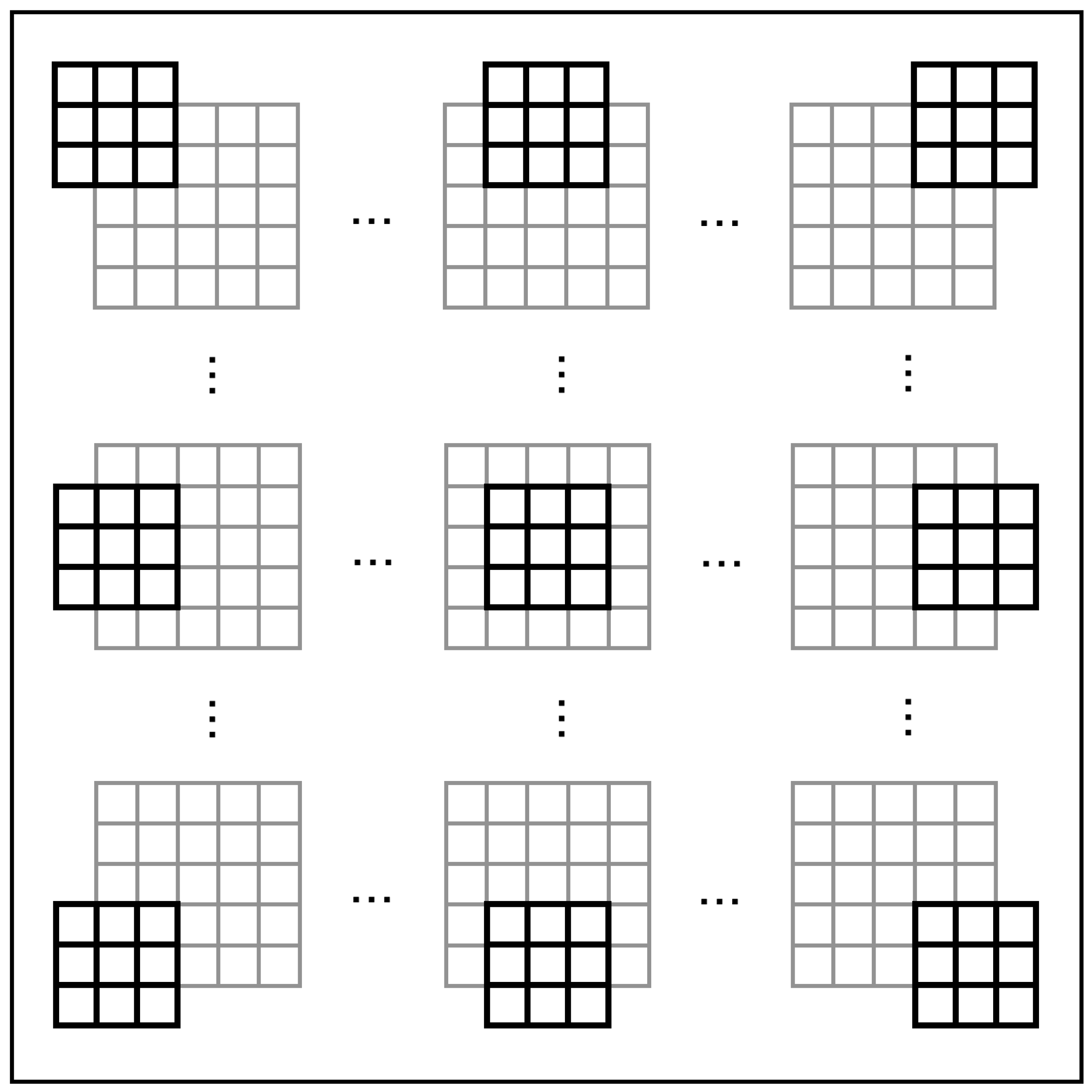
We utilize DSGCs to obtain local motion direction information from each visual field section in the retina, a process we refer to as “global scanning”. As shown in Figure 4, each DSGC acquires information from nine PCs within its local receptive field, processes it, and generates output. With these outputs, we employ a simple spiking neural network to process and derive the results of global motion direction detection.
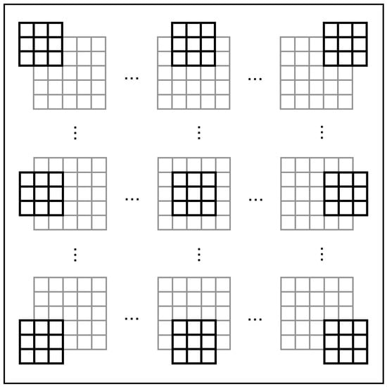
Figure 4.
The global scanning process by LMDNs.
2.4. Global Motion Direction Detection Neurons
We use a simple spiking neural network mechanism to acquire global motion direction information and propose a global motion direction detection neuron (GMDN) to elucidate how the cortex processes signals from the output of retinal direction-selective ganglion cells (DSGCs). In a visual area of , the functional expression of GMDNs is as follows:
where G represents the output of GMDNs.
2.5. The Mechanism of the Artificial Visual System
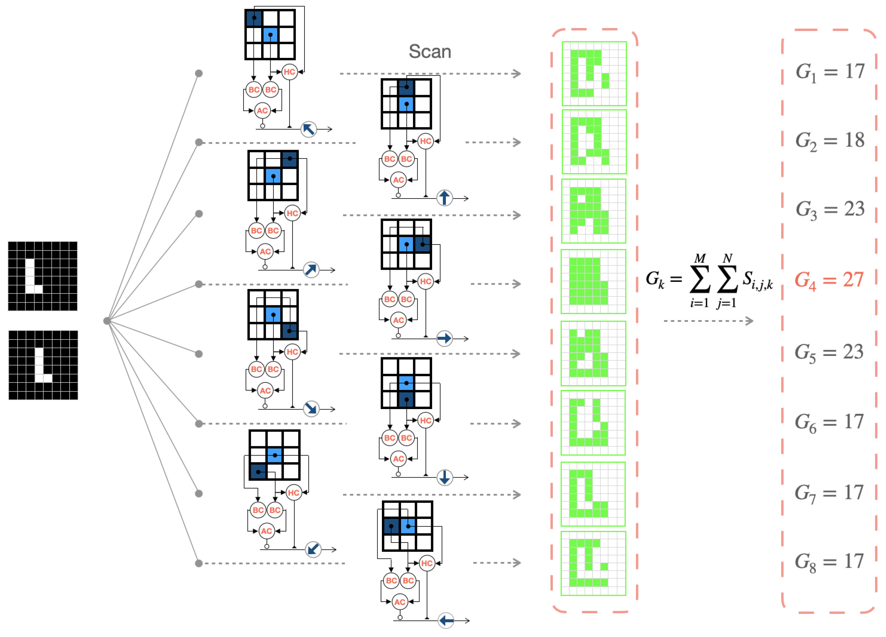
Here, we use an example of an object in the shape of an “L” moving to the right to describe the overall mechanism of AVS, as shown in Figure 5. In the case of a continuously moving object, consecutive frames are taken as input. The eight types of LMDNs (DSGCs) distributed across the retina scan each local region of the input images and output their respective feature maps (highlighted in green for activated regions). Finally, the corresponding GMDNs generate output spiking response intensities based on their respective feature maps. We infer the global motion direction from the direction of the strongest spiking response. In Figure 5, the right-sensitive GMDNs exhibit the highest spiking response intensity (27), successfully detecting the motion direction of the object in the field of view at that moment.
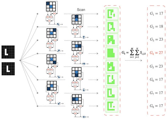
Figure 5.
The process of the artificial visual system for motion direction detection in color images.
3. Experiments
The experiment comprises four parts: effectiveness testing, efficiency testing, generalization performance testing, and other analyses.
3.1. Effectiveness Test
The effectiveness test is conducted based on one million sets of randomly generated binary object motion instances. Each instance is generated as follows. First, random shapes of objects are generated according to the given object pixel scale. Each pixel in the object is adjacent to any other pixel that constitutes the object. Secondly, the object is randomly placed on a background of a different binary value. Thirdly, the object undergoes continuous motion in any direction. Fourthly, any two consecutive frames are extracted from the continuous motion video to serve as inputs for AVS. In the experiment, we select ten sets of values (1, 2, 4, 8, 16, 32, 64, 128, 256, and 512) as the tested object sizes. Eight motion directions are uniformly assigned to each size of the tested object. The relevant instances in this experiment are described in subsequent sections.
In the effectiveness test, we found that AVS was able to complete all one million instances of object motion detection with 100% accuracy, with 12,500 instances of object motion for each of the 10 differently sized objects in all directions. The relevant results are shown in Table 1, where U, UR, R, LR, D, LL, L, and UL represent the eight motion directions, i.e., up, upper right, right, lower right, down, lower left, left, and upper left, respectively. This indicates that the proposed AVS not only effectively detects the direction of object motion but also exhibits a high level of efficiency.

Table 1.
The experimental results of the noiseless test on 10 sizes of objects.
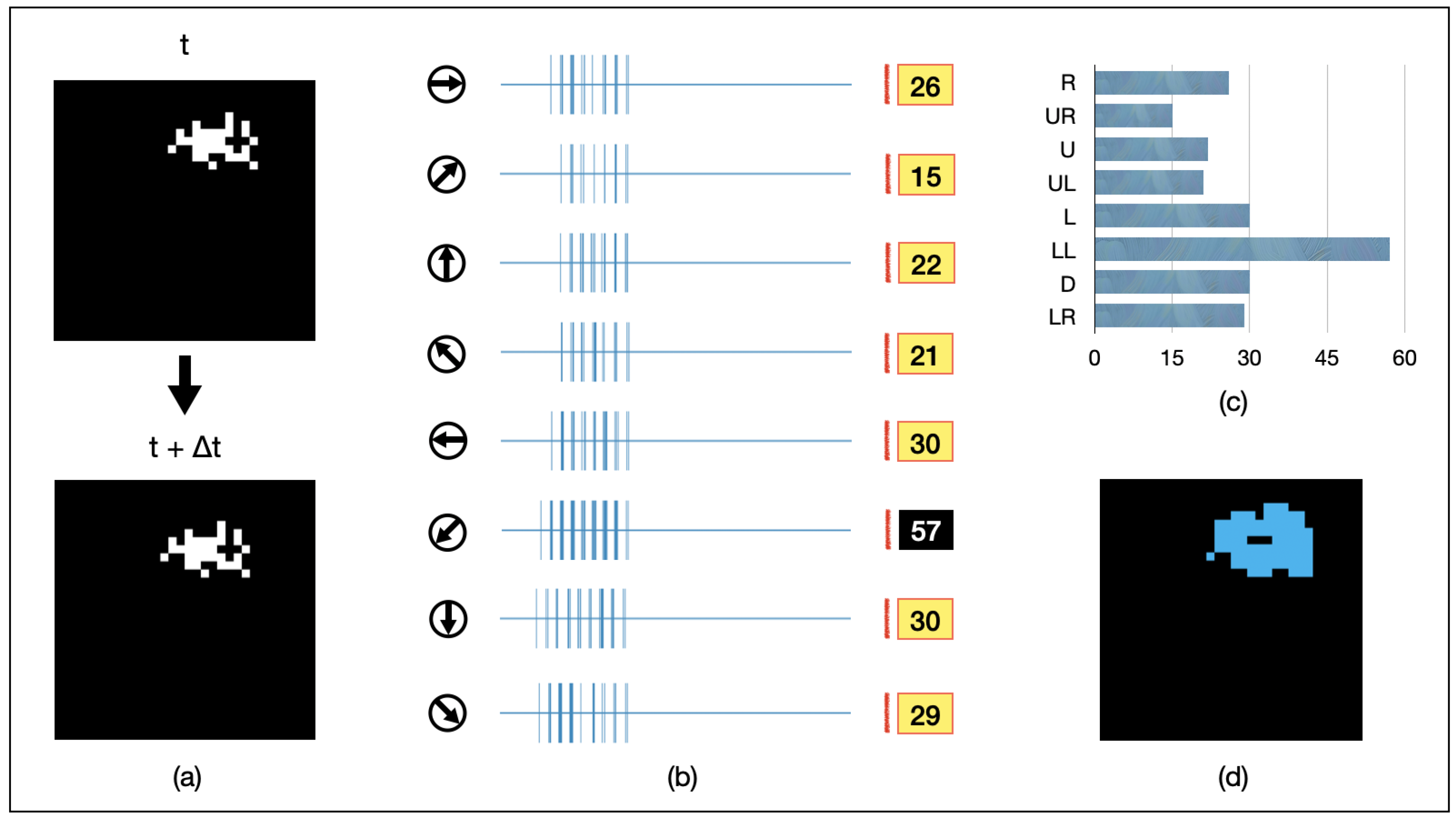
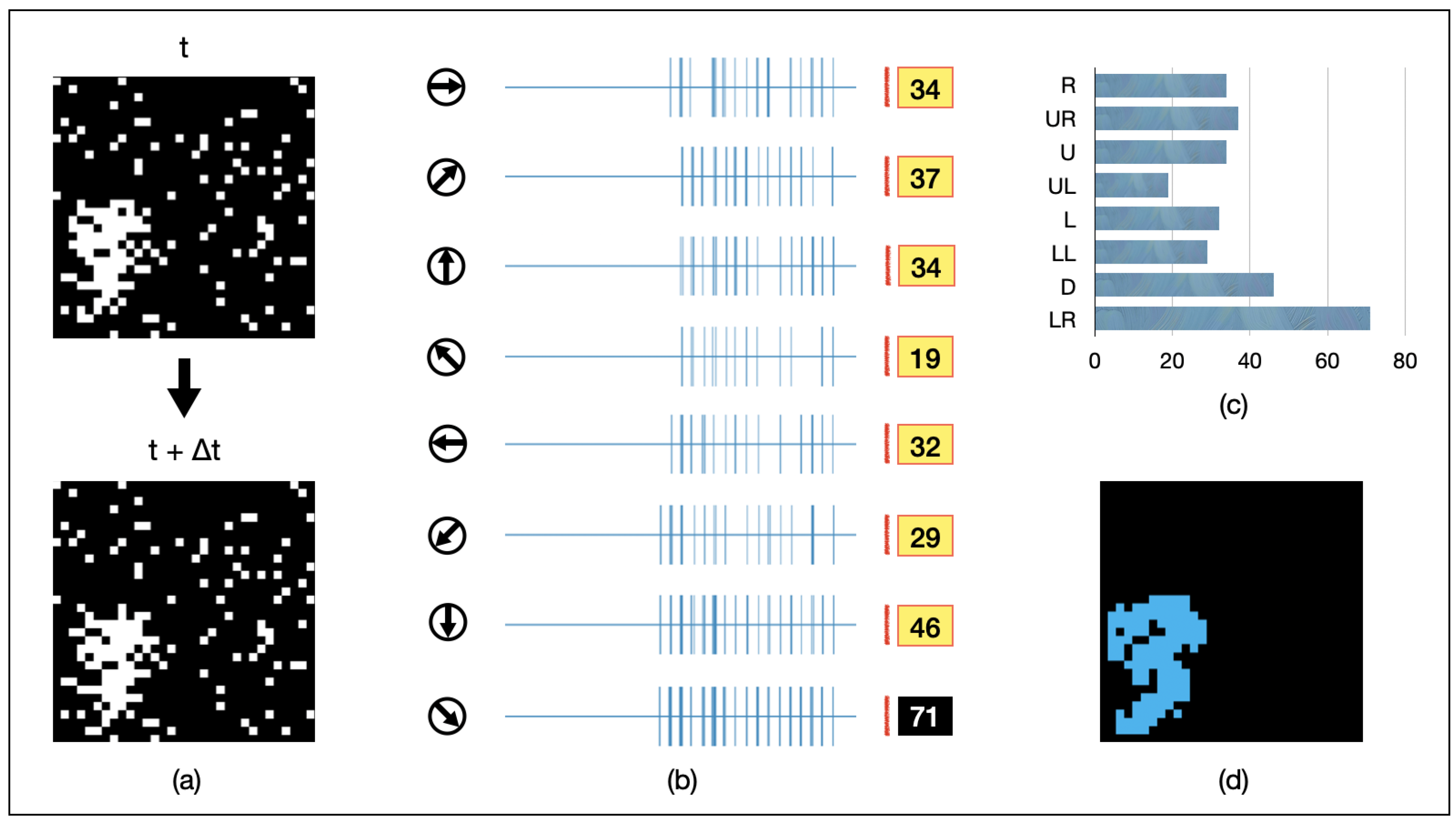
We present an example of AVS in Figure 6. A randomly shaped object of 16 pixels is continuously moving towards the lower-left direction. It is randomly captured in two adjacent frames, as depicted in Figure 6a. The spiking intensity responses of each GMDN after being fed into AVS are shown in Figure 6b, and the resulting histogram is presented in Figure 6c. Among them, GMDNs sensitive to the lower-left direction exhibit significantly stronger spiking responses (activated 57 times in total). As a result, AVS confidently detects the correct direction of object motion. Furthermore, the regions of activation for all eight groups of LMDNs are recorded in Figure 6d (in blue). This result demonstrates that AVS can effectively track the position of moving objects.

Figure 6.
An example for AVS detecting the motion direction of a 32-pixel object. (a) visualizes inputs of the example instance; (b) represents the activation map of LMDNs; (c) draws the corresponding histogram; (d) shows the regions activated by all the LMDNs.
3.2. Efficiency Test
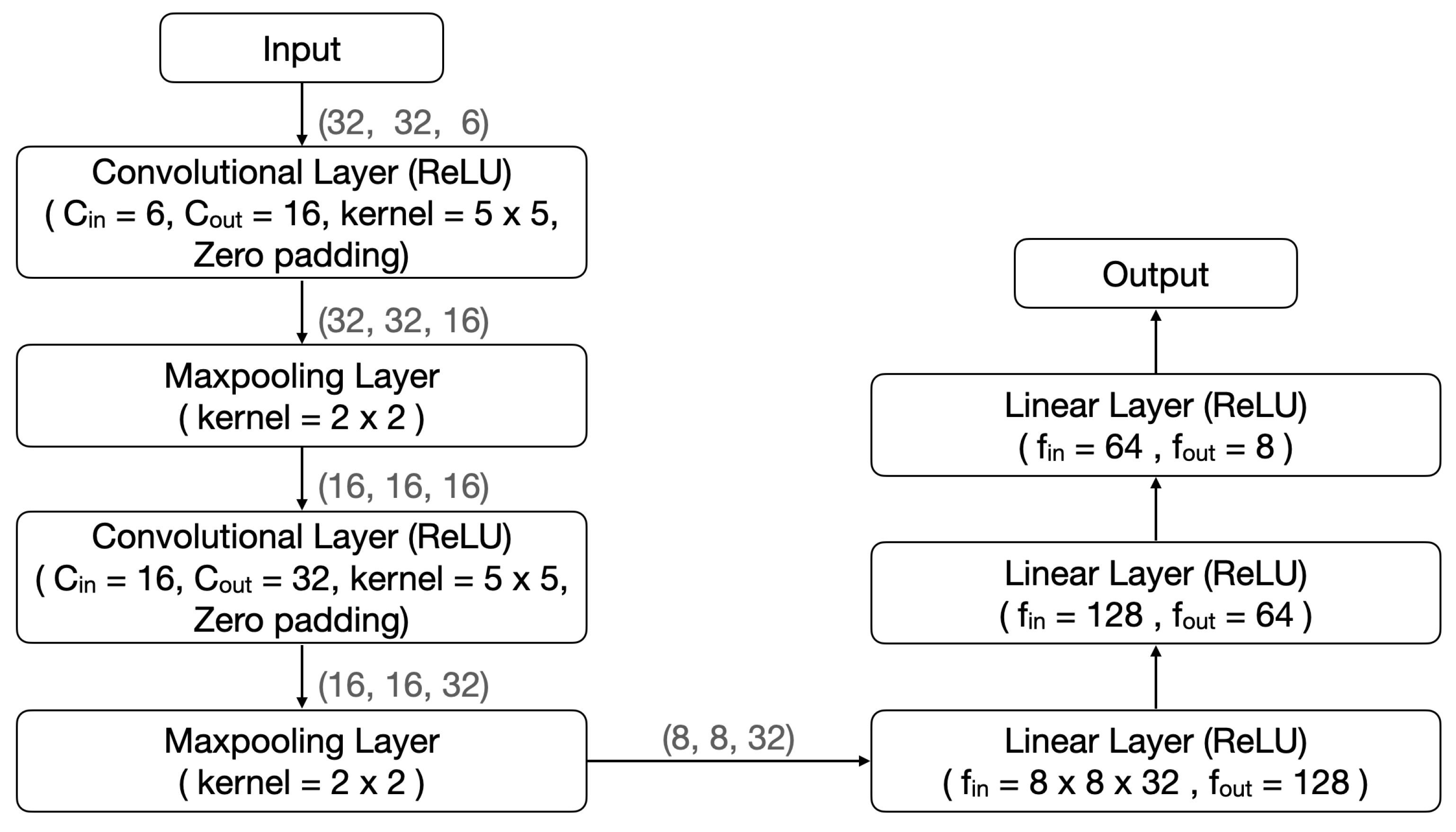
In view of the excellent performance of AVS in the effectiveness testing, we conducted a comparative test to assess its efficiency using two well-known CNNs. The two CNNs chosen for comparison are LeNet-5 [26] and EfficientNetB0 [27], both of which have made remarkable contributions to various image recognition tasks [31,32,33]. LeNet-5 and EfficientNetB0 are 7-layer and 18-layer deep networks, respectively. Their structures are shown in Figure 7 and Figure 8, respectively.

Figure 7.
The LeNet-5 structure in comparison with that of AVS.

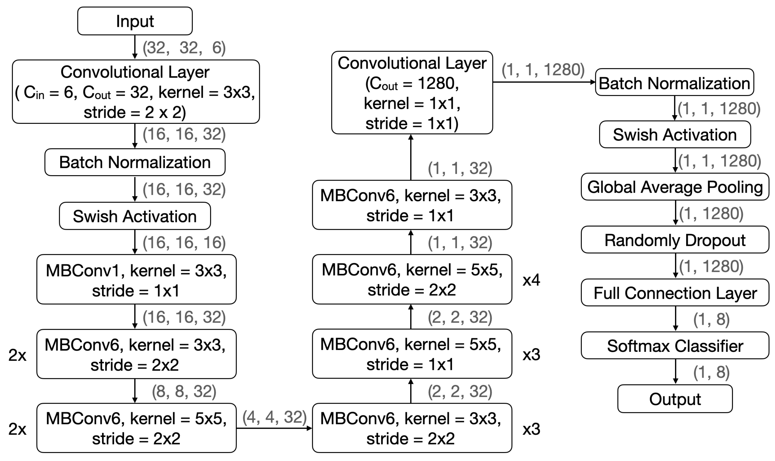
Figure 8.
The EfficientNetB0 structure in comparison with that of AVS.
During the experiments, one million instances were divided into training and testing sets in an 8:2 ratio. The learning process of CNNs involved 100 epochs with a learning rate of 0.001 using the Adam optimizer [34]. To minimize the impact of variations during the learning process, the experimental results were based on the average of 30 training runs (Table 2).
Table 2.
The comparison results between AVS and CNNs in detecting 10 sizes of objects.
3.3. Generalizability Test
Generalization is crucial for image recognition tasks. Studies have shown that although some neural network algorithms have approached or even surpassed human-level accuracy in certain image pattern recognition tasks, the generalization ability of human brain computation goes beyond what advanced deep learning algorithms can achieve [35,36]. For AVS, we designed two generalization tests to assess its generalization performance and brain-like features. Leveraging effective instance generation methods for effectiveness testing, we created two new test sets, each incorporating static and dynamic random noise.
3.3.1. Static Noise Test
We randomly select some pixels within the image scope and add static noise at those positions. The static noise remains unchanged over time. As shown in Figure 9a, a 64-pixel object is moving towards the lower-right corner of the field of view. Static noise is present around the object and in other areas as well. Upon receiving the input image, AVS outputs the spiking response intensities of GMDNs in different directions, as depicted in Figure 9b. From the spiking response histogram shown in Figure 9c, it can be observed that AVS exhibits the strongest response to the movement towards the lower-right direction, which aligns with the motion direction of the input object instance. As shown in Figure 9d, AVS effectively filters out the static noise. Even in a cluttered environment, AVS is capable of real-time tracking of the object’s motion position.
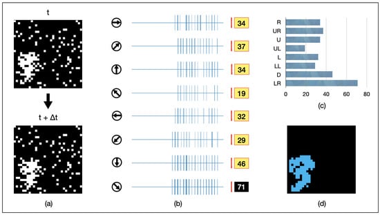
Figure 9.
An example of AVS detecting the motion direction of a 64-pixel object under random static noise. (a) visualizes inputs of the example instance; (b) represents the activation map of LMDNs; (c) draws the corresponding histogram; (d) shows the regions activated by all the LMDNs.
The static noise experiment was conducted under three different noise levels, as shown in Table 3. LeNet-5 failed to learn successfully, maintaining a very low recognition rate of 12.5% in various noise environments. AVS, in the presence of static noise, struggled to maintain high detection performance for small objects but retained a detection accuracy of over 90% for objects larger than 16 pixels. EfficientNet also experienced a noticeable decline in detection accuracy for objects of all sizes. Even for the largest 512-pixel objects, it exhibited a detection accuracy of less than 70% under 10% noise capacity. These results suggest that while static noise does affect the detection accuracy of AVS, its impact is significantly smaller compared to that of CNNs.
Table 3.
The comparison results between AVS and CNNs for 64-pixel object motion direction detection within static noise.
3.3.2. Dynamic Noise Test
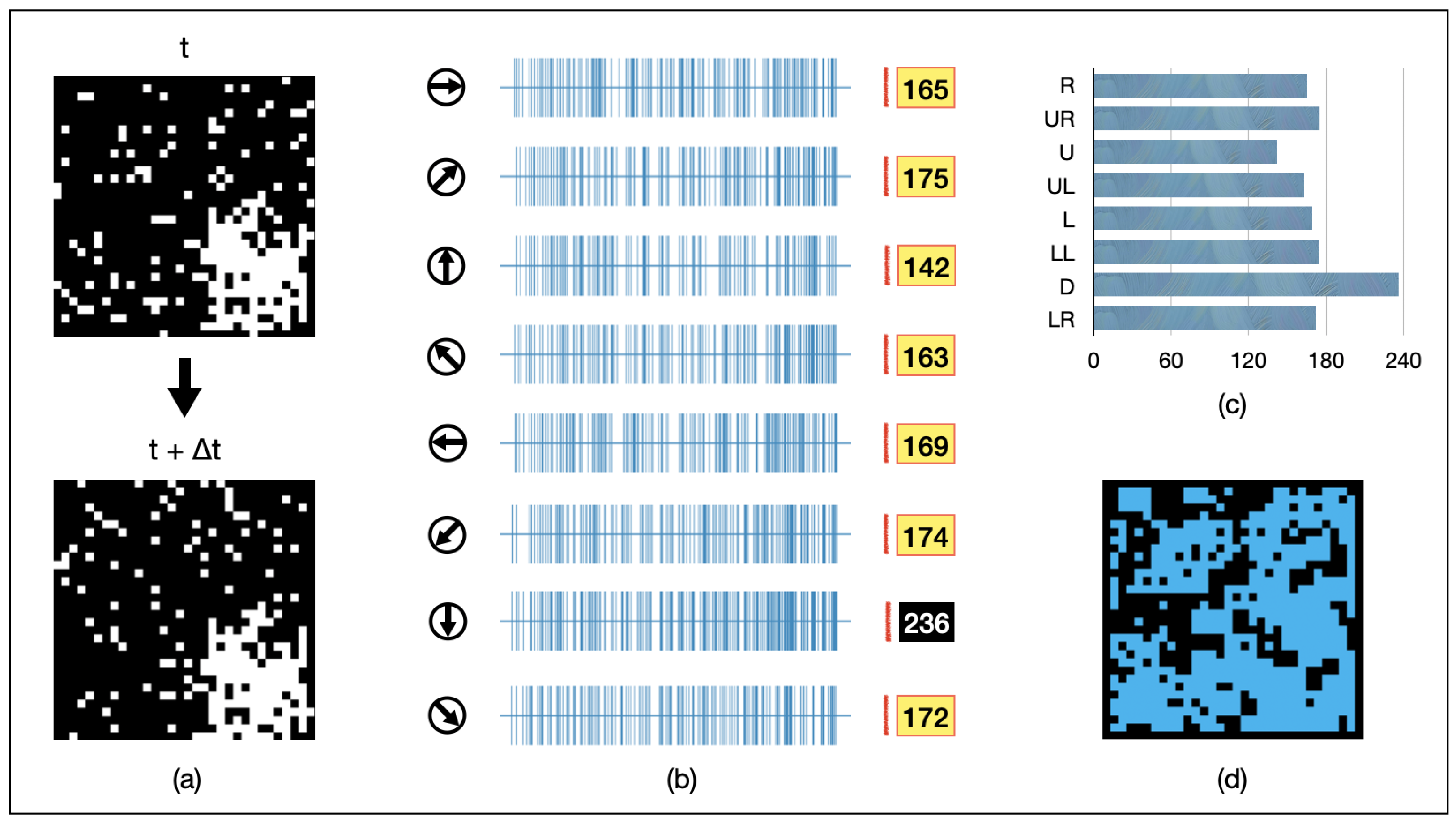
We selected some pixels within the image range, added noise to these positions, and made their locations change randomly over time. An example under this dynamic noise is shown in Figure 10a. In the bottom-right corner of the field of view, there is a 128-pixel object moving downward. At different moments, the noise points vary randomly in the image. The spiking intensity of GMDNs is shown in Figure 10b,c. The spiking response intensity of the GMDNs in the downward direction is higher than in other directions, allowing AVS to correctly detect the direction of the object’s movement in this instance. However, all activated LMDN points failed to track the object exactly, as depicted in Figure 10d. This is because the changing positions of the noise caused extensive activation of LMDNs.
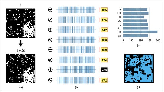
Figure 10.
An example of AVS in detecting the motion direction of a 128-pixel object under random dynamic noise. (a) visualizes inputs of the example instance; (b) represents the activation map of LMDNs; (c) draws the corresponding histogram; (d) shows the regions activated by all the LMDNs.
The dynamic noise experiment was conducted under three different noise levels, as shown in Table 4. LeNet-5 exhibited a 12.5% failure rate in detection due to unsuccessful learning. Both AVS and EfficientNet experienced a further decline in detection accuracy in the presence of static noise. However, in comparison to EfficientNet, AVS still demonstrates a clear performance advantage. For objects with pixel dimensions greater than 128, AVS achieved a detection accuracy of over 90% across all three noise levels. EfficientNet, on the other hand, showed its highest detection accuracy of 62.02% for 512-pixel objects under 10% noise capacity.
Table 4.
The comparison results between AVS and CNNs for 128-pixel object motion direction detection under dynamic noise.
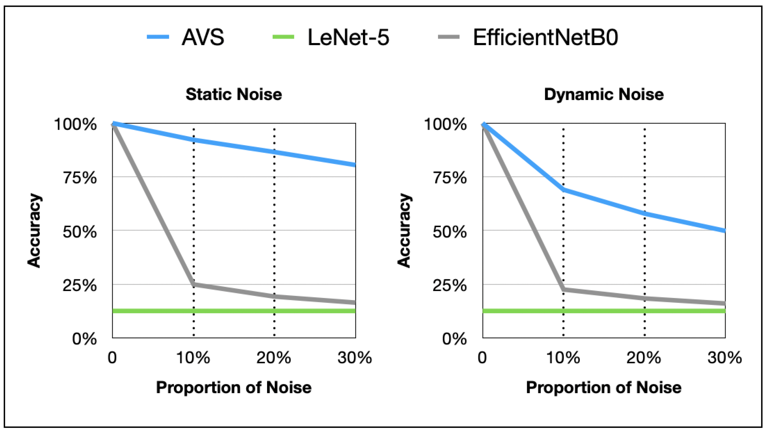
3.3.3. Anti-Noise Plot Analysis
The line graphs of noise resistance performance of AVS and two classical CNNs on differently sized objects in the two noise tests are shown in Figure 11. AVS outperforms CNNs significantly in terms of effectiveness, generalization, and noise resistance. The impact of dynamic noise on AVS and CNNs is notably stronger than that of static noise.
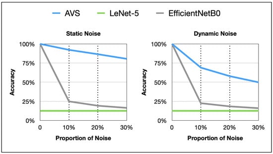
Figure 11.
Plot comparison between AVS and CNNs in detecting object motion direction under two noise types.
3.4. Summary of Comparison between AVS and CNNs
The other characteristics of AVS observed during the experiment are summarized in Table 5. First, based on explicit knowledge from neuroscience, AVS can be deployed and perform neurocomputational functions without the need for learning. Second, compared to deep learning algorithms, AVS exhibits specificity in solving motion direction selection, as it directly models human brain-related visual neural pathways. Third, AVS does not involve any hyperparameters or learning parameters, presenting a concise and well-defined hierarchical structure. Consequently, compared to mainstream image recognition algorithms, AVS is highly amenable to hardware implementation. Fourth, owing to its clear neuroscientific foundation, AVS possesses biologically inspired characteristics such as high interpretability and generalizability. This openness contributes to promising real-world applications of AVS. In comparison to CNNs, AVS’s biological nature appears to endow it with superior effectiveness and adaptability when addressing relevant problems. Additionally, AVS’s biomimetic advantages may provide inspiration and insights for the advancement of existing state-of-the-art neural network algorithms.
Table 5.
Other comparisons between AVS and CNNs.
3.5. Discussions
Here, we engage in further comprehension and discussion concerning AVS.
3.5.1. Expanding Detection in Multiple Directions
For simplicity, the AVS proposed in this article only includes eight fundamental directions. However, if we wish to detect more motion directions, it is only necessary to expand the LMDNs’ receptive field. For instance, the current receptive field corresponds to 8 directions, the corresponds to 16 directions, and the corresponds to 24 directions.
3.5.2. Application Expansion of Global Motion Direction
In the first part of the AVS, we successfully quantified and implemented the relevant pathways of DSGCs, which are used to extract local motion direction information. In the latter part of AVS, we explained the integration of motion direction information from local to global using a spiking computation mechanism. Global motion direction refers to the most apparent motion direction occurring in an animal’s visual field of view. However, this information has not undergone further processing in the brain, i.e., rational (or intelligent) processing. Therefore, although AVS comprehensively and effectively explains the mechanisms for extracting primary motion direction information before reaching the cortex and could be applied in some practical detection scenarios, there is still room to improve the flexibility of AVS as an algorithm. For example, it is important to determine how to enable AVS to recognize the motion direction of objects within specific local regions in the field of view. We suggest utilizing existing neural network algorithms to track and frame specific areas, allowing AVS to collect global motion direction information from those regions, achieving a flexible and efficient application.
3.5.3. Development into a Learning Model
The plasticity of neural synapses [37,38] prompts us to consider the possibility of a learnable AVS. The existing AVS functional architecture can be restructured into a trainable AVS. This can be achieved by either learning the parameters through random initialization or using the specific architecture presented in this paper as the initializer for the optimization and learning process.
3.5.4. Orientation, Velocity, and Universal Framework in Three-Dimensional Scenes
Some studies have suggested that the positional information in the shape of objects is also partially inherited from DSGCs [39]. Therefore, the approach presented in this paper contributes to the understanding of the principles of orientation selection. Moreover, the velocity characteristics are theoretically derived from the direction-selective properties. In conclusion, the framework proposed in this paper provides insights and references for object shape orientation, motion direction, and motion speed in both two-dimensional and three-dimensional scenes.
3.5.5. Foundation for the Development Future Novel Neural Network Algorithms
The existing AVS is inspired by the front end of the brain’s visual system, which is used to extract the most fundamental visual information. Through extensive comparisons, we validated the various advantages of AVS for neural network algorithms. In the future, AVS may contribute to feature pre-extraction in neural network algorithms. The adaptable AVS can also be embedded within neural network algorithms to obtain a more tightly integrated novel neural network algorithm.
3.5.6. Advantages and Potential Challenges in Future Development
The implementation of AVS in the field of engineering comes with a clear advantage: biological interpretability. While current neural network algorithms excel in handling engineering problems, their lack of interpretability imposes limitations on their comprehensive application in certain domains involving critical ethical concerns, such as the medical industry. AVS has the potential to offer a dual advantage to existing neural network algorithms in terms of interpretability and specific functionality. Furthermore, research on AVS could inspire additional related studies exploring the specific potential of modeling the biological nervous system, gradually advancing the interpretability and universality of neural network algorithms from a new perspective. However, it should be noted that due to its reliance on retinal direction-selective pathways, AVS for motion direction detection remains a specific algorithm for addressing motion direction detection issues. In future development, whether through embedded integration or fundamental upgrades, attention should be paid to addressing and rectifying the universality limitations of AVS.
4. Conclusions
In this paper, we leveraged knowledge from neuroscience about motion direction extraction pathways in mammalian retinas. We modeled the specific functions of each component cell and proposed a comprehensive motion direction detection and interpretation mechanism from photoreceptors to the cortex called AVS. By testing for effectiveness, efficiency, and generalization, we verified that this interpretation mechanism exhibits outstanding biomimetic performance. Compared to state-of-the-art deep learning algorithms, AVS demonstrates higher accuracy, robust generalization ability, concise structure, strong biomimicry, high interpretability, and hardware advantages. While providing a motion direction detection mechanism for 2D inputs, AVS also unprecedentedly quantitatively explains the neural computational mechanism of retinal direction-selective pathways. By developing a novel brain-inspired feature extraction algorithm, we encourage neuroscientists to pay attention to and further explore the computational principles of relevant neural pathways. Looking ahead, the organic integration of AVS with deep learning algorithms should be thoroughly considered, while simultaneously delving into the specific principles and mechanisms of related neural computation.
Author Contributions
Conceptualization, S.T., Z.T. and Y.T.; methodology, S.T., Z.T. and Y.T.; software, S.T., X.Z., Y.H. and Y.T.; visualization, S.T., X.Z. and Y.H.; writing—original draft, S.T.; writing—review and editing, S.T., Z.T. and Y.T.; supervision, Z.T. and Y.T.; project administration, Z.T. All authors have read and agreed to the published version of the manuscript.
Funding
This research was partially supported by the Japan Society for the Promotion of Science (JSPS) KAKENHI under grant JP22H03643 and the Japan Science and Technology Agency (JST) through the Establishment of University Fellowships towards the Creation of Science Technology Innovation under grant JPMJFS2115.
Data Availability Statement
The source code are available at https://github.com/terrysc/completely-modeled-AVS (accessed on 23 August 2023).
Conflicts of Interest
The authors declare no conflict of interest.
References
- Baden, T.; Euler, T.; Berens, P. Understanding the retinal basis of vision across species. Nat. Rev. Neurosci. 2020, 21, 5–20. [Google Scholar] [CrossRef] [PubMed]
- Vlasits, A.L.; Euler, T.; Franke, K. Function first: Classifying cell types and circuits of the retina. Curr. Opin. Neurobiol. 2019, 56, 8–15. [Google Scholar] [CrossRef] [PubMed]
- Vaney, D.I.; Sivyer, B.; Taylor, W.R. Direction selectivity in the retina: Symmetry and asymmetry in structure and function. Nat. Rev. Neurosci. 2012, 13, 194–208. [Google Scholar] [CrossRef] [PubMed]
- Rasmussen, R.; Yonehara, K. Contributions of retinal direction selectivity to central visual processing. Curr. Biol. 2020, 30, R897–R903. [Google Scholar] [CrossRef]
- Kerschensteiner, D. Feature detection by retinal ganglion cells. Annu. Rev. Vis. Sci. 2022, 8, 135–169. [Google Scholar] [CrossRef] [PubMed]
- Barlow, H.B.; Hill, R.M. Selective sensitivity to direction of movement in ganglion cells of the rabbit retina. Science 1963, 139, 412–414. [Google Scholar] [CrossRef] [PubMed]
- Hoon, M.; Okawa, H.; Della Santina, L.; Wong, R.O. Functional architecture of the retina: Development and disease. Prog. Retin. Eye Res. 2014, 42, 44–84. [Google Scholar] [CrossRef]
- Mauss, A.S.; Vlasits, A.; Borst, A.; Feller, M. Visual circuits for direction selectivity. Annu. Rev. Neurosci. 2017, 40, 211–230. [Google Scholar] [CrossRef]
- Hassenstein, B.; Reichardt, W. Systemtheoretische analyse der zeit-, reihenfolgen-und vorzeichenauswertung bei der bewegungsperzeption des rüsselkäfers chlorophanus. Z. Naturforschung B 1956, 11, 513–524. [Google Scholar] [CrossRef]
- Barlow, H.; Levick, W.R. The mechanism of directionally selective units in rabbit’s retina. J. Physiol. 1965, 178, 477. [Google Scholar] [CrossRef]
- Burns, M.E.; Baylor, D.A. Activation, deactivation, and adaptation in vertebrate photoreceptor cells. Annu. Rev. Neurosci. 2001, 24, 779–805. [Google Scholar] [CrossRef]
- Chapot, C.A.; Euler, T.; Schubert, T. How do horizontal cells ‘talk’to cone photoreceptors? Different levels of complexity at the cone–horizontal cell synapse. J. Physiol. 2017, 595, 5495–5506. [Google Scholar] [CrossRef] [PubMed]
- Euler, T.; Haverkamp, S.; Schubert, T.; Baden, T. Retinal bipolar cells: Elementary building blocks of vision. Nat. Rev. Neurosci. 2014, 15, 507–519. [Google Scholar] [CrossRef] [PubMed]
- Masland, R.H. The tasks of amacrine cells. Vis. Neurosci. 2012, 29, 3–9. [Google Scholar] [CrossRef] [PubMed]
- Taylor, W.; Smith, R. The role of starburst amacrine cells in visual signal processing. Vis. Neurosci. 2012, 29, 73–81. [Google Scholar] [CrossRef]
- Sanes, J.R.; Masland, R.H. The types of retinal ganglion cells: Current status and implications for neuronal classification. Annu. Rev. Neurosci. 2015, 38, 221–246. [Google Scholar] [CrossRef]
- Cruz-Martín, A.; El-Danaf, R.N.; Osakada, F.; Sriram, B.; Dhande, O.S.; Nguyen, P.L.; Callaway, E.M.; Ghosh, A.; Huberman, A.D. A dedicated circuit links direction-selective retinal ganglion cells to the primary visual cortex. Nature 2014, 507, 358–361. [Google Scholar] [CrossRef]
- Han, M.; Todo, Y.; Tang, Z. Mechanism of motion direction detection based on barlow’s retina inhibitory scheme in direction-selective ganglion cells. Electronics 2021, 10, 1663. [Google Scholar] [CrossRef]
- Tao, S.; Todo, Y.; Tang, Z.; Li, B.; Zhang, Z.; Inoue, R. A novel artificial visual system for motion direction detection in grayscale images. Mathematics 2022, 10, 2975. [Google Scholar] [CrossRef]
- Gallego, A. Horizontal and amacrine cells in the mammal’s retina. Vis. Res. 1971, 11, 33-IN24. [Google Scholar] [CrossRef]
- Yoshida, K.; Watanabe, D.; Ishikane, H.; Tachibana, M.; Pastan, I.; Nakanishi, S. A key role of starburst amacrine cells in originating retinal directional selectivity and optokinetic eye movement. Neuron 2001, 30, 771–780. [Google Scholar] [CrossRef]
- Todo, Y.; Tamura, H.; Yamashita, K.; Tang, Z. Unsupervised learnable neuron model with nonlinear interaction on dendrites. Neural Netw. 2014, 60, 96–103. [Google Scholar] [CrossRef]
- Todo, Y.; Tang, Z.; Todo, H.; Ji, J.; Yamashita, K. Neurons with multiplicative interactions of nonlinear synapses. Int. J. Neural Syst. 2019, 29, 1950012. [Google Scholar] [CrossRef]
- Lindsay, G.W. Convolutional neural networks as a model of the visual system: Past, present, and future. J. Cogn. Neurosci. 2021, 33, 2017–2031. [Google Scholar] [CrossRef]
- Gupta, J.; Pathak, S.; Kumar, G. Deep learning (CNN) and transfer learning: A review. J. Phys. Conf. Ser. 2022, 2273, 12029. [Google Scholar] [CrossRef]
- LeCun, Y.; Bottou, L.; Bengio, Y.; Haffner, P. Gradient-based learning applied to document recognition. Proc. IEEE 1998, 86, 2278–2324. [Google Scholar] [CrossRef]
- Tan, M.; Le, Q. Efficientnet: Rethinking model scaling for convolutional neural networks. In Proceedings of the International Conference on Machine Learning, Long Beach, CA, USA, 10–15 June 2019; pp. 6105–6114. [Google Scholar]
- Taylor, W.R.; He, S.; Levick, W.R.; Vaney, D.I. Dendritic computation of direction selectivity by retinal ganglion cells. Science 2000, 289, 2347–2350. [Google Scholar] [CrossRef]
- Jain, V.; Murphy-Baum, B.L.; deRosenroll, G.; Sethuramanujam, S.; Delsey, M.; Delaney, K.R.; Awatramani, G.B. The functional organization of excitation and inhibition in the dendrites of mouse direction-selective ganglion cells. Elife 2020, 9, e52949. [Google Scholar] [CrossRef]
- Mills, S.L.; Massey, S.C. Differential properties of two gap junctional pathways made by AII amacrine cells. Nature 1995, 377, 734–737. [Google Scholar] [CrossRef]
- Forsyth, D.A.; Mundy, J.L.; di Gesú, V.; Cipolla, R.; LeCun, Y.; Haffner, P.; Bottou, L.; Bengio, Y. Object recognition with gradient-based learning. In Shape, Contour and Grouping in Computer Vision; Springer: Berlin/Heidelberg, Germany, 1999; pp. 319–345. [Google Scholar]
- Ma, D.Y. Summary of Research on Application of Deep Learning in Image Recognition. Highlights Sci. Eng. Technol. 2022, 1, 72–77. [Google Scholar] [CrossRef]
- Dhillon, A.; Verma, G.K. Convolutional neural network: A review of models, methodologies and applications to object detection. Prog. Artif. Intell. 2020, 9, 85–112. [Google Scholar]
- Kingma, D.P.; Ba, J. Adam: A method for stochastic optimization. arXiv 2014, arXiv:1412.6980. [Google Scholar]
- Szegedy, C.; Zaremba, W.; Sutskever, I.; Bruna, J.; Erhan, D.; Goodfellow, I.; Fergus, R. Intriguing properties of neural networks. arXiv 2013, arXiv:1312.6199. [Google Scholar]
- Nguyen, A.; Yosinski, J.; Clune, J. Deep neural networks are easily fooled: High confidence predictions for unrecognizable images. In Proceedings of the IEEE Conference on Computer Vision and Pattern Recognition, Boston, MA, USA, 7–12 June 2015; pp. 427–436. [Google Scholar]
- Holtmaat, A.; Svoboda, K. Experience-dependent structural synaptic plasticity in the mammalian brain. Nat. Rev. Neurosci. 2009, 10, 647–658. [Google Scholar]
- Legenstein, R.; Maass, W. Branch-specific plasticity enables self-organization of nonlinear computation in single neurons. J. Neurosci. 2011, 31, 10787–10802. [Google Scholar] [CrossRef]
- Ohki, K.; Chung, S.; Ch’ng, Y.H.; Kara, P.; Reid, R.C. Functional imaging with cellular resolution reveals precise micro-architecture in visual cortex. Nature 2005, 433, 597–603. [Google Scholar]
Disclaimer/Publisher’s Note: The statements, opinions and data contained in all publications are solely those of the individual author(s) and contributor(s) and not of MDPI and/or the editor(s). MDPI and/or the editor(s) disclaim responsibility for any injury to people or property resulting from any ideas, methods, instructions or products referred to in the content. |
© 2023 by the authors. Licensee MDPI, Basel, Switzerland. This article is an open access article distributed under the terms and conditions of the Creative Commons Attribution (CC BY) license (https://creativecommons.org/licenses/by/4.0/).