Nonlinear Dynamic Model-Based Position Control Parameter Optimization Method of Planar Switched Reluctance Motors

Abstract

Currently, there are few systematic position control parameter optimization methods for planar switched reluctance motors (PSRMs); how to effectively optimize the control parameters of PSRMs is one of the critical issues that needs to be urgently solved. Therefore, a nonlinear dynamic model-based position control parameter optimization method of PSRMs is proposed in this paper. First, to improve the accuracy of the motor dynamics model, a Hammerstein–Wiener model based on the BP neural network input–output nonlinear module is established by combining the linear model and nonlinear model structures so that the nonlinear and linear characteristics of the system are characterized simultaneously. Then, a position control parameter optimization system of PSRMs is developed using the established Hammerstein–Wiener model. In addition, with a self-designed simulated annealing adaptive particle swarm optimization algorithm (SAAPSO), the position control parameter optimization system is performed offline iteratively to obtain the optimal position control parameters. Simulations and experiments are carried out and the corresponding results show that the optimal position control parameters obtained by the proposed method can be directly applied in the actual control system of PSRMs and the control performance is improved effectively using the obtained optimal control parameters.

1. Introduction

The planar switched reluctance motor (PSRM) operating on the minimum reluctance principle is a kind of direct-drive planar motor. The motor features the advantages of simple structure, low cost, convenient installation, and high adaptability to extreme environments, such as high temperatures. As a result, the PSRMs show a promising candidate in precision positioning applications [1,2]. In 1988, the concept of a linear switched reluctance motor was first introduced in [3] and a prototype was successfully developed. Subsequently, in [4], the first generation of the PSRM prototype without the traditional mechanical transmission device was developed and a relevant control strategy was implemented on the prototype. Additionally, considerable progress has been made in several areas, including structural design and optimization, electromagnetic characteristics and iron consumption analysis, modeling, and position control [5,6,7]. Although much progress has been made for the PSRMs, the research on a systematic position control parameter optimization method has been scarcely reported. The selection of position control parameters is a critical task to achieve the excellent motion performance of PSRMs, since the position control parameters directly influence the performance of the position control of PSRMs system. Hence, this aspect is in urgent demand for further attention and investigation.

The position control parameters of PSRMs are mainly determined using empirical methods, which often fail to achieve optimal control performance. An example is [8]; the position control parameters are obtained by traversing the stable region of parameters. This approach can yield some applicable parameters for the position controller; however, it has limitations in terms of efficiency and there is no guarantee of achieving optimal parameters. Another example is [9]; the system control parameters are selected based on experience to ensure system stability; however, this method lacks a systematic approach to standardize the tuning process. In addition, the offline optimization method is attractive for obtaining the optimal position control parameter of PSRMs [10,11].

The premise of the offline optimization method for optimizing position control parameters is establishing an accurate motor system model [12]. Currently, the motor is usually modeled by applying the mechanism analysis method which results in a simplistic representation. However, the simplified model ignores some essential elements, such as unmodelled nonlinear friction force, disturbances, and time-varying parameters, thus failing to reflect the actual characteristics of the motor accurately. Hence, this modeling method has certain limitations and negatively impacts the control performance of the motor system [13]. To more accurately describe the PSRMs, there is an urgent demand to establish an accurate and effective modeling method for PSRMs. Doing so can provide valid system dynamic behaviors for parameter optimization and significantly improve the position control of the PSRM system.

The PSRM system inherently exhibits nonlinearity; thus, it is more effective to adopt a nonlinear model to describe the dynamic behaviors of the system [14,15]. As an emerging practical nonlinear modeling approach, the modular, nonlinear, and modeling method, which combines the characteristics of both linear and nonlinear model structures, is promising for PSRMs. This method represents the system by connecting nonlinear and linear links, treating them as independent modules constituting the overall nonlinear system [16,17]. Two widely applied models of the modular, nonlinear, and modeling method are the Hammerstein and the Wiener models. These two models are preferred due to their simple internal structure and efficient modeling capabilities. To further enhance the modeling ability, the Hammerstein–Wiener model is developed by combining the strengths of Hammerstein and the Wiener models [18,19,20,21,22]. In addition, the Hammerstein–Wiener model can incorporate a backpropagation (BP) neural network as a nonlinear module because of its strong learning capabilities and efficient nonlinear fitting ability [23,24,25,26]. By utilizing this combination of the Hammerstein–Wiener model and the BP neural network, the Hammerstein–Wiener model may significantly improve its overall modeling capabilities, mainly when dealing with the inherent nonlinearity of the motor system.

Based on the established nonlinear model, it is necessary to adopt an efficient and reliable optimization algorithm to optimize the position control parameters. In complex systems like PSRMs, the intelligent optimization algorithm has proven to be highly effective in its strong searching ability compared with the analytic method and the frequency domain method [27,28,29,30]. Among intelligent optimization algorithms, particle swarm optimization (PSO) has prominent advantages in convergence speed, initially proposed by Kennedy and Eberhart in 1995 as a swarm-intelligence-based optimization technology. In PSO, the optimization particles imitate the collective predation process of birds and allow for parallel and robust calculation processes [31,32,33]. This characteristic enhances the ability to find globally optimal solutions, giving it a computational advantage in analyzing various problems [34]. In general, the research of PSO encompasses two primary directions. The first focuses on improving the content of the algorithm. For instance, Dr Mohamed of the University of Adelaide addressed the influence of the particle swarm parameters on the algorithm performance and introduced an adaptive criterion to dynamically change the values of the inertia weight and the learning factor during the iterative process. This adaptation effectively improves the optimization efficiency of the algorithm [35]. The second involves combining the PSO algorithm with other optimization ideas to construct hybrid optimization algorithms. Claudiu Pozna et al., for example, proposed a hybrid metaheuristic optimization algorithm that combines the particle filter and PSO algorithm. This hybrid optimization algorithm was applied to an optimal tuning of proportional–integral–fuzzy controllers for position control in a family of integral-type servo systems [36]. The above two ideas are integrated. Combining the simulated annealing algorithm [37,38,39] with the PSO algorithm to escape the local optimal solution and introducing the adaptive method to improve the convergence performance of the algorithm is expected to solve the parameter optimization problem of PSRMs.

Based on the above analysis, significant progress has been achieved in the research of PSRMs. However, there are few studies on the systematic method for obtaining optimal position control parameters for PSRMs. The offline optimization method can improve the real-time control performance and guarantee stable and safe running; this method highly relies on the accuracy of model construction and the optimization approach. Consequently, a nonlinear dynamic model-based position control parameter optimization method of PSRMs is proposed in this paper. A Hammerstein–Wiener model of PSRMs is developed based on the input and output nonlinear modules of the BP neural network. Then, a position control parameter optimization system of PSRMs is constructed based on the developed model. Furthermore, the position control parameter optimization method using the simulated annealing adaptive particle swarm optimization algorithm (SAAPSO) is employed in the constructed system. This proposed method is promising to enhance the performance and efficiency of PSRMs and lead to advancements in the field of motor control and positioning applications.

The novelties and contributions of this article consist of the following two aspects.

(1) For the first time, an effective nonlinear modeling method using the Hammerstein–Wiener model based on the BP neural network input–output nonlinear module is developed for PSRMs. The developed nonlinear model can accurately represent the dynamic behaviors of PSRMs and can be used as the controlled plant for the position control parameter optimization system of PSRMs to achieve offline optimization;

(2) An improved parameter optimization method using SAAPSO is proposed for PSRMs for the first time. By combining the ideas of adaptive probability and simulated annealing algorithms, the optimization ability of the algorithm can be improved. In addition, the proposed method can be effectively applied in the position control system of PSRMs to obtain the optimal position control parameters for implementing desired online motion control performance.

2. Dynamic Model

2.1. Linear Dynamic Model

The X- and Y-axis motion of PSRMs are virtually decoupled from each other and can be regarded as two linear switched reluctance motors running independently of each other. Therefore, the linear dynamic model of PSRMs in one axis can be equivalent to that of linear switched reluctance motors. The dynamical equation of PSRMs in one axis is

$$F_e(t)=m\frac{d^{2}x(t)}{d{t}^2}+B\frac{dx(t)}{dt}+F_n(t),$$

(1)

where F_e, m, x, B, and F_n are the thrust force, the mass of the moving platform, the position of the moving platform, the damping coefficient, and the unmodeled external disturbance, respectively.

In actuality, the damping coefficient B featuring time-varying varies with respect to the velocity of the moving platform. It is noted that the change in the value of B is relatively small and B can be regarded as a constant. Thus, (1) can be applied to low- and high-speed PSRMs.

From (1), without considering the unmodeled external disturbance and the small time-varying parameter, the linear dynamic model can be expressed as a transfer function:

$$G(s)=\frac{x(s)}{F_e(s)}=\frac{1}{m{s}^2+Bs}$$

(2)

According to (2), the linear dynamic model of PSRMs is a second-order system and the parameters to be determined are the mass of the moving platform m and the damping coefficient B.

2.2. Nolinear Dynamic Model

2.2.1. Hammerstein–Wiener Model

In this section, a neural-network-based multi-input–multiple-output Hammerstein–Wiener model is developed for PSRMs and the BP neural network is used as the input–output nonlinear module of the model.

The model structure is shown in Figure 1. In Figure 1, u_i(k) and y_i(k) are the input signal of the i-th input network and the output signal of the i-th output network at time k, respectively; x_i(k) and r_i(k) are the i-th intermediate signals at time k; f_i(·) is the i-th group input and output nonlinear module of the model; G(z) is the discrete dynamic linear module of PSRMs; a_ij represents the superposition weight from the j-th node in the hidden layer to the output layer in the neural network of the i-th group input nonlinear module; and d_ij denotes the superposition weight from the j-th node in the hidden layer of the neural network to the output layer in the i-th group output nonlinear module.

The N-th output of the neural network in the input nonlinear module is

$$x_N(k)={\displaystyle \sum _{i=1}^{L_1}{a}_{Ni}{f}_i(u_N(k))},$$

(3)

where L₁ is the number of the input layers of the input module neural network.

The dynamic linear modules can be expressed as

$$\left[\begin{array}{c}{r}_1(k)\\ r_2(k)\\ ⋮\\ r_M(k)\end{array}\right]=\left[\begin{array}{cccc}{G}_{11}(z)& G_{12}(z)& \cdots & G_{1N}(z)\\ G_{21}(z)& G_{22}(z)& \cdots & G_{2N}(z)\\ ⋮& ⋮& \ddots & ⋮\\ G_{M1}(z)& G_{M2}(z)& \cdots & G_{MN}(z)\end{array}\right]\left[\begin{array}{c}{x}_1(k)\\ x_2(k)\\ ⋮\\ x_N(k)\end{array}\right],$$

(4)

and (4) can be simplified to

$$\mathit{R}(k)=\mathit{G}(z)\mathit{X}(k).$$

(5)

The terms in G(z) are expanded as

$$G_{ij}(z)=\frac{c_{ij}(z)}{b_{ij}(z)}=\frac{c_{ij1}+c_{ij2}{z}^{-1}+c_{ij3}{z}^{-2}+\cdots +c_{ij}{}_{m_G}{z}^{-m_G}}{1+b_{ij1}{z}^{-1}+b_{ij2}{}^{-2}+\cdots +b_{ij}{{}_n}_{{}_G}{z}^{-n_G}},$$

(6)

where c_ij is the numerator coefficient of dynamic linear module G_ij(z); b_ij is the denominator coefficient of dynamic linear module G_ij(z); and m_G and n_G are the order of numerator and denominator of the dynamic linear module, respectively.

To simplify the expression form of G(z), polynomial g(z) for G_ij(z) in the numerator denominator polynomial of the least common multiple of polynomial should be set as

$$g(z^{-1})=1+g_1{z}^{-1}+g_2{}^{-2}+\cdots +g_{n_G}{z}^{-n_G}.$$

(7)

By substituting (7) into (6), a new molecular polynomial expression can be obtained as

$$C_{ij}(z)=\frac{c_{ij}(z)}{b_{ij}(z)}g(z).$$

(8)

Then, (6) can be expressed as

$$\mathit{G}(\mathit{z})=\frac{1}{g(z)}\left[\begin{array}{cccc}{C}_{11}(z)& C_{12}(z)& \cdots & C_{1N}(z)\\ C_{21}(z)& C_{22}(z)& \cdots & C_{2N}(z)\\ ⋮& ⋮& \ddots & ⋮\\ C_{M1}(z)& C_{M2}(z)& \cdots & C_{MN}(z)\end{array}\right]=\frac{\mathit{C}(\mathit{z})}{g(z)}.$$

(9)

Substituting (9) into (5) gives an expression as

$$\mathit{R}(k)=-{\displaystyle \sum _{i=1}^{n_G}{g}_i}\mathit{R}(k-i)+{\displaystyle \sum _{j=1}^{m_G}{\mathit{C}}_j\mathit{X}(k-j)}.$$

(10)

Then, the M-th output of the linear link is

$$r_M(k)=-{\displaystyle \sum _{i=1}^{n_G}{g}_i}{r}_M(k-i)+{\displaystyle \sum _{i=1}^{m_G}{\mathit{C}}_i\mathit{X}(k-i)}.$$

(11)

The M-th output of the neural network in the output nonlinear module is

$$y_M(k)={\displaystyle \sum _{i=1}^{L_2}{d}_{Mi}{f}_i(r_M(k))},$$

(12)

where L₂ is the number of the hidden layers of the output module neural network.

2.2.2. Parameter Identification

In order to improve the identification efficiency and accuracy of the neural-network-based multi-input–multiple-output Hammerstein–Wiener model, the most rapid gradient descent method is chosen for identification.

The momentum factor α (0 ≤ α < 1) is introduced into the standard gradient descent method and the correction value has a certain inertia. The weight of the momentum maximum descent method is updated by

$$\mathsf{\Delta }w(k)=-\eta (1-\alpha )\frac{\partial E(k)}{\partial w(k)}+\alpha \mathsf{\Delta }w(k-1),$$

(13)

where E is the error energy and w is the weight between the hidden and output layers. When α = 0, the most rapid gradient descent method degenerates into a standard gradient descent method.

Compared with the standard algorithm, the αΔw(k − 1) term is added, and therefore, the weight update can consider both the information of the current gradient descent and the influence of the previous step on the present motion.

Before using the momentum gradient descent method, the evaluation method of model optimization should be determined first. The evaluation function here is

$$E(k)=\frac{1}{2}{{\displaystyle \sum _{i=1}^M\left(Y_i(k)-y_i(k)\right)}}^2,$$

(14)

where Y_i(k) is the output of the i-th dimension of the actual object that is the expected output and y_i(k) is the output of the i-th dimension of the identified model.

3. Position Control Parameter Optimization Method

3.1. Parameter Optimization System

When the controller parameters of PSRMs are determined online, the real-time performance will reduce and it may cause the system to go out of control or even out of the predetermined control, causing irreversible damage to the motor. In order to strictly ensure stable operation and achieve satisfied control performance, the nonlinear dynamic model-based control parameter optimization method is developed. The neural-network-based multi-input–multiple-output Hammerstein–Wiener model established is taken as the plant to develop the position control system of PSRMs for simulation and the intelligent optimization algorithm is applied to offline optimize the control parameters of the system. The block diagram of the position control parameter optimization system of PSRMs is illustrated in Figure 2, where P* is the reference position, F_command is the control action from the controller, P is the position, J is the objective function, X_sb is the best individual in SAAPSO, and Q are the position controller parameters.

3.2. Objective Function

Setting up the evaluation criterion and the optimization strategy are the key aspects of optimizing the control parameters. After determining the evaluation method of optimization results, optimization strategies are needed to promote the optimization process toward an optimized direction.

For the control system, the optimization problem is to make the designed control system under the premise of satisfying the design constraints to make an index function reach the corresponding optimal value. Sometimes, more than one design index is required to optimize and combining multiple objectives is required to achieve the optimum. The comprehensive objective function directly combines various objective functions and combines different objective functions in the same formula through the weight coefficient.

The comprehensive objective function can be expressed as

$$J=\overline{{\omega }_1}{M}_{r\max }(Q)+\overline{{\omega }_2}{\varphi }_r(Q)+\overline{{\omega }_3}{\displaystyle \sum _{i=1}^N{x}_c}+\overline{{\omega }_4}{\left(v_r-v_{ex}\right)}^2+\overline{{\omega }_5}{\displaystyle \sum _{k=0}^T\left|e(k)\right|},$$

(15)

where Q is the control parameter to be determined, M_rmax is the maximum overshoot in the transition process, ϕ_r is the attenuation ratio in the transition process, x_c is the control action of the controller, v_r is the speed of the motor, v_ex is the reference speed, and e is the position error.

Since the PSRMs are most expected to achieve high-precision trajectory tracking, the position tracking accuracy is the most critical index. In addition, trajectory tracking is the motion with a time-varying position; there is no steady-state error and the transition process is scarcely significant. Hence, the dynamic tracking error is commonly used as the performance index for trajectory tracking. To simplify the comprehensive objective function and realize high-precision trajectory tracking, the maximum and average position tracking errors are selected to form the objective function. As a result, the objective function for the optimization of control parameters is

$$J=\overline{{\omega }_1}\frac{{\displaystyle \sum _{i=0}^M{\displaystyle \sum _{k=0}^T\left|e_i(k)\right|}}}{T}+\overline{{\omega }_2}{\displaystyle \sum _{i=0}^M\max (\left|e_i(k)\right|)},$$

(16)

where T is the time of track running and M is the number of axes.

3.3. Simulated Annealing Adaptive Particle Swarm Optimization Algorithm

The idea of the particle swarm optimization algorithm is directly derived from the phenomenon of bird cluster predations in the biological category. The optimization process not only relies on each individual to search for the optimal value but also guides the next optimization direction of the whole by integrating the optimization experience of each individual to achieve the overall optimization of global and local coordination.

The dimension of the particle is set as D and the size of the dimension is related to the number of parameters for optimization. In particle swarm optimization, each particle has two components: velocity and position. The velocity of the particle is set as V_i = [V_i1, V_i2, …, V_iD] and the value of velocity must be in the range of [−V_max, V_max]. The position of the particle is set as X_i = [X_i1, X_i2, …, X_iD] and the value of the position must be in the range of [−X_max, X_max]. The updating formula of velocity and position of particles is

$$V_i(t)=\overline{\omega }{V}_i(t-1)+\overline{c_1}\overline{r_1}\left(X_{ipb}-X_i(t-1)\right)+\overline{c_2}\overline{r_2}\left(X_{sb}-X_i(t-1)\right),$$

(17)

$$X_i(t)=X_i(t-1)+V_i(t),$$

(18)

where t is the number of iterations, $\overline{\omega }$ is the inertia weight, $\overline{c_1}$ and $\overline{c_2}$ are the learning factors of particle swarm, $\overline{r_1}$ and $\overline{r_2}$ are random numbers within [0, 1], X_ipb is the best position found by the i-th particle in the optimization process, and X_sb is the optimal position that all the particles in the whole particle swarm have ever sought.

The updating formula in the particle swarm optimization algorithm is continuous and the position of particles changes constantly because the blind replacement of particles without checking the fitness changes in the updating process makes it easy to miss the selection of the best. To solve this problem, a simulated annealing algorithm is introduced here.

The concept of a simulated annealing algorithm is introduced into the updating process of the particle swarm optimization algorithm. Hence, the particles in the particle swarm optimization algorithm have strict updating requirements in the initial updating process and only accept the better fitness value to avoid the precocity of particles. At the later stage of the updating process, the updating requirement is reduced so that the particles can accept the worse solution. In this way, the other particles will gradually converge to the global optimal particle and the deeper local search will be conducted nearby, ensuring the convergence of the algorithm.

The Metropolis criterion is the core of the simulated annealing algorithm where the updated probability P_t can be given as

$$P_t=e^{\frac{-(J_i(t+1)-J_i(t))}{T_t}},$$

(19)

where J_i(t) is the fitness of the i-th particle under the t iteration, J_i(t + 1) is the fitness of the i-th particle under the t + 1 iteration, and the results of the two iterations are compared by difference; T_t is the control temperature. The updating formula of T_t is

$$T_t=q^t\left|J_{gbest}(t)\right|,$$

(20)

where q is the temperature rise control parameter and its value ranges from [1.01, 1.3]; J_gbest is the current best fitness. If the updated probability P_t is greater than the random number ε that is within the value of [0, 1], the new solution will be accepted; otherwise, the particle position will not be changed. The relationship between the probability P_t and the fitness J_i(t) is shown in Figure 3.

In order to make the change in particle parameters match the current particle search, an adaptive parameter adjustment strategy is employed here, which can adaptively change the optimization relation according to the distribution of particles and ensure that the parameter adjustment meets the optimization process requirements.

In the optimization process of particles, with the deepening of optimization, the particles will gradually approach the global optimal position X_sb and its fitness is J_gbest. However, most particles are in the process of continuously approaching this position in the iterative process, so the optimal individual corresponding fitness is set as J_pbest and the fitness quality measurement formula is defined as

$$J_e=\frac{\overline{c_1}\overline{r_1}{J}_{pbest}+\overline{c_2}\overline{r_2}{J}_{gbest}}{\overline{c_1}\overline{r_1}+\overline{c_2}\overline{r_2}}.$$

(21)

The particle similarity formula is developed as

$$s_i=\left\{\begin{array}{l}1,\left|J_i-J_e\right|<E_{\min }\\ 1-\frac{\left|J_i-J_e\right|}{J_{\max }-J_{gbest}},E_{\min }\le \left|J_i-J_e\right|<E_{\max }\\ 0,\left|J_i-J_e\right|\ge E_{\max }\end{array}\right.,$$

(22)

where J_i is the current fitness of the i-th particle, s_i is the similarity between the particle and the desired particle, and E_min and E_max are constants.

The dynamic relation weight updating formula can be designed based on the influence of the value of inertia weight on optimization and the particle similarity criterion; the updated dynamic relation weights are

$$\overline{{\omega }_i}(k+1)={\overline{\omega }}_{\max }-\left({\overline{\omega }}_{\max }-{\overline{\omega }}_{\min }\right)s_i(k),$$

(23)

$$\overline{c_{1i}}(k+1)={\overline{c_1}}_{\max }-\left({\overline{c_1}}_{\max }-{\overline{c_1}}_{\min }\right)s_i(k),$$

(24)

$$\overline{c_{2i}}(k+1)={\overline{c_2}}_{\max }-\left({\overline{c_2}}_{\max }-{\overline{c_2}}_{\min }\right)s_i(k).$$

(25)

Particles with low similarity will have a larger $\overline{c_1}$ and a smaller $\overline{c_2}$ with stronger global search ability. Particles with greater similarity will have a larger $\overline{c_2}$ and smaller $\overline{c_1}$ with stronger local search ability.

Based on the above description, the developed SAAPSO is presented in Algorithm 1.

Algorithm 1 The developed SAAPSO.

0: Initialize $\overline{{\omega }_1}$$, \overline{{\omega }_2}$, $\overline{\omega }$, $\overline{c_1}$, $\overline{c_2}$, $\overline{r_1}$, $\overline{r_2}$, q, Emin, and Emax

1: For i = 1 to N

2:  Initialize the velocity Vi and position Xi for particle i

3:  Calculate the fitness value Ji of particle i

4:  Set Xipb = Xi

5: End for

6: Find the best fitness Jgbest and set the corresponding individual position as Xsb

7: While the number of iterations t is less than the total number of iterations

8:  Update Je, si, $\overline{\omega }$, $\overline{c_1}$, $\overline{c_2}$ according to (21) to (25)

9:  For i = 1 to N

10:   Update the velocity Vi and position Xi for particle i according to (17) and (18)

11:   Calculate the particle fitness value Ji

12:   Calculate the control temperature Tt according to (20)

13:   Calculate the updated probability Pt according to (19)

14:   Generate a random number $\overline{r}$

15:   If $\overline{r}$ < Pt, then

16:  Xipb = Xi

17:   End if

18:   If Jipb < Jgbest, then

19:     Xsb = Xipb

20:     End if

21:   End for

22:    t = t + 1

23: End while

24: Output the best particle Xsb

4. Experimental Validation

4.1. Experimental Setup

The proposed nonlinear dynamic model-based control parameter optimization method is applied in a PSRM system developed in the laboratory [9]. The main specifications of the PSRM are listed in

Table 1. Main specifications of the PSRM [9].

Parameters	Values
Range of base plate	600 mm (X) × 600 mm (Y)
Air-gap length	0.3 mm
Phase resistance	0.5 Ω
Mass of X-axis moving platform	5.9 kg
Mass of Y-axis moving platform	13.9 kg
X-axis damping coefficient	48.2689 Ns/m
Y-axis damping coefficient	153.7560 Ns/m

. The PSRM system is shown in Figure 4, which mainly comprises the PSRM, a host computer, a dSPACE system, current drivers, optical encoders, and a power supply. The schematic diagram of the experimental setup is depicted in Figure 5. The X- and Y-axis positions are detected by linear optical encoders with a resolution of 50 nm. The sampling intervals of the X- and Y-axis position control are 1 ms. The current driver offers the corresponding exciting current to each phase winding for driving the motor according to the output control commands of the dSPACE system.

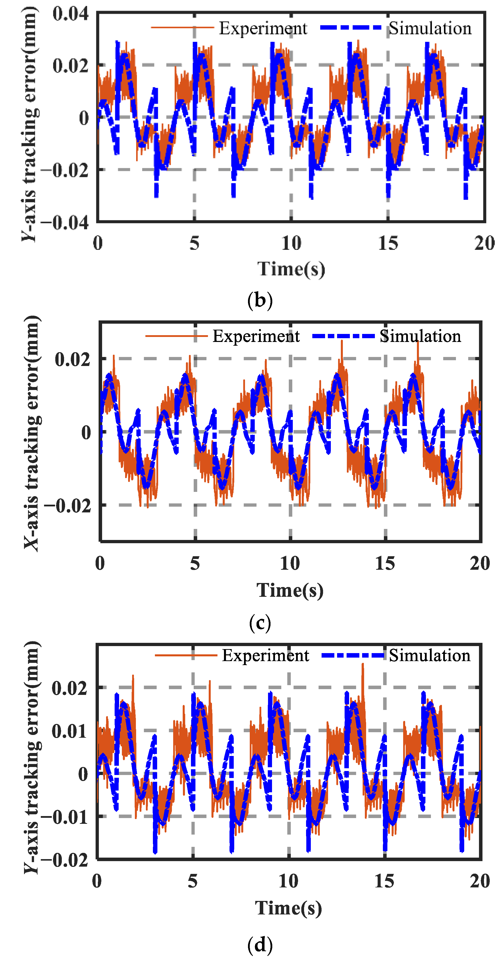
4.2. Results of the Nonlinear Dynamic Model

The sampling data are collected from the real-time running PSRM control system, consisting of the thrust force (i.e., the control action command) and the position. For each-axis model, the sampling data contain 50,000 data points; 200,000 data points are used for model identification (i.e., model training). The data used in the model training contain sufficient fluctuation information to reflect the dynamic behavior of the PSRM more comprehensively.

According to the linear expression of the PSRM, the order of the linear transfer function of the system is 2. In order to determine a suitable nonlinear module structure, different nonlinear models with different hidden layer nodes under the same linear module are identified and the corresponding results are listed in

Table 2. Comparison of the Hammerstein–Wiener model with different nonlinear modules.

Hidden Layer Nodes	Zero Order of Linear Module	Pole Order of Linear Module	RMSE
3	2	2	0.395
4	2	2	0.218
5	2	2	0.116
6	2	2	0.107
7	2	2	0.104

.

It is noted that the more complex the neural network structure is, the more infinitely it can approach the identified plant; however, it will also increase the risk of model over-fitting. By comparing the model identification results under different neural network structures in Table 2, it can be seen that when the complexity of the neural network is gradually increased, the fitting effect of the model on the training data gradually rises; when the number of hidden layer nodes of the neural network is greater than 5, the root mean square error (RMSE) decreases gradually. Considering the complexity and training effect of the model, the Hammerstein–Wiener model with five hidden layer nodes is selected as the nonlinear dynamic model for the PSRM.

With the testing data, the Hammerstein–Wiener model with five hidden layer nodes is further verified and compared with the linear dynamic model as shown in (2). The related results are listed in

Table 3. Model position error under different dynamic models.

Dynamic Model	Linear Model	Nonlinear Model	Reduction Rate (%)
${\left|e\right|}_{max}$ of X-axis (mm)	0.0500	0.0275	44.801
${\left|e\right|}_{max}$ of Y-axis (mm)	0.0691	0.0374	45.876
SMAPE of X-axis (%)	0.341	0.045	86.804
SMAPE of Y-axis (%)	1.014	0.142	85.996

. The error between the linear dynamic model output and the actual position is presented in Figure 6 and Figure 7 illustrates the error between the nonlinear dynamic model output and the actual position. According to Table 3, the X- and Y-axis maximum absolute errors between the linear dynamic model output and the actual position are 0.0500 and 0.0691 mm, respectively; the X- and Y-axis maximum absolute position errors between the nonlinear dynamic model output and the actual position are 0.0275 and 0.0374 mm, respectively, which are relatively reduced by 44.801% and 45.876%, respectively, compared to the linear dynamic model. In the linear dynamic model, the X- and Y-axis symmetrical mean absolute percentage errors (SMAPEs) are 0.341% and 1.014%, respectively. In the nonlinear dynamic model, the X- and Y-axis SMAPEs are 0.045% and 0.142%, respectively, which are relatively reduced by 86.804% and 85.996%, respectively, compared with the linear dynamic model. The developed nonlinear Hammerstein–Wiener model is demonstrated effectively and can be used as the controlled plant for the position control parameter optimization system of PSRMs.

4.3. Results of Position Control Parameter Optimization

A position control system of the PSRM is constructed based on MATLAB/Simulation, in which the model predictive control method is applied to develop the X- and Y-axis independent position controllers and the SAAPSO algorithm is used to obtain the optimal control parameters of the PSRM control system. The weight matrix Q1 and Q2 of the model predictive controller are the position control parameters to be optimized. For the SAAPSO algorithm, the population size is chosen as 25; the maximum number of iterations is set to 150; the upper and lower limits of the inertia weight changed with the similarity of particles are set to 0.9 and 0.4, respectively; the upper and lower limits of the learning factor are set to 2.5 and 1, respectively; and the temperature rise control parameter is set to 1.1.

The position control parameters obtained from the proposed method and the empirical method-based manual debugging (EMBMD) are employed in the circular and diamond trajectory tracking of the PSRM system. The X- and Y-axis position control parameters obtained by the proposed method for circular trajectory tracking are Q1 = 14.245 and Q2 = 0.024 as well as Q1 = 16.984 and Q2 = 0.020, respectively; those for diamond trajectory tracking are Q1 = 12.461 and Q2 = 0.023 as well as Q1 = 18.742 and Q2 = 0.019, respectively.

For the circular trajectory tracking, the X- and Y-axis trajectory tracking errors results using the proposed method and the EMBMD are shown in Figure 8. The related results are listed in

Table 4. Comparative results of the proposed method EMBMD and the method in [9].

Reference Trajectory	Direction	Tracking Error for EMBMD (mm)		Tracking Error for Proposed Method (mm)		Tracking Error in [9] (mm)
		${\left|e\right|}_{max}$	${\left|e\right|}_{mean}$	${\left|e\right|}_{max}$	${\left|e\right|}_{mean}$	${\left|e\right|}_{max}$	${\left|e\right|}_{mean}$
Circular trajectory	X-axis	0.0323	0.0156	0.0187	0.0083	0.0280	0.0112
	Y-axis	0.0557	0.0217	0.0248	0.0109	0.0293	0.0096
Diamond trajectory	X-axis	0.0311	0.0131	0.0249	0.0085	0.0275	0.0111
	Y-axis	0.0296	0.0115	0.0255	0.0079	0.0290	0.0092

. Figure 8a,b illustrates the corresponding X- and Y-axis tracking error results under the best position control parameters obtained by empirical-method-based manual debugging. Figure 8c,d depicts the related X- and Y-axis tracking error results under the optimal position control parameters obtained by the proposed method. The X- and Y-axis maximum absolute value position errors (denoted as |e|_max) using the EMBMD are 0.0323 and 0.0557 mm, respectively; those using the proposed method are 0.0187 and 0.0248 mm, respectively, which are reduced by 42.105% and 55.476% compared to the EMBMD, respectively. The X- and Y-axis average absolute errors (denoted as |e|_mean) using the EMBMD are 0.0156 and 0.0217 mm, respectively; those using the proposed method are 0.0083 and 0.0109 mm, respectively, which are reduced by 46.795% and 49.769% compared with the EMBMD, respectively.

For the diamond trajectory tracking, the X- and Y-axis trajectory tracking errors results, using the proposed method and the EMBMD, are shown in Figure 9. Table 4 gives the corresponding results. Figure 9a,b presents the related X- and Y-axis tracking error results under the best position control parameters obtained by EMBMD. Figure 9c,d illustrates the related X- and Y-axis tracking error results under the optimal position control parameters obtained by the proposed method. The X- and Y-axis |e|_max using the EMBMD are 0.0311 and 0.0296 mm, respectively; those using the proposed method are 0.0249 and 0.0255 mm, respectively, which are decreased by 19.935% and 16.465% compared to the EMBMD, respectively. The X- and Y-axis |e|_mean using the EMBMD are 0.0131 and 0.0115 mm, respectively, and those using the proposed method are 0.0085 and 0.0079 mm, respectively, which are decreased by 35.114% and 31.304% compared with the EMBMD, respectively.

To further verify the superiority of the proposed position control parameter optimization method, a comparison of the proposed method and the method in [9] is performed under the same trajectory tracking and the position controller with MPC. The related results are listed in Table 4. Compared with [9], the X- and Y-axis |e|_max using the proposed method in circular trajectory are reduced by 49.733% and 18.145%, respectively, and those in diamond trajectory are reduced by 10.442% and 13.725%, respectively.

4.4. Discussion

Two aspects are worth noting on the proposed nonlinear dynamic model-based position control parameter optimization method of PSRMs for practical applications, as listed below.

First, the proposed method is still valid when the time delay occurs in the considered system, which is explained as follows. The development process of the proposed method includes two steps. The first is to establish a nonlinear model and the second is to set up the control system for optimizing the control parameters. For the nonlinear modeling, the time delay may occur in the data collection process. The modeling is established based on the collected data and the collected data reflect the actual system. Therefore, the established nonlinear dynamic model, including the actual time-delay information, can represent the actual system behavior and is suitable for setting up the control system to optimize the control parameters. In addition, there is an inevitable time delay in the control system. In general, the time delay can be effectively solved using the compensation or control approaches. The control system is developed based on the compensation or control approaches to solve the time delay problem. Then, the optimization method is applied in the developed control system to obtain the optimal control parameters. The proposed method can be used as long as the control system is developed.

Second, there are two main limitations of the proposed method in practical applications (1) The proposed method belongs to the offline optimization method and thus the developed nonlinear model should be as close as possible to the actual system to accurately describe the system behavior. Moreover, the nonlinear model is built based on the collected data. As a result, there is a strict requirement for data collection. For a system with significant changing parameters or disturbances, it is necessary to cover the experimental data for almost all operating conditions as much as possible to build the nonlinear model; in addition, the nonlinear model can be built based on the experimental data collected under a specific operating condition; however, the model accuracy is relatively low for other operating conditions. (2) Constructing a control system is the prerequisite for optimizing control parameters. Therefore, the control system must be known to the user to apply the proposed method. This method cannot be applied to the unknown internal structure of control systems.

5. Conclusions

The nonlinear dynamic model-based position control parameter optimization method for PSRMs was proposed in this article. The nonlinear dynamic model of PSRMs was developed using the multi-input and multi-output Hammerstein–Wiener model structure, in which the BP neural network was applied as the nonlinear input and output modules of the model. The position control parameter optimization system of PSRMs was exploited with the developed nonlinear dynamic model. Based on the position control parameter optimization system, the SAAPSO was designed to optimize the control parameters of the position controller. The experimental results show that compared with the linear dynamic models, the X- and Y-axis maximum position errors between the nonlinear dynamic model output and the actual position are reduced by 44.801% and 45.876%, respectively, and the X- and Y-axis SMAPEs are reduced by 86.804% and 85.996%, respectively; compared to the EMBMD, the X- and Y-axis |e|_max for the proposed method under circular trajectory tracking are reduced by 42.105% and 55.476%, respectively, and those under diamond trajectory tracking are reduced by 19.935% and 16.465%, respectively; and compared with the method in [9], the X- and Y-axis |e|_max for the proposed method under circular trajectory tracking are reduced by 49.733% and 18.145%, respectively, and those under diamond trajectory tracking are reduced by 10.442% and 13.725%, respectively. The effectiveness of the proposed nonlinear dynamic model and position control parameter optimization method is verified experimentally. It is noted that the proposed method can also be applied to other types of position control motor systems to improve the control performance.

References

1. Wang, Z.; Cao, X.; Deng, Z.; Li, K. Modeling and Characteristic Investigation of Axial Reluctance Force for Bearingless Switched Reluctance Motor. IEEE Trans. Ind. Appl. 2021, 57, 5215–5226. [Google Scholar] [CrossRef]
2. Chen, N.; Cao, G.; Huang, S.; Sun, J. Sensorless Control of Planar Switched Reluctance Motors Based on Voltage Injection Combined with Core-Loss Calculation. IEEE Trans. Ind. Electron. 2020, 67, 6031–6042. [Google Scholar] [CrossRef]
3. Takayama, K.; Takasaki, Y.; Ueda, R. A new type switched reluctance motor. In Proceedings of the 1988 IEEE Industry Applications Society Annual Meeting, Pittsburgh, PA, USA, 2–7 October 1988; pp. 71–78. [Google Scholar]
4. Pan, J.; Cheung, N.; Yang, J. High-precision position control of a novel planar switched reluctance motor. IEEE Trans. Ind. Electron. 2005, 52, 1644–1652. [Google Scholar] [CrossRef]
5. Huang, S.D.; Cao, G.Z.; Peng, Y.; Wu, C.; Liang, D.; He, J. Design and analysis of a long-stroke planar switched reluctance motor for positioning applications. IEEE Access 2019, 7, 22976–22987. [Google Scholar] [CrossRef]
6. Guo, L.; Zhang, H.; Galea, M.; Li, J.; Gerada, C. Multiobjective optimization of a magnetically levitated planar motor with multilayer windings. IEEE Trans. Ind. Electron. 2016, 63, 3522–3532. [Google Scholar] [CrossRef]
7. Ou, T.; Hu, C.; Zhu, Y.; Zhang, M.; Zhu, L. Intelligent feedforward compensation motion control of maglev planar motor with precise reference modification prediction. IEEE Trans. Ind. Electron. 2020, 68, 7768–7777. [Google Scholar] [CrossRef]
8. Huang, S.; Chen, L.; Cao, G.; Wu, C.; Xu, J.; He, Z. Predictive position control of planar motors using trajectory gradient soft constraint with attenuation coefficients in the weighting matrix. IEEE Trans. Ind. Electron. 2021, 68, 821–837. [Google Scholar] [CrossRef]
9. Huang, S.; Cao, G.; Xu, J.; Cui, Y.; Wu, C.; He, J. Predictive position control of long-stroke planar motors for high-precision positioning applications. IEEE Trans. Ind. Electron. 2021, 68, 796–811. [Google Scholar] [CrossRef]
10. San-Miguel, A.; Alenyà, G.; Puig, V. Automated Off-Line Generation of Stable Variable Impedance Controllers According to Performance Specifications. IEEE Robot. Autom. Lett. 2022, 7, 5874–5881. [Google Scholar] [CrossRef]
11. Xu, W.; Ismail, M.M.; Liu, Y.; Islam, M.R. Parameter Optimization of Adaptive Flux-Weakening Strategy for Permanent-Magnet Synchronous Motor Drives Based on Particle Swarm Algorithm. IEEE Trans. Power Electron. 2019, 34, 12128–12140. [Google Scholar] [CrossRef]
12. Liu, X.; Zhang, H.; Zhu, P. Identification of nonlinear state-space time-delay system. Assem. Autom. 2020, 40, 22–30. [Google Scholar] [CrossRef]
13. Vujicic, V.; Vukosavic, S.N. A simple nonlinear model of the switched reluctance motor. IEEE Trans. Energy Convers. 2000, 15, 395–400. [Google Scholar] [CrossRef] [PubMed]
14. Huang, S.; Hu, Z.; Cao, G. Input-Constrained-Nonlinear-Dynamic-Model-Based Predictive Position Control of Planar Motors. IEEE Trans. Ind. Electron. 2021, 68, 7294–7308. [Google Scholar] [CrossRef]
15. Sjöberg, J.; Zhang, Q.; Ljung, L. Nonlinear black-box modeling in system identification: A unified overview. Automatica 1995, 31, 1691–1724. [Google Scholar] [CrossRef]
16. Andonovski, G.; Lughofer, E.; Škrjanc, I. Evolving Fuzzy Model Identification of Nonlinear Wiener-Hammerstein Processes. IEEE Access 2021, 9, 158470–158480. [Google Scholar] [CrossRef]
17. Dong, J. Robust Data-Driven Iterative Learning Control for Linear-Time-Invariant and Hammerstein–Wiener Systems. IEEE Trans. Cybern. 2023, 53, 1144–1157. [Google Scholar] [CrossRef] [PubMed]
18. Kayedpour, N.; Samani, A.E.; Kooning, J.D.; Vandevelde, L.; Crevecoeur, G. Model Predictive Control with a Cascaded Hammerstein Neural Network of a Wind Turbine Providing Frequency Containment Reserve. IEEE Trans. Energy Convers. 2022, 37, 198–209. [Google Scholar] [CrossRef]
19. Zambrano, J.; Sanchis, J.; Herrero, J.M.; Martínez, M. A Unified Approach for the Identification of Wiener, Hammerstein, and Wiener–Hammerstein Models by Using WH-EA and Multistep Signals. Complexity 2020, 2020, 7132349. [Google Scholar] [CrossRef]
20. Zong, T.; Li, J.; Lu, G. Auxiliary model-based multi-innovation PSO identification for Wiener–Hammerstein systems with scarce measurements. Eng. Appl. Artif. Intell. 2021, 106, 104470. [Google Scholar] [CrossRef]
21. Khalifa, T.R.; El-Nagar, A.M.; El-Brawany, M.A.; El-Araby, E.A.; El-Bardini, M. A Novel Hammerstein Model for Nonlinear Networked Systems Based on an Interval Type-2 Fuzzy Takagi–Sugeno–Kang System. IEEE Trans. Fuzzy Syst. 2021, 29, 275–285. [Google Scholar] [CrossRef]
22. Kothari, K.; Mehta, U.; Prasad, V.; Vanualailai, J. Identification scheme for fractional Hammerstein models with the delayed Haar wavelet. IEEE/CAA J. Autom. Sin. 2020, 7, 882–891. [Google Scholar] [CrossRef]
23. Zhang, J. Disturbance-Encoding-Based Neural Hammerstein–Wiener Model for Industrial Process Predictive Control. IEEE Trans. Syst. Man Cybern. 2022, 52, 606–617. [Google Scholar] [CrossRef]
24. Han, R.; Wang, R.; Zeng, G. Identification of dynamical systems using a broad neural network and particle swarm optimization. IEEE Access 2020, 8, 132592–132602. [Google Scholar] [CrossRef]
25. Son, S.; Lee, H.; Jeong, D.; Oh, K.; Sun, K. A novel physics-informed neural network for modeling electromagnetism of a permanent magnet synchronous motor. Adv. Eng. Inform. 2023, 57, 102035. [Google Scholar] [CrossRef]
26. Pham, T.D.; Lee, Y.W.; Park, C.; Park, K.R. Deep Learning-Based Detection of Fake Multinational Banknotes in a Cross-Dataset Environment Utilizing Smartphone Cameras for Assisting Visually Impaired Individuals. Mathematics 2022, 10, 1616. [Google Scholar] [CrossRef]
27. Zheng, Y.; Huang, Z.; Tao, J.; Sun, H.; Sun, Q.; Sun, M.; Dehmer, M.; Chen, Z. A Novel Chaotic Fractional-Order Beetle Swarm Optimization Algorithm and Its Application for Load-Frequency Active Disturbance Rejection Control. IEEE Trans. Circuits Syst. II-Express Briefs. 2022, 69, 1267–1271. [Google Scholar] [CrossRef]
28. Feng, L.; Sun, X.; Tian, X.; Diao, K. Direct Torque Control with Variable Flux for an SRM Based on Hybrid Optimization Algorithm. IEEE Trans. Power Electron. 2022, 37, 6688–6697. [Google Scholar] [CrossRef]
29. Tian, M.; Gao, Y.; He, X.; Zhang, Q.; Meng, Y. Differential Evolution with Group-Based Competitive Control Parameter Setting for Numerical Optimization. Mathematics 2023, 11, 3355. [Google Scholar] [CrossRef]
30. Jin, Z.; Sun, X.; Lei, G.; Guo, Y.; Zhu, J. Sliding Mode Direct Torque Control of SPMSMs Based on a Hybrid Wolf Optimization Algorithm. IEEE Trans. Ind. Electron. 2022, 69, 4534–4544. [Google Scholar] [CrossRef]
31. Qiang, Z.; Li, C. Two-stage multi-swarm particle swarm optimizer for unconstrained and constrained global optimization. IEEE Access 2020, 8, 124905–124927. [Google Scholar]
32. Zhang, W.; Ma, J.; Wang, L.; Jiang, F. Particle-Swarm-Optimization-Based 2D Output Feedback Robust Constraint Model Predictive Control for Batch Processes. IEEE Access 2022, 10, 8409–8423. [Google Scholar] [CrossRef]
33. Xia, X.; Song, H.; Zhang, Y.; Gui, L.; Xu, X.; Li, K.; Li, Y. A Particle Swarm Optimization with Adaptive Learning Weights Tuned by a Multiple-Input Multiple-Output Fuzzy Logic Controller. IEEE Trans. Fuzzy Syst. 2023, 31, 2464–2478. [Google Scholar] [CrossRef]
34. Yang, X.; Li, H. An adaptive dynamic multi-swarm particle swarm optimization with stagnation detection and spatial exclusion for solving continuous optimization problems. Swarm Intell. 2023, 1, 33–57. [Google Scholar] [CrossRef]
35. Bonyadi, M.R. A Theoretical Guideline for Designing an Effective Adaptive Particle Swarm. IEEE Trans. Evol. Comput. 2020, 24, 57–68. [Google Scholar] [CrossRef]
36. Pozna, C.; Precup, R.E.; Horváth, E.; Petriu, E.M. Hybrid Particle Filter–Particle Swarm Optimization Algorithm and Application to Fuzzy Controlled Servo Systems. IEEE Trans. Fuzzy Syst. 2022, 30, 4286–4297. [Google Scholar] [CrossRef]
37. Li, J.; Guo, L.; Zuo, Y.; Liu, W. A Design Method for Wideband Chaff Element Using Simulated Annealing Algorithm. IEEE Antennas Wirel. Propag. Lett. 2022, 21, 1208–1212. [Google Scholar] [CrossRef]
38. Zhang, P.; Song, S.; Niu, S.; Zhang, R. A Hybrid Artificial Immune-Simulated Annealing Algorithm for Multiroute Job Shop Scheduling Problem with Continuous Limited Output Buffers. IEEE Trans. Cybern. 2022, 52, 12112–12125. [Google Scholar] [CrossRef]
39. Lee, S.; Kim, S.B. Parallel Simulated Annealing with a Greedy Algorithm for Bayesian Network Structure Learning. IEEE Trans. Knowl. Data Eng. 2020, 32, 1157–1166. [Google Scholar] [CrossRef]
Disclaimer/Publisher’s Note: The statements, opinions and data contained in all publications are solely those of the individual author(s) and contributor(s) and not of MDPI and/or the editor(s). MDPI and/or the editor(s) disclaim responsibility for any injury to people or property resulting from any ideas, methods, instructions or products referred to in the content.