Design and Optimization of a Spherical Magnetorheological Actuator

Abstract

Recently, an increasing number of electromagnetic devices have been using smart fluids. These include ferrofluids, electrorheological fluids, and magnetorheological (MR) fluids. In the paper, magnetorheological fluids are considered for use in a spherical actuator for haptic applications. An approach is presented to the design and optimization of such a device, using finite element method modelling linked with differential evolution (DE). Much consideration was given to the construction of the objective function to be minimized. A novel approach to objective function assembly was used, using reference values based on the model design and created with parameters set to the midpoint values of the selected range. It was found to be a useful strategy when the reference values are unknown. There were four parameters to be optimized. Three of them gravitated towards the boundary value, and the fourth (actuator radius) was somewhere in between. The value of the objective function reached a minimum in the range of actuator radius between 42.9880 mm and 45.0831 mm, which is about a 5% difference in regard to the actuator radius. Three passes of optimization were performed with similar results, proving the robustness of the algorithm.

1. Introduction

Nowadays, more and more electromagnetic devices use materials known as smart materials. These include so-called smart fluids, whose properties change in the presence of electric or magnetic fields. Smart fluids include ferrofluids [1], electrorheological fluids [2], and magnetorheological (MR) fluids [3]. In this paper, MR fluid was considered for use in a spherical MR actuator for haptic applications. In the development process, the actuator’s geometry was optimized using the differential evolution (DE) algorithm and finite element method (FEM) modelling to increase the actuator’s efficiency.

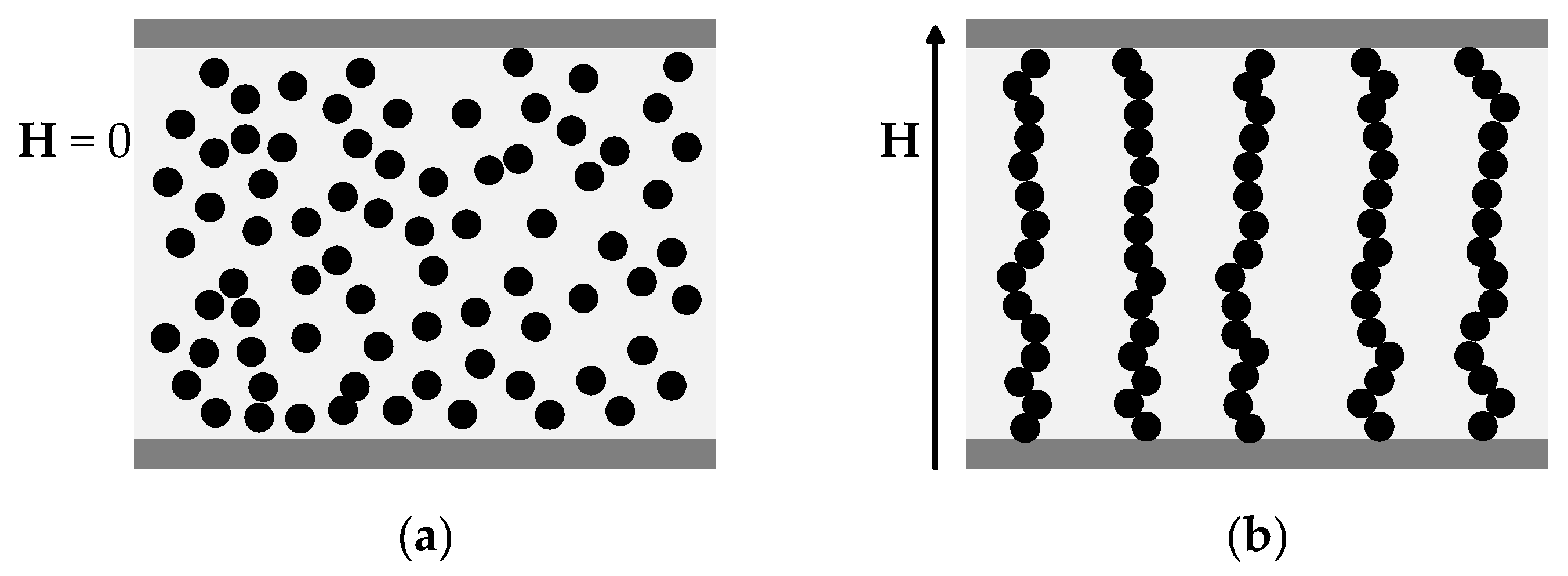
The beginning of MR fluids dates back to 1948 when they were discovered by Jacob Rabinow at the US National Bureau of Standards [4,5]. An MR fluid is a type of smart fluid whose rheological properties change in the presence of an external magnetic field. Specifically, it manifests as an increase in its viscosity. The change can be so significant that it behaves like a viscoelastic solid. MR fluid is a mixture of carrier fluid and micrometer-sized magnetic particles. The change in viscosity is attributed to the formation of chains of particles, which hinder the free flow of the surrounding fluid (Figure 1) [4].

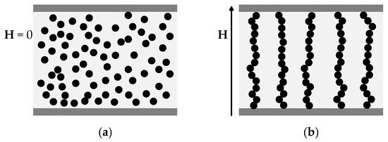
Figure 1. Schematic representation of chain formation in magnetorheological (MR) fluid. Case (a) shows the random distribution of particles in the fluid at field $\mathrm{H}=$ 0, and case (b) shows the chain formation at field $\mathrm{H}>$ 0.

A spherical MR actuator was designed and optimized in this article. The final intended use of the actuator is in haptic applications as a joystick. The user then operates the joystick and receives feedback of the braking force through it provided by the rheological changes that appear in the MR fluid due to the magnetic field provided by the excitation coil. The joystick may be used in different applications, such as video games, simulations, or robotic applications. The goal is that the generated braking force is as close to reality as possible.

For the design optimization, publications were searched with a similar design of spherical magnetorheological actuator. The resulting publications were [6,7,8,9]. In publication [6], optimization is described as a finite element analysis (FEA) to optimize the structure. Their optimization aimed to saturate the magnetic flux density acting on the MR fluid and the yoke structure. No specific design optimization is described in [7,8,9]. Due to lacking a design optimization process description, the search parameters for publications were extended to MR actuators operating in shear mode, such as rotary brakes and clutches. Different approaches to design optimization have been used regarding optimization goals and algorithms. Popular optimization goals for MR actuators are the maximization of torque and minimization of mass, as in [10], where the authors used simulated annealing with sequential quadratic programming, and in [11], using only simulated annealing. With the same goals, the authors in [12,13] used the genetic algorithm. In addition to torque and mass, in [14], the authors optimized a magnetic circle using the particle swarm algorithm. In [15], the genetic algorithm with sequential quadratic programming was used to optimize the torque, response time, and mass of an MR brake. In [16], they optimized a serpentine flux brake for the highest magnetic flux density, making incremental changes in the design parameters. In [17], they used the multi-objective genetic algorithm (MOGA) for off-state torque minimization and braking torque maximization of an MR disc brake. Other optimization approaches use the Nealder–Mead algorithm for new parameter generation, as in [18]; the Taguchi method combined with FEM [19]; and built-in optimization tools in FEM software. For instance, ANSYS was used in [20]. In constructing the objective function for the optimization process, the authors in [10,11,12,13,15] used reference values of certain quantities for normalization. In [11,12,15], the reference values were chosen as a specific value; in [13], the reference values were calculated based on a random design within the constraints; and in [10], the reference value for torque was selected based on several random models, and the reference value for weight was obtained considering the overall system weight of a similar conventional (non-MR) device. In this paper, the reference values were calculated based on a design with parameters set on the midpoint between the lower and upper boundary values. Such a strategy was not used in other publications. It is a useful strategy when the reference values are not known.

The DE algorithm was selected for the optimization of the spherical MR actuator in this study. DE is an evolutionary optimization algorithm. It is an iterative process that searches for an optimal solution to a problem based on imitation of natural evolutionary processes. In each iteration (called generation), there are $NP$ population members. The working principle of DE is as follows [21]. First, the lower and upper bounds are specified for the parameters. These define the domain from which the population members can be taken. Then, the population is initialized so that the parameters of each population member are selected randomly from the domain. After initialization, the DE mutates and recombines the population to produce a population of $NP$ mutant vectors. For example, the creation of a mutant vector ${\mathrm{v}}_{i,g}$ ($i$ is the index denoting a member within a population, and $g$ is the index denoting the generation) from three randomly chosen population members (${\mathrm{x}}_{r0,g}$, ${\mathrm{x}}_{r1,g}$, and ${\mathrm{x}}_{r2,g}$; $r$ specifies that the vector is chosen randomly) is shown with Equation (1):

$${\mathrm{v}}_{i,g}={\mathrm{x}}_{r0,g}+F\left({\mathrm{x}}_{r1,g}-{\mathrm{x}}_{r2,g}\right).$$

(1)

Factor $F$ is the scale factor and is a positive real number, usually lower than 1. The mutation is complemented with crossover. Crossover builds a trial vector from the parameters of two vectors; specifically, it crosses each population member with the corresponding mutant vector. The probability of crossover is defined with the parameter $CR$. It has a value between 0 and 1. To select which parameters come from which vector, $CR$ is compared to the output of a random number generator. If the random value is lower or equal to $CR$, the trial function inherits the component value from the mutant vector; otherwise, it inherits it from the population member. In addition, a randomly chosen component from the mutant vector is chosen for the trial vector so that the trial vector is not the same as the population member. For the selection of the next generation population members, the value of the objective function of the trial vector is compared to the value of the objective function of the corresponding population member. If the value of the former is lower or equal to the latter’s, the trial vector replaces the population member in the next generation; otherwise, the population member stays the same. The process repeats itself until the optimal solution is found or a termination criterion is satisfied (e.g., the maximum number of iterations).

There are different possible strategies for DE. They differ in the way they calculate the trial vector. The strategies are notated as DE/p1/p2/p3. DE stands for differential evolution. String p1 defines how the vector to be perturbed is selected. Typically, rand or best is selected (rand—random vector, best—best vector). Number p2 defines the number of difference vectors used for perturbation. String p3 defines the type of crossover (e.g., exp for exponential or bin for binomial). For example, the notation for the strategy used in this publication is DE/rand/1/exp. The selection of this strategy was made based on experience. In [22], three strategies (DE/rand/1exp, DE/rand/2/exp and DE/best/1/bin) were compared, and in [23], two strategies were compared (DE/rand/1/exp and DE/rand/2/exp). In both, DE/rand/1/exp proved to be the best choice.

The main contributions of this work are:

• Design of a spherical MR actuator within given geometric and magnetic constraints;
• Development of a parametric FEM model which offers the possibility of coupling between the optimization method and the FEM model;
• Suitable combination of the analytical torque equations with the values resulting from the FEM analysis of the model for torque calculations;
• Approach to the optimization of the geometry of a spherical MR actuator;
• Construction of the objective function in the context of a spherical MR actuator optimization, which provides as big as possible a torque, as small as possible dimensions, and the required magnetic flux density in the actuator;
• A novel approach to objective function assembly, with the use of reference values based on the model design created with the midpoint parameter values.

The paper continues with Section 2 (Materials and Methods), describing the designing and optimization processes in Section 2.1 and Section 2.2, respectively. In Section 2.3, a verification of the FEM model is presented. The results achieved with these processes are presented in Section 3. The conclusions are presented in Section 4.

2. Materials and Methods

2.1. Design and Parametrization

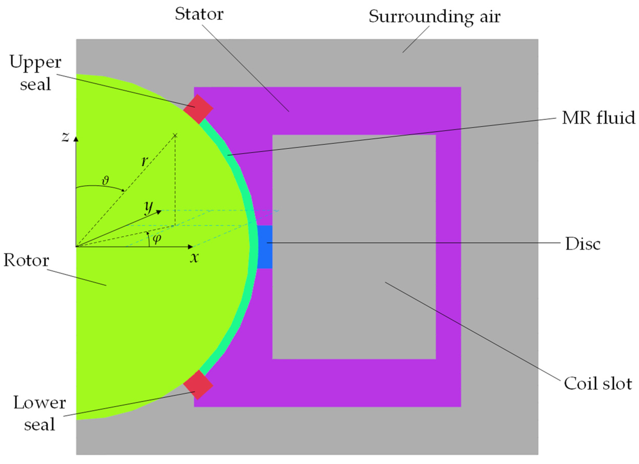
The goal was to design a small spherical MR actuator intended for use in haptic interfaces as a joystick. A spherical coordinate system was used for the design and analysis of the results (Figure 2).

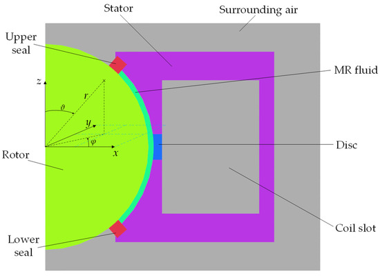
Figure 2. Cross-section of half of the actuator model and the coordinate system used in the analysis.

The basic design consisted of a spherical rotor, a stator, an aluminum disc, a coil, MR fluid, and upper and lower seals. The layout is presented in Figure 2. The materials defined for the individual components are presented in Table 1.

Table 1. Actuator components and their materials.

Component	Material
Rotor and stator	AISI 1018 low carbon steel
MR fluid	Magnaflo+ MR fluid from Arus MR Tech
Seal	Polytetrafluoroethylene (PTFE)
Disc	Aluminum

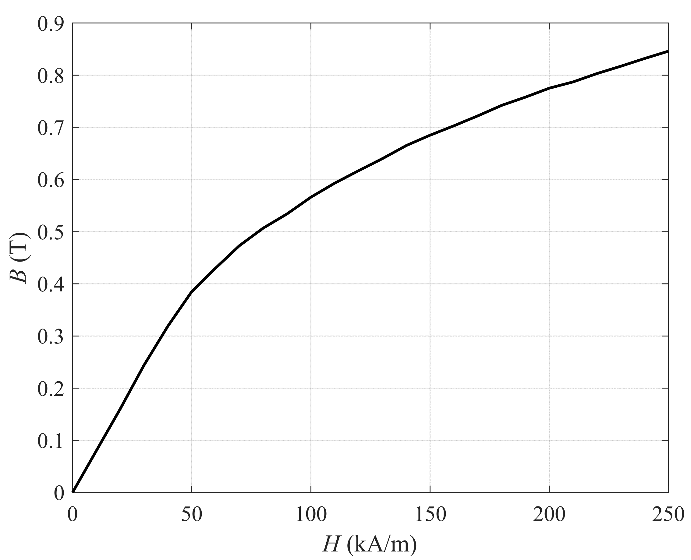
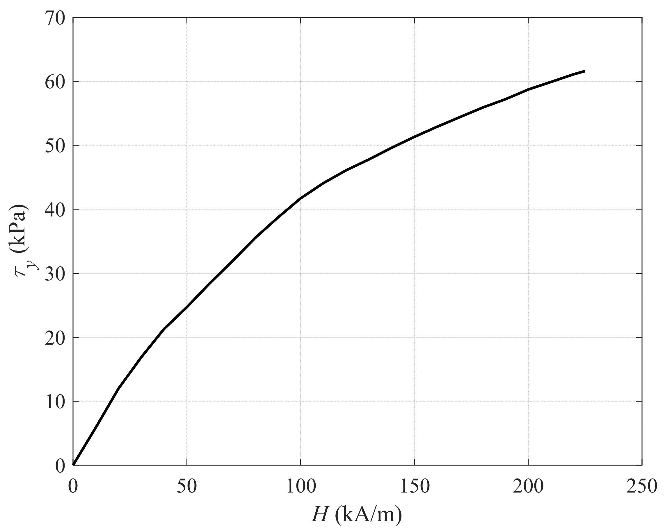
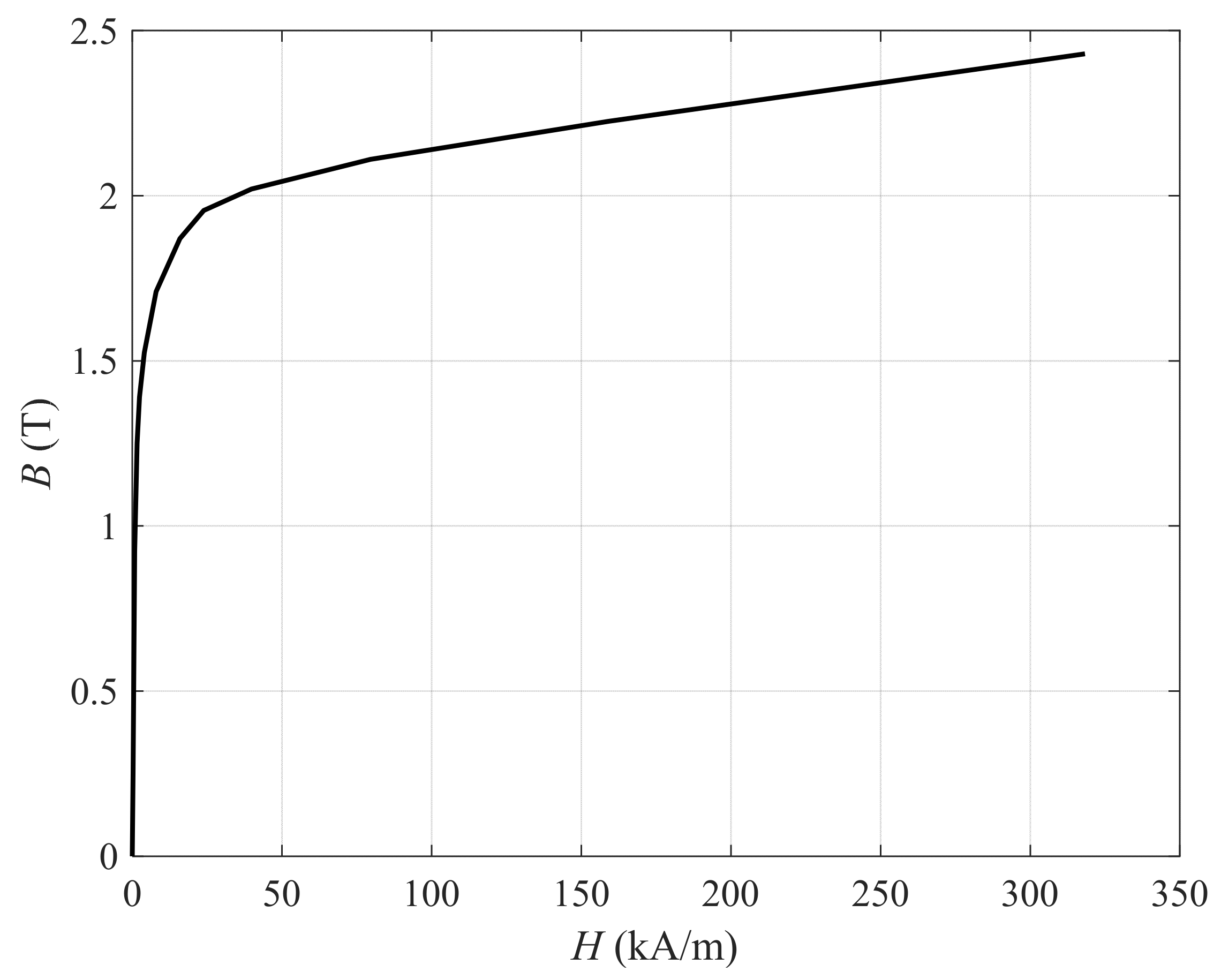
The MR fluid used was the commercially available MR fluid AMT—Magnaflo⁺ from Arus MR Tech. Figure 3 presents the magnetization curve of the MR fluid, and Figure 4 presents its yield stress curve.

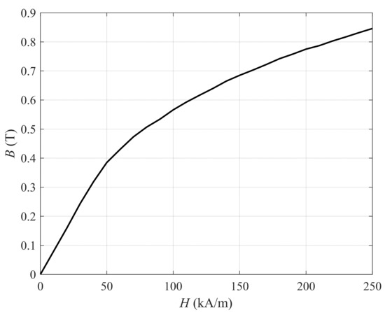
Figure 3. Magnetization curve of Magnaflo⁺ MR fluid, obtained from its datasheet [24].

Figure 4. Yield stress dependence on magnetic field strength for Magnaflo⁺ MR fluid, obtained from its datasheet [24].

Figure 5 presents the magnetization curve of AISI 1018 steel used for the stator and rotor.

Figure 5. Magnetization curve of AISI 1018 steel, obtained from [10].

Some of the parameters were defined as constants based on the desired dimensions or constraints. These are presented in Table 2.

Table 2. Parameters that are defined as constants.

Parameter	Value
Rotor radius—$r_r$	20 mm
MR fluid thickness—$d_{MR}$	1 mm
Maximum offset of the joystick (at joystick thickness of 5 mm)—${\vartheta }_{os}$	30°
Position of the aluminum disc—${\vartheta }_d$	90°
Seal thickness—$d_s$	2.5 mm
Desired magnetic flux density in the MR fluid—$B_{MR}$	0.8 T
Desired magnetic flux density in the stator—$B_S$	1.8 T

The radius of the rotor was selected to be constant at 20 mm, and the thickness of the MR fluid was set to 1 mm to ensure a sufficiently small gap between the stator and rotor and to allow for manufacturing variances. The maximum offset of the joystick was such that it allowed for an adequate range of motion when in use. The aluminum disc position was set to 90° to the vertical axis. The upper and lower seals were positioned symmetrically over the horizontal plane that divides the rotor in half. The thickness of the seal was set to 2.5 mm as a working dimension and could be subject to change in later iterations of the actuator. Four parameters were subject to optimization. These were the upper dimension (the distance from the rotor’s center to the stator’s top), the lower dimension (the distance from the rotor’s center to the stator’s bottom), the radius of the actuator, and the thickness of the aluminum disc. The dimensional bounds of these parameters are presented in Table 3.

Table 3. Parameters subject to optimization.

Parameter	Lower Bound (mm)	Upper Bound (mm)
Upper dimension—$h_u$	18.5	30
Lower dimension—$h_l$	18.5	30
Actuator radius—$r_a$	35	50
Disc thickness—$d_d$	0.5	5

The dimensions of the elements are shown in Figure 6.

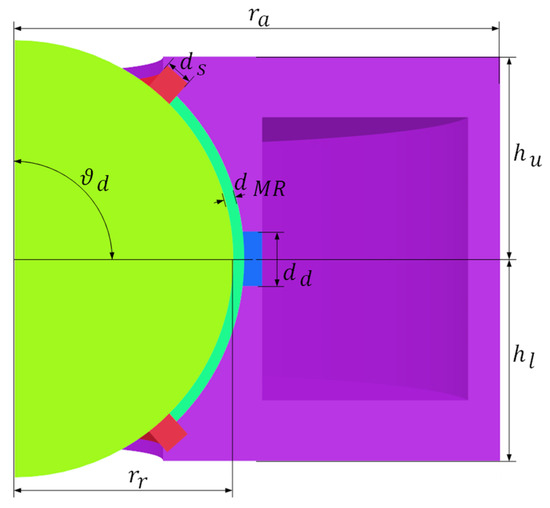
Figure 6. Representation of the parameters’ dimensions.

Every other structural parameter was calculated using previously defined parameters. These structural parameters are shown in Figure 7.

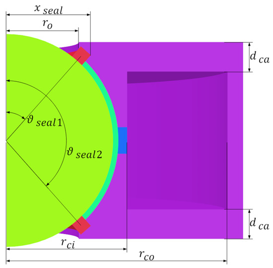
Figure 7. Structural parameters used for model building.

There is a cutout in the stator above and below the rotor (symmetrical). The radius of the cutout ($r_o$) was defined with the maximum offset of the joystick as follows:

$$r_o=h_u\tan \left({\vartheta }_{os}\right)+\frac{r_{js}}{\cos \left({\vartheta }_{os}\right)}.$$

(2)

Parameter $r_{js}$ is the cross-section radius of the joystick. It was defined with a value of 2.5 mm.

The seal position was defined as an angle of the center line of the seal. It was defined so that the center line of the seal and the vertical line at $r_o$ intersect at half the thickness of the MR fluid. It was calculated using the cutout radius and rotor radius with half of the thickness of the MR fluid added:

$${\vartheta }_{seal1}=\mathrm{asin}\left(\frac{r_o}{r_r+d_{MR}/2}\right).$$

(3)

The resulting angle ${\vartheta }_{seal1}$ is the angle of the upper seal position. Since the lower seal position is symmetric, the lower seal position, in degrees, was calculated as:

$${\vartheta }_{seal2}=180°-{\vartheta }_{seal1}.$$

(4)

The dimensions of the coil were calculated with the following method. The magnetic flux through the magnetic path shown in Figure 8 must be constant, meaning that the product $BA$, where $B$ is magnetic flux density and $A$ is the area, must be constant.

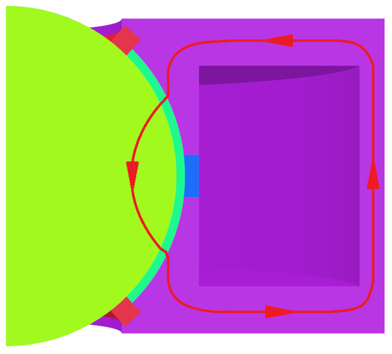
Figure 8. Schematic representation of the magnetic flux path.

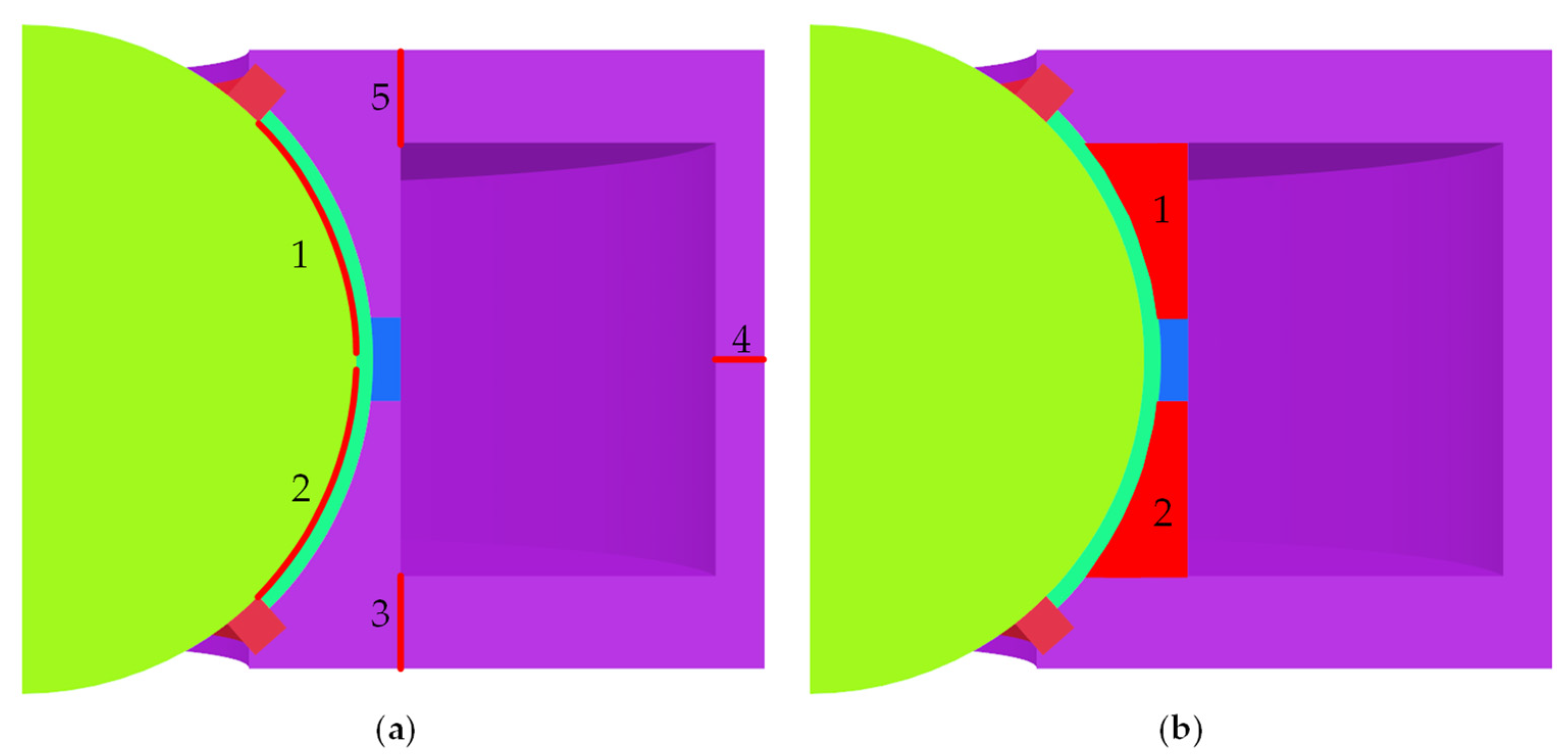
Based on that, critical sectors of the actuator were selected (Figure 9a), where it was assumed that:

$$B_i{A}_i=B_j{A}_j.$$

(5)

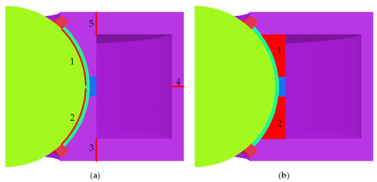
Figure 9. (a) Selected critical sectors of the actuator and numbered from 1–5, (b) Selected critical regions of the actuator and numbered from 1–2.

Indices $i$ and $j$ denote individual sectors from Figure 9a.

Magnetic flux $\varphi$ through sector 1 (the result is the same for sector 2) was defined as:

$${\varphi }_1=A_1{B}_1,$$

(6)

where, for $B_1$, the desired magnetic flux density in MR fluid $B_{MR}$ was used. $A_1$ is the surface area of sector 1. It was calculated as follows:

$$A_1={{\displaystyle \int }}_{{\vartheta }_1}^{{\vartheta }_2}2\pi r_r^2\sin \left(\vartheta \right)\mathrm{d}\vartheta .$$

(7)

Angle ${\vartheta }_2={\vartheta }_d$, and angle ${\vartheta }_1$ is the angle at which the MR fluid starts (the angle where the rotor, MR fluid, and upper seal meet). For the lower part of the rotor, $A_2=A_1$.

Since $\varphi$ is the same through all of the sectors, area $A_i$ (for $i=$ 3, 4, 5) was calculated as:

$$A_i=\frac{{\varphi }_1}{B_i},$$

(8)

where $B_i=B_S$. Using this, the distance from the actuator’s edge to the edge of the coil, $d_{ca}$, was evaluated for the upper and lower parts of the actuator. Distance $d_{ca}$ was calculated using area $A_3$ (or $A_5$) and the inner radius of the coil $r_{ci}$ (Equations (13)–(15)). Areas $A_3$ and $A_5$, expressed with $r_{ci}$ and $d_{ca}$, are:

$$A_3=A_5=2\pi r_{ci}{d}_{ca}.$$

(9)

Using Equations (6)–(9), $d_{ca}$ was expressed as:

$$d_{ca}=\frac{B_{MR}{r}_r^2\left(\cos \left({\vartheta }_1\right)-\cos \left({\vartheta }_d\right)\right)}{B_S{r}_{ci}}.$$

(10)

Area $A_4$, expressed with coil and actuator dimensions, is:

$$A_4=\pi \left(r_a^2-r_{co}^2\right),$$

(11)

where $r_{co}$ is the outer radius of the coil. Considering Equations (6)–(8) and (11), $r_{co}$ was calculated as:

$$r_{co}=\sqrt{r_a^2-\frac{B_{MR}}{B_S}2r_r^2\left(\cos \left({\vartheta }_1\right)-\cos \left({\vartheta }_d\right)\right)}.$$

(12)

Radius $r_{ci}$ was calculated in so that the magnetic flux density in regions 1 and 2 (Figure 9b) did not exceed the desired magnetic flux density of the stator. It was calculated as follows:

$$r_{ci}=\sqrt{2\frac{B_{MR}}{B_S}{r}_r^2\left(\cos \left({\vartheta }_d\right)+\frac{B_{MR}}{B_S}\frac{r_r^2}{{\left(r_r+d_{MR}\right)}^2}\right)+{\left(r_r+d_{MR}\right)}^2{\sin }^2\left(\mathrm{acos}\left(-\frac{B_{MR}}{B_S}\frac{r_r^2}{{\left(r_r+d_{MR}\right)}^2}\right)\right)}.$$

(13)

If the magnetic flux density between the outermost point of the seal and the coil, $B_{s-c}$ (Equation (14) ((Equation (14) is valid if the height of the outermost part of the seal is the same or lower than the upper edge of the coil. Otherwise, $r_{ci}$ is calculated with Equation (13) and calculating $B_{s-c}$ is unnecessary), exceeded $B_S$, $r_{ci}$ was calculated with Equation (15).

$$B_{s-c}=\frac{{\varphi }_1}{\pi \left(r_{ci}^2-x_{seal}^2\right)},$$

(14)

where $x_{seal}$ is the outermost point of the seal.

$$r_{ci}=\sqrt{\frac{{\varphi }_1}{\pi B_S}+x_{seal}^2}.$$

(15)

The aluminum disc had a center aligned with the rotor center. A spherical shape of radius $r_r+d_{MR}$ was used to cut out the inner part of the disc while the outer radius of the disc coincided with the inner radius of the coil.

2.2. Model Optimization

For optimization, the DE was used to find the minimum of an objective function with multiple objectives. The DE/rand/1/exp strategy was deployed for the search for a candidate solution. Factors $F$ and $CR$ were chosen as: $F$ = 0.6 and $CR$ = 0.8. The strategy and the values of the factors were chosen based on experience [22,23]. The number of population members was set to $NP$ = 20. The parameters subject to optimization were: upper dimension of the stator—$h_u$, lower dimension of the stator—$h_l$, actuator radius—$r_a$, and aluminum disc thickness—$d_d$.

The optimization algorithm was used in conjunction with FEM analysis. Matlab was used with Simulia Opera to build a 3D model and solve a magnetostatic problem using FEM analysis.

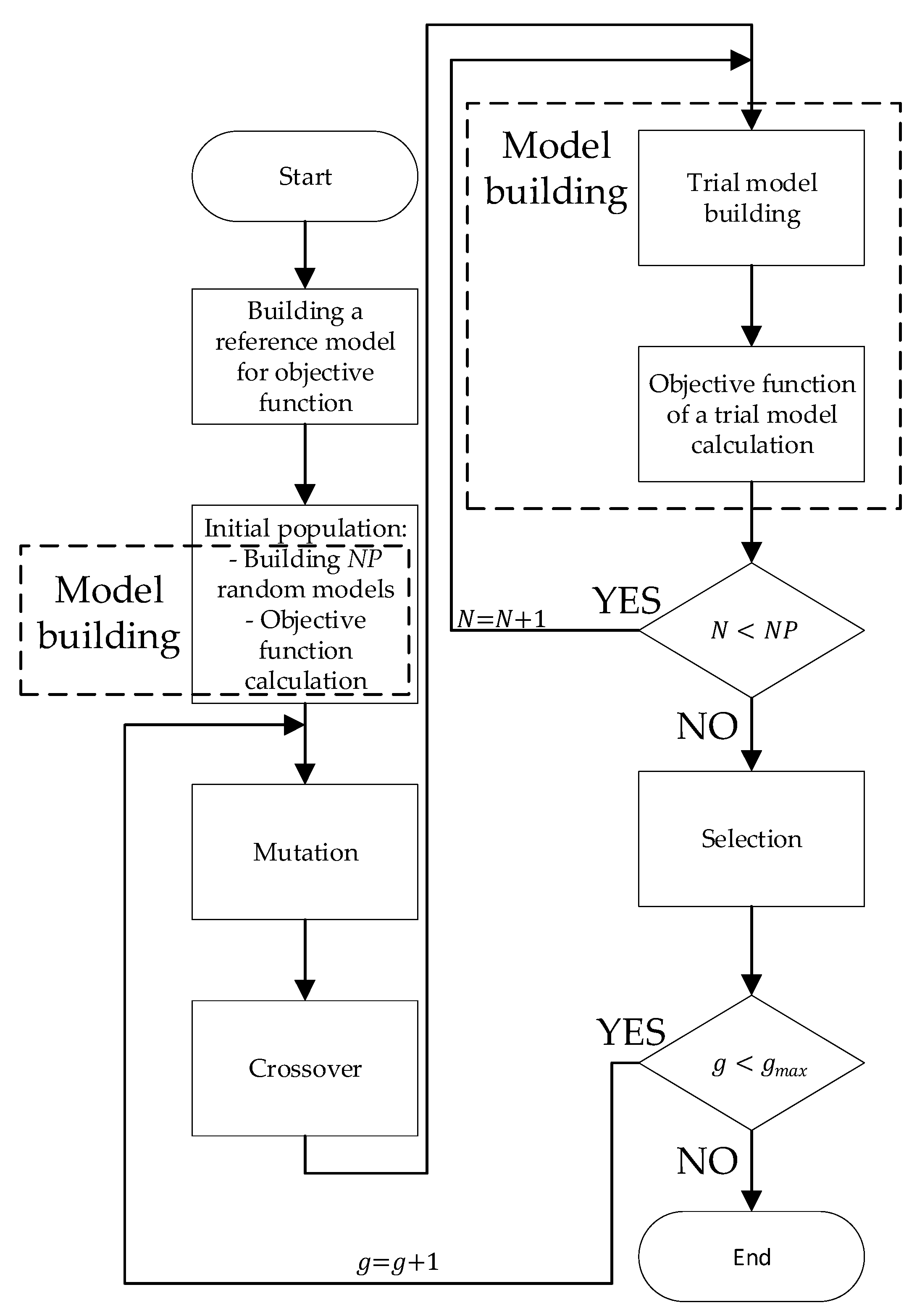
First, the reference model was created (used for objective function determination) and analyzed to initialize the optimization process, after which the initial population was made using random values between the boundary values of the four parameters. For each new population, 20 more models had to be created, analyzed, and compared to the previous population. The optimization process was finished if the best candidate stayed the same in 20 consecutive iterations or the number of iterations reached the maximum allowed iterations, defined as 100. Figure 10 shows the flowchart of the optimization process.

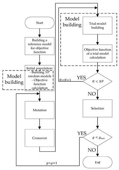
Figure 10. Flowchart of the differential evolution (DE) for spherical MR actuator design. Number $g$ is the current generation index, and $g_{max}$ is the maximum iteration number.

2.2.1. Objective Function

For objective function calculation of individual models, the reference model was first built from the midpoint values of parameters $h_u$, $h_l$, $r_a$, and $d_d$ (Table 4). The reason was to get reference values of certain results used in the objective function to make the objective function dimensionless and ensure a suitable weighting of the quantities with different units and sizes.

Table 4. Midpoint values of the parameters subject to optimization, based on which the reference model was built.

Parameter	Midpoint Value (mm)
$h_u$	24.25
$h_l$	24.25
$r_a$	42.5
$d_d$	2.75

The objective function was constructed with multiple objectives in mind. Several optimization objectives were chosen:

• Maximization of torque,
• Minimization of the size,
• Getting the desired magnetic flux density at critical areas.

The resulting function consisted of three main parts; each weighed differently based on the assigned importance of the individual part. The general form of the objective function was:

$$f=w_1{P}_1+w_2{P}_2+w_3{P}_3,$$

(16)

where $P_1$, $P_2$, and $P_3$ are the sub-objective functions, and $w_1$, $w_2$, and $w_3$ are the weights. The sub-objective functions were defined individually as follows. $P_1$ aimed to maximize the torque and minimize the magnetic flux density in the aluminum ring:

$$P_1=\frac{1}{3}\left(\frac{B_d-B_{dr}}{B_{dr}}+\frac{T_{zr}-T_z}{T_{zr}}+\frac{T_{xyr}-T_{xy}}{T_{xyr}}\right).$$

(17)

$B_d$ is the magnetic flux density in the aluminum disc, $T_z$ is the torque for rotation around the vertical axis, and $T_{xy}$ is the torque for movement in the $xy$ plane. $B_{dr}$, $T_{zr}$, and $T_{xyr}$ are their respective reference values. The value 1/3 represents the weight of the individual part of the function $P_1$. $P_2$ was the function representing the size of the actuator:

$$P_2=w_{21}\frac{r_a-r_{ar}}{r_{ar}}+w_{22}\frac{h_s-h_{sr}}{h_{sr}},$$

(18)

where $h_s=h_u+h_l$ is the stator height, $h_{sr}$ is its reference value, and $r_{ar}$ is the reference value of the actuator radius. Values $w_{21}$ and $w_{22}$ are the weights for the function. $P_3$ consisted of the desired magnetic flux densities at five critical regions:

$$P_3=\frac{1}{5}\left(\frac{\left|B_1-B_{MR}\right|}{B_{MR}}+\frac{\left|B_2-B_{MR}\right|}{B_{MR}}+\frac{\left|B_3-B_S\right|}{B_S}+\frac{\left|B_4-B_S\right|}{B_S}+\frac{\left|B_5-B_S\right|}{B_S}\right).$$

(19)

$B_i$, for $i=$ 1, 2, 3, 4, 5, is the magnetic flux density at the critical sectors (Figure 9a). The value 1/5 is the weight of each part of the function $P_3$. Table 5 shows the values for the weights $w_1$, $w_2$, $w_3$, $w_{21}$, and $w_{22}$. All the values of the weights were selected so that the following sum was equal to 1.

$$w_1+w_2\left(w_{21}+w_{22}\right)+w_3=1.$$

(20)

Table 5. Values of the objective function weights.

Weight	Value
$w_1$	0.6
$w_2$	0.3
$w_3$	0.1
$w_{21}$	0.6
$w_{22}$	0.4

The most considerable emphasis was put on the torque of the actuator and magnetic flux density in the aluminum disc ($w_1=$ 0.6). Less important was the size of the actuator ($w_2=$ 0.3), and the least important were the magnetic flux density values in the MR fluid and the stator ($w_3=$ 0.1).

2.2.2. Model FEM Analysis

FEM analysis was used for the creation of individual models in the optimization process.

Using Matlab, model dimensions were calculated based on the parametrization. Using a COM Interface, a 3D model was created using Opera through Matlab.

An unmeshed conductor with a defined current density was used for the coil. Since a direct current will be used in the final product, the magnetostatic solver with the nonlinear materials option selected was used for the FEM calculation. In addition to AISI 1018 steel data (Figure 5) for steel parts (rotor and stator) and MR fluid data (Figure 3), aluminum was defined as the material of the disc with a relative permeability value of 1.000022, and PTFE was defined as the material of the seal, with ${\mu }_r=$ 1. Since the actuator was cylindrical, only a quarter of the model was calculated, and symmetries were used for the rest. The surrounding area of the actuator was defined as air. The tangential magnetic boundary condition was used as the problem boundary. The current through the coil was defined as a current density of $j=$ 3.2 A/mm². This value represented the maximum working current through the coil. It was calculated from the limit of 4/mm² and a fill factor of 0.8.

After the analysis was complete, the data were retrieved from the post-processor. The magnetic flux density for each sector in Figure 9a was obtained via different methods. In sector 1, $B_1$ was defined as the average value of $B$ between the rotor and MR fluid (on the MR fluid side) between angles ${\vartheta }_1$ and ${\vartheta }_2$. The same occurred in sector 2 between the angles ${\vartheta }_3$ and ${\vartheta }_4$ (Figure 11: sectors 1 and 2). In sectors 3, 4, and 5, an average $B$ on a circle going through the midpoint between the coil and the stator’s edge was calculated (Figure 11: points 3, 4, and 5). Similarly, average $B$ was calculated on a circle through the middle of the aluminum disc (Figure 11: point D). For torque calculation, a table of the normal component of magnetic field strength $\mathrm{H}$ at different angles $\phi$ and $\vartheta$ above the surface of the rotor was exported from the post-processor and later used in calculations.

Figure 11. Sections where the average B was taken.

The flowchart of the model building process is depicted in Figure 12.

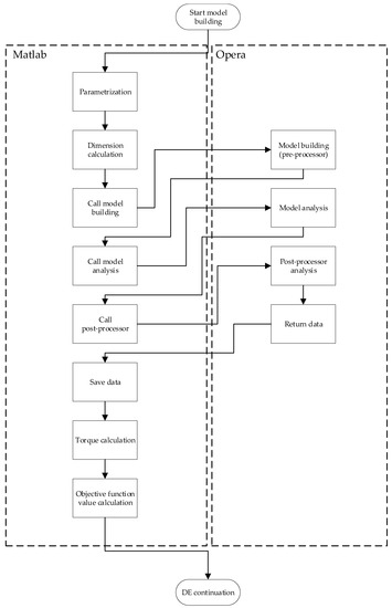
Figure 12. Flowchart of the model building process.

Parallel computing was utilized for model analysis and torque calculations (with the objective function value calculation) for six models simultaneously to speed up the optimization process.

2.2.3. Torque Calculation

The torque of the actuator can be described as a sum of the friction torque, which is always present and is ideally negligible, and field dependent MR torque, which is a combination of the field induced component (change in yield stress) and fluid viscosity-dependent component [25]:

$$T=T_{friction}+T_{MR}.$$

(21)

Friction torque results mainly from the geometry and material selection and was not considered in the optimization process. MR torque is the field dependent torque resulting from the rheological changes of the MR fluid in the external magnetic field. It is calculated as:

$$T_{MR}={{\displaystyle \int }}_S^{ }{r}_{arm}\tau \mathrm{d}A,$$

(22)

where $r_{arm}$ (the lever arm) is the distance of the rotor’s axis of rotation to the small patch $\mathrm{d}A$ on the rotor’s surface, and $\tau$ is the shear stress on that surface. There are two cases: (a) Rotation of the rotor around the vertical axis ($z$ axis), $T_{MR}=T_z$, and (b) Rotation around a horizontal axis (in the plane $xy$), $T_{MR}=T_{xy}$. In case (a), $r_{arm}$ is:

$$r_{arm}=r_r\sin \vartheta ,$$

(23)

where $r_r$ is the rotor radius and $\vartheta$ is the inclination angle. In case (b), $r_{arm}$ is:

$$r_{arm}=r_r\sqrt{{\cos }^2\vartheta +{\sin }^2\vartheta {\sin }^2\phi }.$$

(24)

Here, $\phi$ is the azimuth angle (Figure 2).

Shear stress $\tau$ is the same as the shear stress on the MR fluid in shear mode operation. For a spherical MR actuator application, the shear stress of the MR fluid can be expressed using the Bingham plastic model as used in other publications [6,7,10,11,12,13,14,16,17,25]:

$$\tau ={\tau }_y+{\eta }_B\dot{\gamma },$$

(25)

where ${\tau }_y$ is yield stress, ${\eta }_B$ plastic viscosity, and $\dot{\gamma }$ shear rate. The second term (${\eta }_B\dot{\gamma }$) can be neglected since the rotor’s movements are slow in the actuator’s intended application. The first term (${\tau }_y$) is field dependent. Based on that, Equation (25) can be rewritten as:

$$\tau ={\tau }_y\left(H\right).$$

(26)

For case (a), Equation (22) is rewritten as:

$$T_z={{\displaystyle \int }}_{{\vartheta }_{s1}}^{{\vartheta }_{s2}}{{\displaystyle \int }}_0^{2\pi }\left(r_r\sin \vartheta \right){\tau }_y\left(H\right)r_r^2\sin \vartheta \mathrm{d}\phi \mathrm{d}\vartheta .$$

(27)

For case (b), Equation (22) is rewritten as:

$$T_{xy}={{\displaystyle \int }}_{{\vartheta }_{s1}}^{{\vartheta }_{s2}}{{\displaystyle \int }}_0^{2\pi }\left(r_r\sqrt{{\cos }^2\vartheta +{\sin }^2\vartheta {\sin }^2\phi }\right){\tau }_y\left(H\right)r_r^2\sin \vartheta \mathrm{d}\phi \mathrm{d}\vartheta .$$

(28)

Value ${\vartheta }_{s1}$ is the angle at which the MR fluid starts in the upper part of the actuator (where the rotor, the seal, and the MR fluid meet), and ${\vartheta }_{s2}$ is the angle at which it ends (the lower part of the actuator). From the post-processor, the radial component of magnetic field strength above the surface of the rotor was extracted as a table of $H_{radial}$ values at $\phi$ and $\vartheta$ angles. Since the data were discrete, a numerical approach was used to calculate the previous integrals. The method used for integration was the trapezoidal rule for two variables. Summarized from [26], the trapezoidal rule for two variables ($x$ and $y$) finds the definite integral $I$ as:

$$I={{\displaystyle \sum }}_{i=1}^{N-1}{{\displaystyle \sum }}_{j=1}^{M-1}\frac{\left(x_{i+1}-x_i\right)\left(y_{j+1}-y_j\right)}{4}\left[g\left(x_i,y_j\right)+g\left(x_{i+1},y_j\right)+g\left(x_i,y_{j+1}\right)+g\left(x_{i+1},y_{j+1}\right)\right],$$

(29)

where $i$ and $j$ are the indices of discrete values of $x$ and $y$, respectively, $N$ is the number of values $x$, $M$ is the number of values $y$, and $g$ is the integrated function. Combining integral (27) with Equation (29), with $x\to \vartheta$ and $y\to \phi$, Equation (27) transforms into:

$$T_z={{\displaystyle \sum }}_{i=1}^{N-1}{{\displaystyle \sum }}_{j=1}^{M-1}\frac{\left({\vartheta }_{i+1}-{\vartheta }_i\right)\left({\phi }_{j+1}-{\phi }_j\right)}{4}\left[g_z\left({\vartheta }_i,{\phi }_j\right)+g_z\left({\vartheta }_{i+1},{\phi }_j\right)+g_z\left({\vartheta }_i,{\phi }_{j+1}\right)+g_z\left({\vartheta }_{i+1},{\phi }_{j+1}\right)\right],$$

(30)

where ${\vartheta }_1$ corresponds with ${\vartheta }_{s1}$, ${\vartheta }_N$ with ${\vartheta }_{s2}$, ${\phi }_1$ with 0, and ${\phi }_2$ with 2$\pi$. Function $g_z$ represents the integrating function:

$$g_z\left(\vartheta ,\phi \right)=\left(r_r\sin \vartheta \right){\tau }_y\left(H\right)r_r^2\sin \vartheta .$$

(31)

Similarly, Equation (28) transforms into:

$$T_{xy}={{\displaystyle \sum }}_{i=1}^{N-1}{{\displaystyle \sum }}_{j=1}^{M-1}\frac{\left({\vartheta }_{i+1}-{\vartheta }_i\right)\left({\phi }_{j+1}-{\phi }_j\right)}{4}\left[g_{xy}\left({\vartheta }_i,{\phi }_j\right)+g_{xy}\left({\vartheta }_{i+1},{\phi }_j\right)+g_{xy}\left({\vartheta }_i,{\phi }_{j+1}\right)+g_{xy}\left({\vartheta }_{i+1},{\phi }_{j+1}\right)\right],$$

(32)

with $g_{xy}$ being:

$$g_{xy}\left(\vartheta ,\phi \right)=\left(r_r\sqrt{{\cos }^2\vartheta +{\sin }^2\vartheta {\sin }^2\phi }\right){\tau }_y\left(H\right)r_r^2\sin \vartheta .$$

(33)

The ${\tau }_y\left(H\right)$ curve from Figure 4 was used for the value of ${\tau }_y$ at relevant $H_{radial}$.

2.3. Verification of the Model

A comparison with the results of an analytical approach was made to verify the FEM results. The magnetic field strength $H$ in the gap with MR fluid was approximated using Ampère’s law (Equation (34)) [27]. Ampère’s law was used in the following form:

$$\oint H \mathrm{d}l=NI,$$

(34)

with $\mathrm{d}l$ being the path differential, $N$ the number of coil turns, and $I$ being the current through the coil.

A number of simplifications and assumptions were used:

• Permeability $\mu$ is in a linear regime in the rotor;
• To approximate the apparent permeability in the stator, the value of around $B=$ 1.9 T (based on the FEM prediction in Results—Section 3) was assumed in the stator, and permeability was selected based on Figure 5;
• Similarly, the permeability in the MR fluid gap was selected based on value $B$, around 0.9 T, according to Figure 3;
• The magnetic field in the separate parts (rotor, MR fluid, stator) was assumed to be constant;
• The integral path used was midway between the coil and the edge of the stator;
• The integral path selected for use in Equation (34) is presented in Figure 13.
  

  Figure 13. Path for the integral from Equation (34).

Considering the assumptions, Equation (34) can be rewritten as follows:

$$H_r{l}_r+H_{MR}{l}_{MR}+H_s{l}_s=NI.$$

(35)

Here, $H_r$ is the magnetic field strength of steel in the linear regime, $l_r=2r_r$ is the path in the rotor, $H_s$ is the magnetic field strength of steel in the target field regime, $l_s=2l_{s1}+2l_{s2}+l_{s3}$ is the path in the stator, $H_{MR}$ is the magnetic field strength in the MR fluid, and $l_{MR}=2d_{MR}$ is the path in the MR fluid. $H_r$ and $H_s$ can be represented with $H_{MR}$ and permeabilities as follows:

$$H_r=\frac{{\mu }_{MR}}{{\mu }_r}{H}_{MR},$$

(36)

$$H_s=\frac{{\mu }_{MR}}{{\mu }_s}{H}_{MR},$$

(37)

where ${\mu }_{MR}$, ${\mu }_r$, and ${\mu }_s$ are the relative permeabilities of the MR fluid at the target field, steel in the linear regime, and steel at the target field, respectively. Their values are shown in Table 6.

Table 6. Values of the relative permeabilities used for the analytical calculations.

Relative Permeability	Value
${\mu }_{MR}$	2.7
${\mu }_r$	860
${\mu }_s$	76

Using Equations (35)–(37), the magnetic field strength in the gap with MR fluid can be calculated as:

$$H_{MR}=\frac{NI}{\frac{{\mu }_{MR}}{{\mu }_r}{l}_r+l_{MR}+\frac{{\mu }_{MR}}{{\mu }_s}{l}_s}.$$

(38)

The resulting field was compared to the value of the average radial $H$ from sectors 1 and 2 in Figure 11, obtained from the FEM analysis.

The braking torque was calculated directly using Equations (27) and (28). The torque was calculated above the rotor in the area between the upper and lower seals and not counting the area at the disc, using $H_{MR}$ to evaluate the yield stress ${\tau }_y$ of the MR fluid (Figure 4). According to this, the integrals (27) and (28) were calculated between $\vartheta :$ 45.0238°–83.1629° and 96.8371°–134.9762°.

3. Results

3.1. Reference Model

As stated in Section 2.2.1, first, the reference model was built using the parameter values from Table 4. The resulting reference values, later used in the objective function calculation, are represented in Table 7.

Table 7. Reference values for the objective function calculations.

Parameter	Value
$r_{ar}$	42.5 mm
$h_{ar}$	48.5 mm
$B_{dr}$	0.1901 T
$T_{xyr}$	1.84 Nm
$T_{zr}$	2.3213 Nm

The cross-section of the reference model is shown in Figure 14.

Figure 14. Cross-section of the reference model.

The value of the reference model’s objective function was 0.0082.

3.2. Optimization Results

Although the optimization process was time consuming, it was run three times. The time consumption analysis is presented in Table 8. Relevant information about the computer used is: processor: Intel i7-11700K (3.60 GHz), memory: 32 GB.

Table 8. Time consumption analysis of the optimization process.

	Optimization 1	Optimization 2	Optimization 3
Number of iterations	95	86	63
Reference model building time	7.74 min	7.46 min	7.43 min
Mean iteration time	1.21 h	1.21 h	1.25 h
Mean model creation time	1.19 min	1.17 min	1.19 min
Mean model analysis time	12.25 min	12.39 min	12.94 min
Mean Post-processor analysis time	13.84 s	13.73 s	14.02 s
Mean torque calculation time	0.65 s	0.64 s	0.69 s
Overall time	114.78 h	103.89 h	79.15 h

The resulting dimensions from each optimization process are summarized in Table 9.

Table 9. Resulting dimensions of the actuator parameters.

Parameter	Optimization 1	Optimization 2	Optimization 3
$h_u$	18.5 mm	18.5 mm	18.5 mm
$h_l$	18.5 mm	18.5 mm	18.5 mm
$r_a$	43.6851 mm	44.1522 mm	43.7460 mm
$d_d$	5 mm	5 mm	5 mm

Since the outermost part of the seal was above the coil at the top (and below at the bottom), the inner radius of the coil was calculated using Equation (13).

As seen from Table 9, both the upper and lower dimensions gravitated towards the lower bound value while the disc thickness gravitated towards the upper bound value. The parameter $r_a$ is somewhere between the lower and upper boundaries. Even though the resulting radii were different (43.6851 mm, 44.1522 mm, and 43.7460 mm), it was later shown that the objective function value changed minimally in the region around the minimum.

The values used for calculating the objective functions obtained from the post-processor and torque calculation for the optimal model are shown in Table 10.

Table 10. Values used in the objective function (Equations (16)–(19)) for the optimal model.

Parameter	Optimization 1	Optimization 2	Optimization 3
$B_d$	0.0750 T	0.0759 T	0.0752 T
$B_1$	0.9278 T	0.9328 T	0.9283 T
$B_2$	0.9276 T	0.9327 T	0.9285 T
$B_3$	1.8962 T	1.9091 T	1.9018 T
$B_4$	1.8997 T	1.9060 T	1.9005 T
$B_5$	1.9008 T	1.9114 T	1.9027 T
$T_{xy}$	2.8996 Nm	2.9162 Nm	2.9019 Nm
$T_z$	3.3212 Nm	3.3403 Nm	3.3239 Nm
Objective Function: $f$	−0.3362	−0.3362	−0.3361

How the objective function value of the best population member changed through the generations is shown in Figure 15.

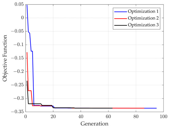
Figure 15. Objective function value of the best population member through the generations.

Figure 16 shows how the parameters changed through the generations.

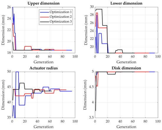
Figure 16. Change in parameters through the generations.

Figure 17 shows the objective function dependence on the actuator radius $r_a$ at fixed values of the upper dimension $h_u$ = 18.5 mm, lower dimension $h_l$ = 18.5, and disc thickness $d_d$ = 5 mm.

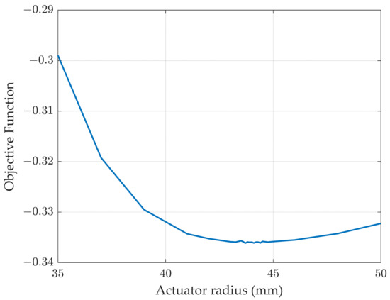
Figure 17. Objective function dependency on the actuator radius at fixed values of $h_u$ = 18.5 mm, $h_l$ = 18.5 mm, and $d_d$ = 5 mm.

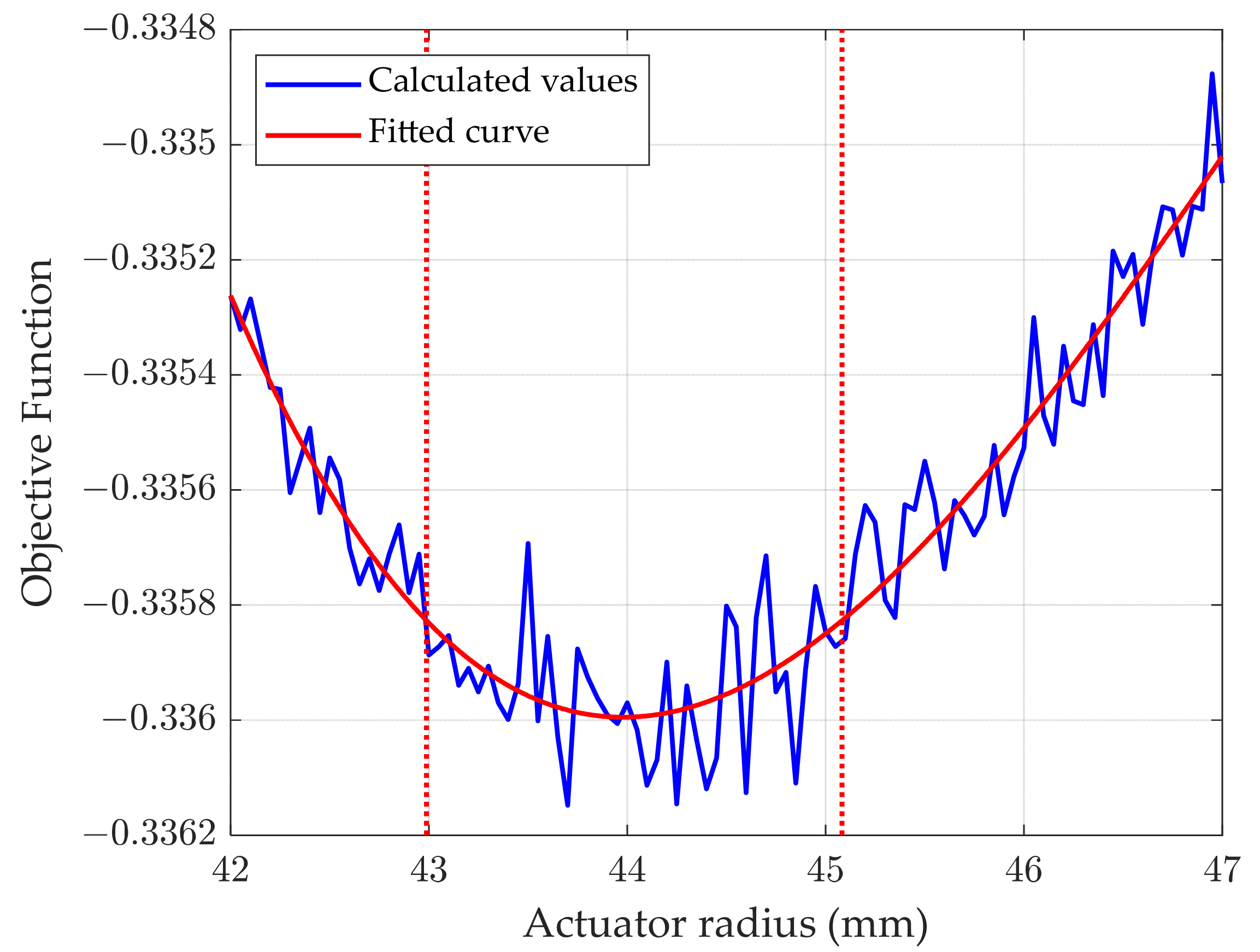
Figure 18 shows a zoomed in curve from Figure 17 at the minimum values of the objective function (between $r_a$ = 42 mm and $r_a$ = 47 mm). Because of the scale selection of the y-axis (Objective Function), there appears to be much variation in the calculation results presented in Figure 18. This is due to minor differences in mesh creation in the FEM modeling. The calculated dependency in Figure 18 was fitted with a third-degree polynomial using the least squares method for analysis. The range in which the minimum is found was defined with values of the $r_a$, between which the fitted curve changed less than 0.05% compared to the fitted curve’s minimum value. The resulting range was between $r_a$ = 42.9880 mm and $r_a$ = 45.0831 mm, represented by the two vertical dotted lines in Figure 18. The relative difference between the upper and lower values of $r_a$, in regard to the lower value, was 4.87%.

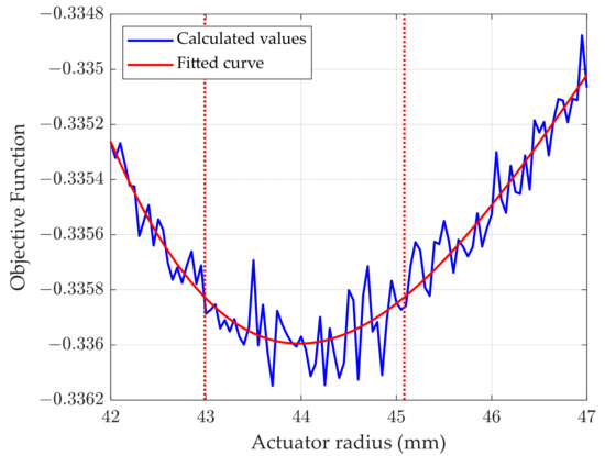
Figure 18. Objective function dependency on the actuator radius between $r_a$ = 42 mm and $r_a$ = 47 mm. The calculated values were fitted with a third-degree polynomial using the least squares method. The dotted vertical lines represent the lower and upper values between which the minimum of the objective function was found.

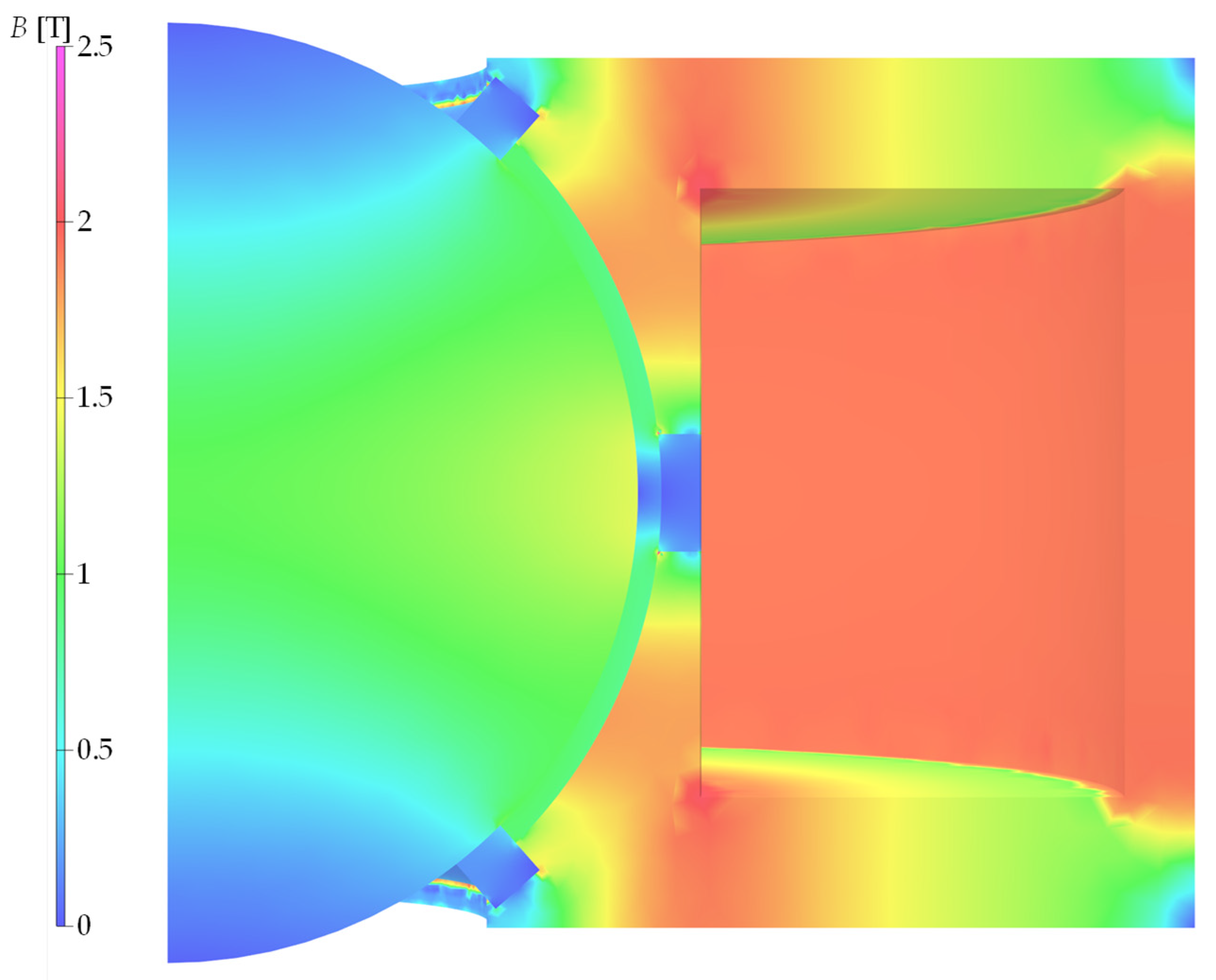
Figure 19 shows the magnetic flux density distribution at maximum load ($j=$ 3.2 A/mm²) for the optimum model (optimization 1).

Figure 19. Magnetic flux density distribution in the actuator model (optimization 1).

3.3. Model Verification Results

The analytical calculations for the FEM verification were performed for the optimized models’ geometric and coil current data. In this section, example 1, example 2, and example 3 correspond with optimized models 1, 2, and 3, respectively. The lengths of the paths and values $NI$ used in Equation (38) are presented in Table 11 for example 1, Table 12 for example 2, and Table 13 for example 3.

Table 11. Path lengths and $NI$ value used for calculation in example 1.

Parameter	Value
$l_{s1}$	6.5671 mm
$l_{s2}$	19.5541 mm
$l_{s3}$	31.4504 mm
$NI$	1469.2716 A

Table 12. Path lengths and $NI$ value used for calculation in example 2.

Parameter	Value
$l_{s1}$	6.5671 mm
$l_{s2}$	20.0380 mm
$l_{s3}$	31.4504 mm
$NI$	1510.4669 A

Table 13. Path lengths and $NI$ value used for calculation in example 3.

Parameter	Value
$l_{s1}$	6.5671 mm
$l_{s2}$	19.6172 mm
$l_{s3}$	31.4504 mm
$NI$	1474.6502 A

The resulting magnetic field strength values in the MR fluid gap $H_{MR}$ and comparisons to the FEM results are presented in Table 14. The relative deviation was calculated using the following:

$$\Delta H_{rel}=\frac{\left|H_{MR}\left(analytical\right)-H_{MR}\left(FEM\right)\right|}{H_{MR}\left(FEM\right)}.$$

(39)

Table 14. $H_{MR}$ values calculated for each example and compared to the FEM results.

Example	Analytical ${\mathit{H}}_{\mathit{M}\mathit{R}}$ (kA/m)	FEM ${\mathit{H}}_{\mathit{M}\mathit{R}}$ (kA/m)	$\mathbf{\Delta }{\mathit{H}}_{\mathit{r}\mathit{e}\mathit{l}}$ (%)
1	288.1559	235.9308	22.1358
2	294.2506	238.9515	23.1424
3	288.9565	236.3426	22.2617

Using the analytical values of $H_{MR}$, the braking torque was calculated using Equations (27) and (28). The results are shown in Table 15. The relative deviation of the torque was calculated using:

$$\Delta T_{rel}=\frac{\left|T\left(analytical\right)-T\left(FEM\right)\right|}{T\left(FEM\right)}.$$

(40)

Table 15. Calculated torque values for each of the examples and comparison to the FEM results.

Example	Analytical Torque	FEM Torque	$\mathbf{\Delta }{\mathit{T}}_{\mathit{r}\mathit{e}\mathit{l}}$ (%)
1	$T_z=$ 3.5758 Nm	$T_z=$ 3.3212 Nm	7.6659
	$T_{xy}=$ 2.9806 Nm	$T_{xy}=$ 2.8996 Nm	2.7935
2	$T_z=$ 3.6079 Nm	$T_z=$ 3.3403 Nm	8.0113
	$T_{xy}=$ 3.0074 Nm	$T_{xy}=$ 2.9162 Nm	3.1274
3	$T_z=$ 3.5800 Nm	$T_z=$ 3.3239 Nm	7.7048
	$T_{xy}=$ 2.9842 Nm	$T_{xy}=$ 2.9019 Nm	2.8361

As seen from Table 14 and Table 15, the relative differences in the magnetic field strength in the MR fluid gap were around 22% and 23% while the differences in torque were around 8% for $T_z$ and 3% for $T_{xy}$. The FEM calculations are verified with these results.

4. Conclusions

A suitable FEM model of the spherical MR actuator was built and linked to the DE optimization algorithm with the help of model parameterization. This enabled an automated optimization process. Despite the random manipulation of the four parameters (Table 3), the DE algorithm and FEM model building ran fluently.

Much consideration was placed on the selection of the objectives of the objective function. In the end, torque, size, and magnetic flux density in the actuator were selected as the objective function criteria. Priority was given to the actuator’s torque capabilities, with size being the second most important. The least important was the magnetic flux density. The objective function was defined as a combination of weighted and normalized differences between the relevant calculated quantities and the desired (absolute differences) or reference values (constructed so that the algorithm searches for the minimum or maximum value) of the said quantities. The reference values were calculated using the midpoint values between the lower and upper bound values of the four parameters (Table 3) being optimized in the optimization process. Such an approach was not found in other publications. It is a helpful approach, especially when the values are unknown. Therefore, it is also recommended for use in other types of electromagnetic device development.

DE was used successfully for the design optimization of the spherical MR actuator. The algorithm searched for the values of four parameters using a multi-objective objective function (Equations (16)–(19)). FEM was utilized to create and analyze each model in the optimization algorithm. Three independent passes of the optimization process were performed, with similar results. In each pass, parameters $h_u$ and $h_l$ gravitated towards the lower boundary value, $d_d$ towards the upper boundary value, and the actuator radius $r_a$ occupied a value between 42.9880 mm and 45.0831 mm, which is about a 5% difference regarding the lower value. These results prove that the optimization process is robust, and that the objective function selection was appropriate.

The whole process was time consuming. Three passes of the optimization were performed, individually taking about 114.78 h, 103.89 h, and 79.15 h to finish. Together, that is 297.82 h, or approximately 12.41 days. This time could be shortened by using more powerful equipment and a more optimized algorithm code.

From the actuator design point of view, a suitable geometry parametrization was introduced to build a basic model given the parameters from Table 2 and Table 3. After optimization, three of the four parameters to be optimized, namely upper dimension, lower dimension, and disc thickness, were pinned to a fixed value: $h_u=$ 18.5 mm, $h_l=$ 18.5 mm, and $d_d=$ 5 mm. The fourth parameter, actuator radius $r_a$, fell between 42.9880 mm and 45.0831 mm. It makes sense to select a value in this range. For instance, the midpoint value of $r_a=$ 44.0356 mm. This makes the model wholly defined geometrically. With this, the best ratio between braking torque and actuator size was achieved within the constraints. Although the approach is shown in a concrete example, it gives others a framework for optimizing a similar device and forming an appropriate objective function.

A comparison between the FEM results and the results obtained via an analytical approach was made to verify the FEM calculations. In the analytical approach, the braking torque was calculated using the magnetic field strength in the MR fluid obtained using Ampère’s law. The analytical approach gave $H_{MR}$ values that were around 23% higher than the FEM results, and torque values that were 8% and 3% higher for $T_z$ and $T_{xy}$, respectively. The FEM calculations were verified with these results. It should be noted that, while the results are similar, several assumptions were made in the analytical approach. The major assumption was that the magnetic field was constant in different actuator parts. The relative permeability was then selected for each part as a constant value based on the expected field values. The selection of the correct permeabilities is crucial since the resulting field in the MR fluid gap depends significantly on their values. It is also difficult since a small change in the expected magnetic field can lead to a significant change in permeability value. These shortcomings are avoided by using the FEM approach. The FEM approach takes into account the non-linearity of the materials. It calculates the magnetic field that changes from point to point in a given region, giving more accurate and detailed results. Therefore, while an analytical approach gives good enough results to validate the results of the FEM approach, given that the permeabilities and magnetic fields selected are close to actual values, the results are not accurate enough to be used as the main approach to the design.

In future work, the focus will be on building a prototype of the actuator, measuring the torque characteristics, and comparing them to the model’s. Regarding the optimization process, steps will be taken to speed up the process, allowing for quicker optimization of devices and more passes to be performed in a reasonable amount of time.

References

- Vizjak, J.; Beković, M.; Jesenik, M.; Hamler, A. Development of a Magnetic Fluid Heating FEM Simulation Model with Coupled Steady State Magnetic and Transient Thermal Calculation. Mathematics 2021, 9, 2561. [Google Scholar] [CrossRef]
- Kuznetsov, N.M.; Kovaleva, V.V.; Belousov, S.I.; Chvalun, S.N. Electrorheological Fluids: From Historical Retrospective to Recent Trends. Mater. Today Chem. 2022, 26, 101066. [Google Scholar] [CrossRef]
- Eshgarf, H.; Ahmadi Nadooshan, A.; Raisi, A. An Overview on Properties and Applications of Magnetorheological Fluids: Dampers, Batteries, Valves and Brakes. J. Energy Storage 2022, 50, 104648. [Google Scholar] [CrossRef]
- Hajalilou, A.; Amri Mazlan, S.; Lavvafi, H.; Shameli, K. Magnetorheological (MR) Fluids. In Field Responsive Fluids as Smart Materials; Hajalilou, A., Amri Mazlan, S., Lavvafi, H., Shameli, K., Eds.; Springer: Singapore, 2016; pp. 13–50. ISBN 978-981-10-2495-5. [Google Scholar]
- Rabinow, J. The Magnetic Fluid Clutch. Electr. Eng. 1948, 67, 1167. [Google Scholar] [CrossRef]
- Chen, D.; Song, A.; Tian, L.; Ouyang, Q.; Xiong, P. Development of a Multidirectional Controlled Small-Scale Spherical MR Actuator for Haptic Applications. IEEE/ASME Trans. Mechatron. 2019, 24, 1597–1607. [Google Scholar] [CrossRef]
- Senkal, D.; Gurocak, H. Spherical Brake with MR Fluid as Multi Degree of Freedom Actuator for Haptics. J. Intell. Mater. Syst. Struct. 2009, 20, 2149–2160. [Google Scholar] [CrossRef]
- Ghavghave, M.; Darade, P.D. Spherical Smart Brake for Multi-Degree of Freedom and Positional Stability. Mater. Today Proc. 2017, 4, 7793–7800. [Google Scholar] [CrossRef]
- Zhou, G.; Gurocak, H. Spherical Magnetorheological Brake with Optical Mouse Sensors. In Proceedings of the 2021 9th International Conference on Control, Mechatronics and Automation (ICCMA), Belval, Luxembourg, 11 November 2021; pp. 165–170. [Google Scholar]
- Karakoc, K.; Park, E.J.; Suleman, A. Design Considerations for an Automotive Magnetorheological Brake. Mechatronics 2008, 18, 434–447. [Google Scholar] [CrossRef]
- Park, E.J.; Stoikov, D.; Falcao da Luz, L.; Suleman, A. A Performance Evaluation of an Automotive Magnetorheological Brake Design with a Sliding Mode Controller. Mechatronics 2006, 16, 405–416. [Google Scholar] [CrossRef]
- Assadsangabi, B.; Daneshmand, F.; Vahdati, N.; Eghtesad, M.; Bazargan-Lari, Y. Optimization and Design of Disk-Type MR Brakes. Int. J. Automot. Technol. 2011, 12, 921–932. [Google Scholar] [CrossRef]
- Hajiyan, M.; Mahmud, S.; Biglarbegian, M.; Abdullah, H.A. A New Design of Magnetorheological Fluid Based Braking System Using Genetic Algorithm Optimization. Int. J. Mech. Mater. Des. 2016, 12, 449–462. [Google Scholar] [CrossRef]
- Topcu, O.; Taşcıoğlu, Y.; Konukseven, E.İ. Design and Multi-Physics Optimization of Rotary MRF Brakes. Results Phys. 2018, 8, 805–818. [Google Scholar] [CrossRef]
- Shamieh, H.; Sedaghati, R. Development, Optimization, and Control of a Novel Magnetorheological Brake with No Zero-Field Viscous Torque for Automotive Applications. J. Intell. Mater. Syst. Struct. 2018, 29, 3199–3213. [Google Scholar] [CrossRef]
- Senkal, D.; Gurocak, H. Serpentine Flux Path for High Torque MRF Brakes in Haptics Applications. Mechatronics 2010, 20, 377–383. [Google Scholar] [CrossRef]
- Acharya, S.; Saini, T.R.S.; Sundaram, V.; Kumar, H. Selection of Optimal Composition of MR Fluid for a Brake Designed Using MOGA Optimization Coupled with Magnetic FEA Analysis. J. Intell. Mater. Syst. Struct. 2021, 32, 1831–1854. [Google Scholar] [CrossRef]
- Bucchi, F.; Forte, P.; Frendo, F. Geometry Optimization of a Magnetorheological Clutch Operated by Coils. Proc. Inst. Mech. Eng. Part L J. Mater. Des. Appl. 2017, 231, 100–112. [Google Scholar] [CrossRef]
- Erol, O.; Gurocak, H. Mr-Brake with Permanent Magnet as Passive Actuator for Haptics. In Proceedings of the 2013 World Haptics Conference (WHC), Daejeon, Republic of Korea, 14 April 2013; pp. 413–418. [Google Scholar]
- Nguyen, H.; Choi, S. Optimal Design of a T-Shaped Drum-Type Brake for Motorcycle Utilizing Magnetorheological Fluid. Mech. Based Des. Struct. Mach. 2012, 40, 153–162. [Google Scholar] [CrossRef]
- Price, K.; Storn, R.; Lampinen, J. Differential Evolution—A Practical Approach to Global Optimization; Springer Science & Business Media: Berlin/Heidelberg, Germany, 2005; Volume 141. [Google Scholar]
- Jesenik, M.; Mernik, M.; Trlep, M. Determination of a Hysteresis Model Parameters with the Use of Different Evolutionary Methods for an Innovative Hysteresis Model. Mathematics 2020, 8, 201. [Google Scholar] [CrossRef]
- Jesenik, M.; Hamler, A.; Trbušić, M.; Trlep, M. The Use of Evolutionary Methods for the Determination of a DC Motor and Drive Parameters Based on the Current and Angular Speed Response. Mathematics 2020, 8, 1269. [Google Scholar] [CrossRef]
- Arus MR Tech. Magnaflo. Available online: https://arusmrtech.com/wp-content/uploads/2021/11/MAGNAFLO.pdf (accessed on 15 August 2023).
- Poznić, A.; Zelić, A.; Szabó, L. Magnetorheological Fluid Brake–Basic Performances Testing with Magnetic Field Efficiency Improvement Proposal. Hung. J. Ind. Chem. 2012, 40, 107–111. [Google Scholar]
- Dhali, M.; Hasan, M.; Selim, A.; Barman, N. Numerical Double Integration for Unequal Data Spaces. Int. J. Math. Sci. Comput. 2020, 6, 24–29. [Google Scholar] [CrossRef]
- Griffiths, D.J. Introduction to Electrodynamics, 4th ed.; Cambridge University Press: Cambridge, UK, 2017. [Google Scholar]
Disclaimer/Publisher’s Note: The statements, opinions and data contained in all publications are solely those of the individual author(s) and contributor(s) and not of MDPI and/or the editor(s). MDPI and/or the editor(s) disclaim responsibility for any injury to people or property resulting from any ideas, methods, instructions or products referred to in the content. |
© 2023 by the authors. Licensee MDPI, Basel, Switzerland. This article is an open access article distributed under the terms and conditions of the Creative Commons Attribution (CC BY) license (https://creativecommons.org/licenses/by/4.0/).