Abstract
Structural Health Monitoring (SHM) techniques, such as Electromechanical Impedance Spectroscopy (EMIS), aim to continuously monitor structures for defects, thus avoiding the need for regular maintenance. While attention has been given to the application of EMIS in the automatic detection of damage in metallic and composite components, integrity monitoring of structural adhesive joints has been comparatively neglected. This paper investigated the use of damage metrics with electrical impedance measurements to detect defects in Single-Lap Joints (SLJs) bonded with a modified epoxy adhesive. Traditional metrics using statistical and distance-based concepts, such as the Root-Mean-Squared Deviation, , or the Correlation Coefficient, , are addressed at detecting voids in the adhesive layer and are applied to five different spectral frequency ranges. Furthermore, new damage metrics have been developed, such as the Average Canberra Distance, , which enables a reduction of possible outliers in damage detection, or the complex Root-Mean-Squared Deviation, , which allows for the use of both the real and imaginary components of the impedance, enabling better damage detection in structural adhesive joints. Overall, damage detection is achieved, and for certain spectral conditions, differentiation between certain damage sizes, using specific metrics, such as the or , may be possible. Overall, the or values from damaged SLJs tend to be double the metric values from undamaged joints.
Keywords:
structural health monitoring; electromechanical impedance spectroscopy; adhesive joints; damage metrics; piezoelectric sensors; void MSC:
68M18
1. Introduction
Structural Health Monitoring (SHM) is the scientific and engineering domain of automatic and continuous inspection of damage in structures. In this manner, sensors are placed in a given structure and measure dynamic physical quantities that are influenced by material and structural properties. If damage is present, these properties will vary, and therefore, the dynamic behavior being measured will also change. Given this, a computer will acquire these measurements and input them into algorithms for damage detection and evaluation [1,2]. The use of SHM may reduce the number of out-of-service operations and possibly eliminate the need for alternative tools for damage detection, namely Non-Destructive Testing (NDT) [2,3].
Various integrity-monitoring techniques exist, some of which are based on the coupled electromechanical behavior of Piezoelectric Wafer Active Sensors (PWAS) [1,2,4,5,6]. One such method is the Electromechanical Impedance Spectroscopy (EMIS) monitoring technique, where a PWAS is supplied by an AC voltage source, with a sweep of the signal frequency, , across a range of values, normally above 1 kHz. In this manner, for each frequency, , the PWAS will convert the voltage signal, , into a mechanical force, , and particle velocity, . Concurrently, the stress–strain vibrations influence the electrical current, . Consequently, the PWAS behaves simultaneously as a vibration actuator and sensor, but the associated mechanical variables, and , are indirectly measured, given that an impedance analyzer captures the electrical impedance of the PWAS for the examined frequency spectrum, [6].
Various studies have proposed mathematical models relating the mechanical load and velocity, and , respectively, or the mechanical impedance of the structure, , with the electrical impedance measurements [7,8,9,10,11]. One such model, formulated by Liang et al. [7], correlates the electrical impedance with the impedance of a one-dimensional structure with concentrated mass, , stiffness, , and damping, , like the one in Figure 1, yielding
where the width, length, and thickness of the piezoelectric element are , , and , respectively. The variable stands for the mechanical impedance of the PWAS, while j and correspond to the imaginary number, , and the piezoelectric-induced strain coefficient, respectively. The complex Young’s Modulus of the PWAS material with a null electric filed (), , is defined as , where is the mechanical loss factor, and the dielectric constant at zero stress, , is expressed as , where is the dielectric loss factor. It is noted that, in these models, structural damping and stiffness are considered constant throughout the inspection frequency range, which may not always be true, as shown in [12].
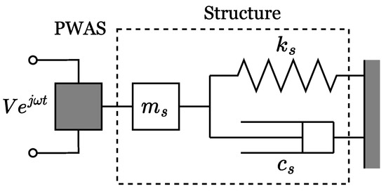
Figure 1.
Model of interaction between the PWAS and a one-dimensional structure that occurs in the EMIS method, proposed by Liang et al. [7].
One should consider that the impedance of the sensor, , has real and imaginary components, corresponding, respectively, to the resistive and reactance elements of an equivalent electrical circuit. However, the imaginary component is mainly dominated by the dielectric constant , which is passive in the sense that it is independent of the structural parameters, i.e., mechanical impedance, . In mathematical terms,
where is the electrical admittance, which is the inverse of the electrical impedance. This admittance can be decomposed into a passive and active admittance, and , respectively.
From this formulation, one can deduce that the passive component, , corresponds to the electrical admittance of a parallel plate capacitor and consists of a complex vector mainly contributing to the reactance [13]. In this manner, the active component is the main contributor to the real component of the measured electrical impedance, which is more sensitive to damage, as shown by Bhalla et al. [14].
Research on NDT methods, to examine the bondline integrity of structural adhesive joints, has been considerably small in nature and scope [5,6,15,16,17,18], especially given the widespread use of structural adhesives in vehicular structures [19,20,21,22,23], e.g., airplanes, automobiles, boats, etc. Indeed, recent studies on NDT inspection of adhesive joints show that not all types of adhesive defects are detectable, requiring the combined use of various NDT techniques, complex signal processing tools, and expensive testing apparatuses [24,25,26,27,28]. In this manner, SHM methods, such as EMIS, can gain scientific and industrial relevance for damage detection.
One manner of evaluating if a given SHM method is able to detect a given form of damage in a type of structure or material is to compare measurements between damaged and undamaged structures. This is performed with the help of damage metrics, given that they have a simple computation, and for the specific case of EMIS, these make use of the real component of the measured electrical impedance, . Some metrics are adopted in this field, such as the Mean Absolute Percentage Deviation, , or Pearson’s Correlation Coefficient, . However, the most-widely adopted damage metric is the Root-Mean-Squared Deviation, , and for the specific case of adhesive joint integrity monitoring, this is the only damage index being used in scientific research [6].
Na, Tawie, and Lee [29] studied the detectability of adhesive mass loss in glass-fiber-reinforced polymer adhesive joints, after immersion in acetone, which is considered a corrosive solution. Damage could be detected by computing the Root-Mean-Squared Deviation damage metric, , which is defined as
where and are the real impedance components of the signal under evaluation and of a reference/pristine measurement, respectively. Note also that and stand, respectively, for the initial and final sampled angular frequencies of both measurements. These frequencies are related to the initial and final frequency variables, and , respectively, such that . Malinowski et al. [30] used a combination of both the and the peak frequency shift as dimensional metrics to detect damage in Single-Lap Joints (SLJs). Damage was created using either pockets of uncured adhesive (by reducing the curing cycle), release agent contamination, or moisture contamination. For both the joints with release agent contamination and damage caused by moisture, only the values changed. However, when analyzing measurements from joints with pockets of uncured adhesive, a decrease of both metrics occurred.
Roth and Girgiutiu [31] evaluated the sensitivity of EMIS to detect voids in adhesive joints. To achieve this, an initial finite element modal analysis determined the best mode shapes for damage detection, and posteriorly, a second simulation yielded the optimal PWAS placement for intact and debonded joints.
Zhuang et al. [32] performed cyclic load testing, with increasing load steps, on epoxy SLJ specimens with artificially created weak adhesion (also known as kissing bond). Between each load cycle, PWAS impedance was measured and the damage metric was computed. In an initial stage, the damage metric remained unchanged, until reaching a threshold value of 0.2, where one would reach approximately 80% of the specimen’s failure stress. Malinowski et al. [33] correlated the mechanical performance of adhesive joints with electrical impedance measurements and verified that the spectra from 4.25 to 4.7 MHz changed according to the bond quality of the adhesive joint. The authors also verified that the values were in agreement with Mode I and Mode II fracture-toughness values.
This paper evaluated EMIS’s capability to monitor the integrity of aluminum adhesive joints, whose electrical measurements were studied in [34]. This was performed by computing damage metrics that made use of both the measured electrical impedance, as well as the active impedance. In this manner, the different metrics may have differing results, which may improve the performance of damage detection, depending on the type of damage and on the type of structure. When using the measurements directly, only the real component of the electrical impedance, Re(), was used in damage detection. In this case, the Root-Mean-Squared Deviation, , the modified Root-Mean-Squared Deviation, , the Mean Absolute Percentage Deviation, , and the Correlation Coefficient, , were used as traditional EMIS damage metrics. Furthermore, a new damage index—the Average Canberra Distance, —is also proposed and tested, enabling a reduction of outliers in damage detection. Conversely, new damage metrics are also proposed that make use of the active electrical impedance, thus including both the real and imaginary components, Re() and Im(), respectively. These metrics include the complex Root-Mean-Squared Deviation, , the Complex Correlation Coefficient, , and the Normalized Complex Euclidean Distance, .
In this manner, Section 2 presents and defines the aforementioned damage metrics, while Section 3 describes the manufacturing and instrumentation of the SLJ specimens, as well as the measurement procedure and spectral conditions for this investigation. Section 4 presents and discusses the obtained results on the application of these metrics for void detection in adhesive joints. Finally, Section 5 presents the concluding remarks of this research.
2. Damage Metrics
Various damage metrics have been proposed for EMIS-based damage detection. However, while studying the viability of EMIS-based integrity evaluation of adhesive joints, the Root-Mean-Squared Deviation metric, , appears to be the only defect metric adopted. In this manner, the most-commonly used EMIS damage metric indices are listed here, as well as the proposed alternatives that make use of the real component of the measured impedance, Re().
Furthermore, it is known that the measured impedance contains a passive component (different from the complex rectangular coordinate impedance components), which is insensitive to damage and is mainly observed in the imaginary component, . However, to the best of the authors’ knowledge, no previous work has been performed where this passive impedance component is removed for damage detection. In this manner, new damage metrics are proposed, where the passive component has been removed.
2.1. Conventional Damage Metrics
While the damage metric, as presented in Equation (4), normally correlates well with damage present in adhesive joints, it has so far been the main metric used to evaluate the applicability of EMIS in defect detection of adhesive joints. Note that this metric can be viewed as a normalized Euclidean norm, [35,36].
However, other metrics have also been employed in comparing impedance spectra to determine the presence of damage [6], such as the Mean Absolute Percentage Deviation, , and the Correlation Coefficient, , which are defined as
where N is the number of acquired samples. Furthermore, the variables and stand for, respectively, the mean value of the measured electric impedance from both the reference pristine joint and the joint under evaluation, while and are the standard deviation of both aforementioned impedances [6].
The Mean Absolute Percentage Deviation, , is a metric that averages the deviations of at all sampled frequencies [35]. However, given its mathematical formulation, this metric can also be viewed as an averaged and normalized Manhattan distance ( distance) damage index, which makes use of the real component of the measured impedance [36].
The Correlation Coefficient, , is based on the Covariance, , and therefore, the authors chose to only include the metric in this investigation [6]. The Covariance, Cov, evaluates the relationship between two impedance signatures and determines whether these two impedance datasets resemble each other or not. If both signatures peak at the same frequency, then the covariance is positive. Conversely, if the peak of a dataset is placed where the valley of the other dataset is, then the covariance is negative. If both signatures are unrelated, then the covariance tends to be null. The CC reflects the same information as the covariance, but the value is normalized so that CC nears 1 when both signatures are similar and is equal to 1 when they are opposite each other [6,37].
While these are the main damage indices used in EMIS, others do exist. One such example is the modified Root-Mean-Squared Deviation damage metric, , which is defined as
and is usually misidentified as the [38,39]. Indeed, this modified metric is equivalent to the , despite the fact that no averaging is performed, since the summation is not divided by the number of sampled frequencies, N, converse to what occurs in Equation (5). Therefore, this damage metric pertains to the family of metrics inspired by the Euclidean distance, , corresponding to the Pearson divergence [40].
2.2. Proposed Damage Metrics
In this work, new damage metrics are also proposed, to try and obtain other methods of damage detection. One proposed metric is the Averaged Canberra Distance, , which is defined as
This metric is based on the Canberra distance, which is used in data quantification, especially for data that are scattered near zero, given that it is sensitive to small values [40,41].
Given the considerations of Bhalla et al. [14], regarding the usefulness of using the active component of the measured impedance, the passive component was removed, which is defined in Equation (3a), yielding only the active component, which, in this paper, is identified by the notation .
A complex Root-Mean-Squared Deviation index, , is proposed as an extension of the classical damage metric and is defined as
which, in simple terms, is the sum of two individual metrics, where one uses the real components of the active impedance from the evaluated and pristine SLJs, and , respectively, and the second part is computed with the imaginary component of said impedances, and .
A modification of the correlation coefficient is proposed to encompass the real and imaginary components of the active impedance, . This complex Correlation Coefficient, , is defined as
which can be viewed as the sum of two individual correlation coefficients, one that only compares the real component of the impedance signals and another that compares the imaginary impedance component. In this manner, the standard deviations of the real and imaginary components of the active electrical impedance of the pristine joint, and , respectively, as well as of the bonded joint under evaluation and , respectively, must be computed. Note that the summed components yield a value between and 2. Therefore, to have an accurate comparison with the traditional metric defined in Equation (6), the resultant summation was divided by 2.
A third proposed metric that makes use of both the active resistance and reactance of the PWAS is the Normalized Complex Euclidean Distance, , such that
This damage index is an alternative proposal of a Euclidean-based damage metric. For this index, the normalization was performed with the complex active impedance of the damageless adhesive joint.
3. Experimental Details
This section presents the specimen materials, their manufacturing procedure, and their measurement conditions. It is noted that this work used the specimens manufactured and studied in [34]. In this manner, the production of the specimens will be briefly described here.
3.1. Materials and Manufacture
The SLJ specimens were manufactured with 6082 aluminum alloy adherends of a 2 mm thickness. The adhesive for SLJ production was the Nagase T-836/R-810 crash-resistant adhesive, which is a modified epoxy adhesive specially conceived of for automobile and aeronautical structures and is manufactured by Nagase ChemteX® (Osaka, Japan). This adhesive cures at a temperature of 160 C for 3 h. The properties of both materials are presented in Table 1.

Table 1.
Properties of the adhesives and adherend used in SLJ manufacturing [12].
The substrates were initially roughened with sand paper. Anodization was performed, as per the standard ASTM D 393398 [42], where the aluminum substrates were submerged in a solution of 10% phosphoric acid and 90% distilled water (m/m), and a current, created by a 16 V voltage, passed through the substrates for 25 min. Afterwards, the substrates were rinsed with distilled water and acetone.
For void creation, Polytetrafluoroethylene (PTFE) infills were placed in the overlap region, before applying the structural crash-resistant adhesive. Subsequently, the mold, with the SLJs, was placed in a hot press, where the aforementioned curing cycle was performed. Note that the infills of diameters mm were placed in either the corner or the center of the overlap layer, as per Figure 2, with the help of a cyanoacrilate adhesive capable of withstanding high temperatures (C).
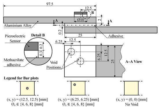
Figure 2.
Schematic representation of an SLJ specimen (with dimensions in mm).
After the manufacture of these adhesive joint specimens, the authors observed that a second source of damage was unintentionally created, as stated in [34]. In this manner, the actual void present in the adhesive layer was constituted by the infill material and a region surrounding this infill, which was unintentionally created. The authors believe that this second source of defect was caused by an unwanted chemical reaction between the modified epoxy adhesive and the cyanoacrilate adhesive. Nonetheless, the main damage to be detected should be the circular void, given that it defines the majority of the damaged area in the overlap.
3.2. Specimen Instrumentation and Measurements
After the manufacturing of the SLJ specimens, PRYY + 1119 piezoelectric sensors, fabricated by PI Ceramics (Lederhose, Germany), were used to instrument said joints. These elements, whose dimensions are indicated in Figure 2, are made of PIC 255 piezoceramic, which has a high Curie temperature ( = 350 C) and whose material properties are presented in Table 2. Note that is the mass density of the piezoceramic, while is the relative permittivity in the polarization direction. The PWAS was fixed on the free side of the upper substrate, in the center of the overlap, with the help of a manually mixed methacrylate adhesive Plexus MA 422, manufactured by ITW Performance Polymers (Chicago, IL, USA), which cures at room temperature for 24 h. The mechanical properties of this adhesive are present in Table 3. Before this cure, a spiral copper wire was placed under the piezoelectric element, and afterwards, a second wire was soldered on top of said element.
Table 2.
Properties of the soft piezoceramic material PIC 255.
Table 3.
Properties of the adhesive used in the SLJ instrumentation [12].
Impedance measurements were performed with a Hioki IM 3570 impedance analyzer (Ueda, Japan), where the adhesive joints were fixed on both free ends with clamps, as demonstrated in Figure 3. This was performed since the boundary conditions influence the measured electrical impedance, . Three impedance spectra were directly measured for each specimen: (i) from kHz to MHz, with linearly spaced sampled frequencies, (ii) from kHz to MHz, with logarithmically spaced frequencies, and (iii) from kHz to MHz, with linearly spaced sampled frequencies. Each measurement yielded 801 sampled frequency points. A plot of the measurements is given in Figure 4.
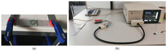
Figure 3.
Experimental setup. (a) Fixed adhesive joint specimen. (b) Impedance analyzer with SLJ.
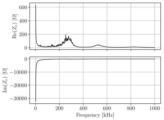
Figure 4.
Plot showing the measured electrical impedance from an undamaged SLJ, with 801 linearly spaced points, from kHz to MHz.
These measurements were then processed by a Python 3 script that computes the damage metrics for each spectral condition. During this processing, two other spectra were created: (iv) the three spectra were combined to yield a spectrum from kHz to MHz with 2389 sampled points; (v) a sub-spectrum was also created from the experimentally obtained spectrum (ii), containing all sampled points between kHz to kHz. Note that, for Spectra (iv), all repeated sampled frequencies were removed.
The aforementioned damage metrics were calculated for all SLJs. However, this required a pristine/reference measurement. In this manner, each pristine SLJ impedance measurement was used as a reference, and all other measurements from all other damaged and damageless joints were considered as measurements from joints under inspection. Therefore, for each reference joint, a total of 20 metrics were computed (3 for each damage case and 2 for the case of SLJs without a void).
4. Damage Metric Results and Discussion
Given the number of metrics developed for this work, the following section is divided in two subsections. The first subsection will tackle the obtained results for the metrics using exclusively the real component of the measured impedance. Afterwards, the second subsection will present and discuss the obtained metric results for the active electrical impedance, which contains both real and imaginary components. Please note that, given the huge amount of different damage metrics calculated for different spectral conditions, the exact numerical values are presented in Appendix A.
One must point out that the obtained metric results were a function of various aspects, such as the number of sampled points or the spectral measurement conditions, i.e., logarithmically or linearly spaced sampled points. Given this, there was no clear manner of establishing a fixed threshold between values from damaged and undamaged adhesive joints.
4.1. Metrics Using the Real Component of the Impedance
4.1.1. Linearly Spaced Spectrum from kHz to MHz
Figure 5 presents the average and standard deviation of the obtained damage indices using only the real component of the measured impedance, Re(). Given the fact that the five metrics defined in Section 2 have different ranges, different vertical scales are presented.
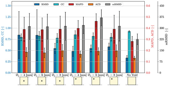
Figure 5.
Bar plot comparing the average and standard deviation of the obtained damage metrics, computed using the real component of the measured impedance from kHz to MHz (801 linearly spaced points).
Overall, one sees that all damage metrics increased significantly when damage was present, with the exception of the Correlation Coefficient, . This occurred because, as expected from its mathematical definition, the obtained metric values tended towards the unit value when the spectra being compared were similar in trend. Therefore, the , for the case where there was no void, had values between 0.90 and 0.95, while overall, the metric values from the damaged SLJs tended be be lower than 0.90.
This being said, there were some outlier values, originating from joints containing voids, that were superior to 0.90. These values tended to originate from the comparison between any given damaged joint specimen and the pristine SLJ 2 specimen, which was used as the reference baseline specimen for comparison. This can be explained by the fact that the spectra of the reference undamaged joint SLJ 2 were similar to some spectra from joints with voids. This was the case of specimen SLJ 1, which had a void in the corner of the overlap adhesive layer, and mm, as can be seen in Figure 6a, yielding . Conversely, Figure 6b shows a similar comparison of the spectra from the reference SLJ 1 with specimen SLJ 2, which had a mm void in the center of the overlap, obtaining a value of , which is to be expected.
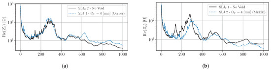
Figure 6.
Lin–Log plot comparing the Re() spectra between pristine SLJs and SLJs with voids. (a) Reference SLJ 2 and SLJ 1 (corner mm void) specimens. (b) Reference SLJ 1 and SLJ 2 (middle mm void) specimens.
As previously stated, the other four damage metrics—Root-Mean-Squared Deviation, , Mean Absolute Percentage Deviation, , modified Root-Mean-Squared Deviation, , and Averaged Canberra Distance, —increased with the presence of damage. This is to be expected, since bigger changes in the spectra translated into bigger distances between the sampled impedance values. Overall, the obtained metrics for damaged cases tended to have values between one- and two-times the metric values for undamaged joints, as shown in Figure 7. This is explained by the fact that the damage caused significant changes in the obtained spectra, as shown in Figure 6b. However, even with these four distance-based damage indices, there was some overlap between the undamaged and damaged adhesive joints, precisely in the case where undamaged SLJ 2 was used as a reference.
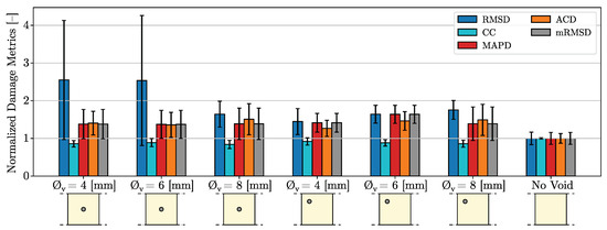
Figure 7.
Bar plot comparing the normalized average and standard deviation of the obtained damage metrics, computed using the real component of the measured impedance from kHz to MHz (801 linearly spaced points).
One must also note that the metric had a somewhat better performance in damage detection, when compared with the other three damage metrics. Normally, the metric values for the damaged SLJs tended to be between one- to two-times the observed values from the undamaged joints. However, some values were approximately five-times what was observed for undamaged joints, hence the large standard deviation bars observed in the cases of voids with a diameter mm, which were placed in the middle of the overlap. This can only be caused by the fact that the second uncontrolled source of damage (increasing the overall void area) occupied a bigger area of the overlap and, thus, caused a bigger change in the impedance spectrum. Furthermore, one must point out that the metric overall had a better performance in damage detection. This is noted by the fact that, in other cases of void size and placement, there was a smaller, but significant improvement in damage detection ((12.5, 12.5) mm, mm, or (6.25, 6.25) mm, mm damage cases), when compared to the other three distance-based damage indices.
4.1.2. Logarithmically Spaced Spectrum from kHz to MHz
Figure 8 plots the average and standard deviation of the damage indices that were computed with logarithmically spaced measured impedance, from kHz to MHz.
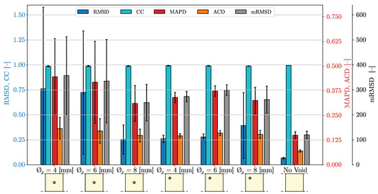
Figure 8.
Plot comparing the average and standard deviation of the obtained damage metrics, computed using the real component of the measured impedance from kHz to MHz (801 logarithmically spaced points).
In an initial analysis, one sees that the metric appeared to have very little changes between damage cases. Upon closer attention, one can verify that the metrics from the pristine SLJs were indeed very close to the average value of with very little variation (). Conversely, all of the computed for the damaged cases yielded values between 0.9792 and 0.9972, which means that some overlap still existed. Furthermore, all six classes of damaged joints had larger standard deviation. The smallest standard deviation for damaged adhesive joints was from the joints that had a void of diameter mm in the corner of the overlap, i.e., mm, where . In essence, the correlation coefficient was unreliable in the damage detection, when using this spectral measurement condition.
All distance-based damage metrics (, , , and ) had a clearer distinction between joints with and without artificially created voids. Indeed, the average values for all six damage cases tended to be two- to three-times higher than the average value observed for the pristine case. This is shown in Figure 9, with a zoomed view of the , , and for one case (void in mm, with mm) as an example. Overall, for these three mathematical metrics, all values from the damaged joints tended to have values between 1.5- and 4-times the values observed for the undamaged adhesive joint specimens.
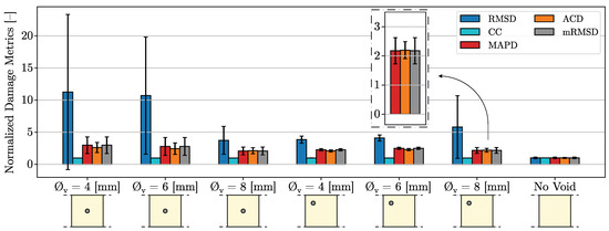
Figure 9.
Bar plot comparing the normalized average and standard deviation of the obtained damage metrics, computed using the real component of the impedance from kHz to MHz (801 logarithmically spaced points).
A similar behavior was observed for the index values. However, the gap in values between measurements of the damaged and pristine SLJs was starker, since, as shown for the previous case, this damage metric appeared to have a better performance in damage detection. This can be seen by the fact that all average values for damaged instances were at least four-times higher than the average for the undamaged case. In part, this can be explained by the mathematical definition of the damage index, which enables a better detection of damage, as previously stated. However, one must point out that all four distance-based damage metrics were computed from measurements with 801 logarithmically spaced sampling points, which means that each order of magnitude of the frequency had 267 sampled impedance points. This equal distribution of the sampled points enabled the lower frequency range (i.e., below 100 kHz) of the measured real component of impedance, Re(), to have a bigger impact on damage detection.
It is noted that the average and standard deviation of the , , and values, for the two cases where voids of mm, placed in the middle of the overlap (i.e, void in mm), were higher than for the remaining damaged joint classes. This was caused by the fact that some SLJs in these classes had a larger overall damaged area due to the unwanted creation of a second defect in the adhesive layer. However, with the use of logarithmically spaced impedance spectra, the differences occurring at lower frequencies were more pronounced, and the and metrics also became more sensitive to the impedance alterations.
4.1.3. Linearly Spaced Spectrum from kHz to MHz
Figure 10 shows the average and standard deviation of the computed damage indices from the linearly spaced measured impedance, from kHz to MHz.
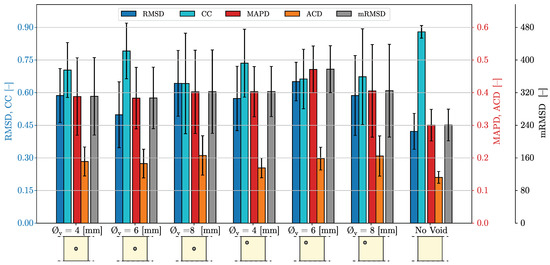
Figure 10.
Plot comparing the average and standard deviation of the obtained damage metrics, computed using the real component of the measured impedance from kHz to MHz (801 linearly spaced points).
Much like in the previous cases, the metric decreased with an increasing change in the spectra of Re(), according to its mathematical definition. Furthermore, the global average of all metrics clearly showed the presence of damage, since the average value for the undamaged joints was , while all of the average values for the damaged SLJs were below 0.80, . Despite this, some outlier values existed, much in the same line as seen in the metrics of the linearly spaced sampled frequencies from kHz to MHz, meaning that some of the computed metric values for the damaged joints fell within the value range of the undamaged SLJ specimens. This overlap can be visualized in the bar plot of Figure 11, which shows the normalized metrics according to the average value of the no void case.
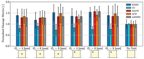
Figure 11.
Bar plot comparing the normalized average and standard deviation of the obtained damage metrics, computed using the real component of the measured impedance from kHz to MHz (801 linearly spaced points).
Furthermore, similar to the metric results from the 801 linearly spaced sampled frequencies from kHz to MHz, there was an overlap in the metric values between the undamaged and damaged cases when using the , , , and distance-based metrics. Likewise, this can be seen in the normalized damage metric bar plot of Figure 11, where there is an overlap of the various standard deviation bars between most cases of the joints with voids and the case of the undamaged joints. These similarities in trends between both spectral cases were due to the fact that a significant portion of the linearly sampled measured impedance spectra between kHz and MHz was equivalent to the direct spectral measurements from kHz to MHz. Therefore, the obtained metrics should be similar to the ones obtained in the first analyzed spectral case, as was the case when comparing Figure 5 and Figure 10. The only difference between both cases that impacted the computed metrics was the fact that this spectral condition did not have the initial exponential decrease of Re(), thus leading to a slight decrease of the metric values when compared to the first studied case.
Upon closer comparison between the Averaged Canberra Distance, , and the other three distance-based metrics, one sees that there were fewer cases of damaged joints with overlapping values with the undamaged adhesive joints. This can be attributed to one of the base properties of the Canberra distance as a mathematical index, which is the fact that it is sensitive to alterations near zero [40,41]. Consequently, the is a somewhat more-robust damage index when compared to the , , and .
4.1.4. Logarithmically Spaced Spectrum from kHz to kHz
Figure 12 shows the average and standard deviation of the computed damage indices from the logarithmically spaced measured impedance, from kHz to kHz. Note that this impedance spectrum was obtained by cropping the measured logarithmically spaced impedance spectrum from kHz to MHz, obtaining a sub-spectrum with 347 sampled points.

Figure 12.
Plot comparing the average and standard deviation of the obtained damage metrics, computed using the real component of the measured impedance from kHz to kHz (347 logarithmically spaced points).
An initial observation showed that, once again, as per the mathematical definition, a comparison of the undamaged joints with a reference joint yielded higher values, when compared to the metrics obtained for the damaged joints as a whole. In this manner, the mean value for the pristine SLJs was of , while the average values for all three damaged cases tended to be below 0.865. However, upon closer observation, a significant portion of the computed correlation coefficient values for the damaged bonded joints, using the SLJ 2 specimen as a reference, overlapped significantly with the values obtained for the undamaged joints. Comparatively speaking, there was no overlap between the damaged and undamaged joints when using SLJ 1 as a reference, and three values of the damaged joints overlapped with the undamaged values when SLJ 3 was used as a reference. Alternatively, Figure 13, which presents the normalized average damage metrics for this spectral condition, shows that there was a clear overlap between the undamaged and damaged metrics, which corroborated the obtained results.
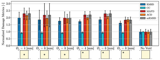
Figure 13.
Bar plot comparing the normalized average and standard deviation of the obtained damage metrics, computed using the real component of the measured impedance from kHz to kHz (347 logarithmically spaced points).
Converse to the statistical damage metric, there was no overlap between the damaged and undamaged joints when using all four distance-based metrics—, , , and . While inspecting these four metrics, one sees that both the average and values for all six different void positions tended to be at least double those of the undamaged SLJs.
Furthermore, while the overall differentiation between the damaged and undamaged cases was less noticeable when using the Averaged Canberra Distance, , one sees that, when examining all individual values, there was a bigger gap between the maximum value from an undamaged joint and the minimum value form a damaged joint. In this manner, all metrics from the damaged joints were closer together, and consequently, the standard deviations for each void placement were smaller, as seen in Figure 12 and Figure 13. This was further proof that the damage index is sensitive to alterations near zero [40,41], thus proving itself as a reliable metric for better damage detection. While a similar thing can be said for the results of the for this spectral case, one sees that, in relative terms, the gap between the maximum value from an undamaged joint and the minimum value form a damaged joint was comparatively smaller than the respective gap of the metric.
4.1.5. Combination of the Three Measured Spectra from kHz to MHz
Figure 14 shows the average and standard deviation of the damage metrics computed by joining the three originally measured impedance spectra, thus obtaining a resultant spectrum of a frequency range of kHz, with a total of 2389 sampled points. With this case, one hopes that more sampled points will enable a better understanding of the integrity of the SLJ specimens.
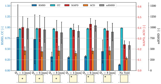
Figure 14.
Plot comparing the average and standard deviation of the obtained damage metrics, computed using the real component of the measured impedance from kHz to MHz (2389 spaced points).
As with the previous impedance spectral case, a quick overview of the showed that the impedance spectra from the undamaged joints were similar, thus having index values closer to the unit value, when compared to the values from the damaged joints. However, when comparing to both the values obtained for the directly measured linearly and logarithmically sampled spectra, these results were much closer to the ones obtained in the logarithmically sampled spectra. This can be stated since the average values calculated from the linearly spaced spectra (frequency range kHz with 801 sampled frequencies) had a wider dispersion, , while for the logarithmically spaced spectra (frequency range kHz with 801 sampled frequencies), a smaller dispersion was observed, . For comparison, this combination of the three spectra yielded average values varying between 0.967 and 0.988.
Unsurprisingly and in the same fashion as in previous spectral case studies, there was a considerable overlap between the metric values from the undamaged and damaged cases, which were mostly present when using the impedance spectra of the reference specimen SLJ 2, which can be attributed to the lack of significant spectral differences, as shown in Figure 6a.
Regarding the four distance-based metrics, , , , and , one sees that there was a clearer distinction between the damaged and undamaged cases. When analyzing the results obtained for the , , and damage metrics, one sees that all metric averages for all six damaged cases were 1.5- to 2-times higher than the average values for undamaged joints, as shown in Figure 15. However, upon closer examination, one sees that there was a slight overlap in the values between the undamaged and damaged joints when using the and metrics. For instance, the computed index for the SLJ 2 specimen with a void in the middle of the adhesive layer ( mm) was 0.2591 when the maximum value obtained for an undamaged joint was of 0.2604. Likewise, for the same artificially damaged joint, a value of 619 was obtained, when the maximum metric value from an undamaged joint was 622. This small overlap (or near overlap) does not occur with the index, which yielded average values 2-times or higher for the damaged cases, when compared with the baseline undamaged case. This is also illustrated in Figure 15.

Figure 15.
Bar plot comparing the normalized average and standard deviation of the obtained damage metrics, computed using the real component of the measured impedance from kHz to MHz (2389 spaced points).
When comparing this spectral case with both the originally measured linearly and logarithmically spaced spectra results, one sees that the , , and attained similar values to the ones obtained with the metrics from the linearly sampled frequency spectra. However, the metric can take advantage of the added spectral information by combining all three directly measured spectra, thus obtaining values that range between the ones yielded in the linearly sampled spectra and the ones from the logarithmically spaced spectra.
4.2. Metrics Using the Complex Active Impedance
4.2.1. Linearly Spaced Spectrum from kHz to MHz
Figure 16a,b present the average and standard deviation of the proposed , , and metrics, which were compared to their equivalent metrics that use exclusively the real component, Re(). Note that, in Figure 16a, two different metrics are presented, one using the measured impedance, , and a second one using the active impedance, , as specified in Equation (3b).
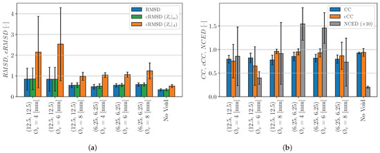
Figure 16.
Bar plot comparing the proposed complex damage metrics with their original ones from the impedance spectra from kHz to MHz (801 spaced points). (a) Comparison between the and (with both measured and active impedances, and , respectively). (b) Comparison between the and (with active impedance, ).
From Figure 16a, one sees that there was virtually no difference between the traditional metric and the that was computed using the measured impedance. This was the case since the imaginary component of the impedance was mainly composed by the passive impedance, as described in Equation (3a) [14]. Therefore, performing the difference operation between the imaginary components of the reference impedance, Im(), and of the electrical impedance of the joint being inspected, Im(), will yield an almost null result, resulting in similar values to the ones obtained with the index.
Conversely, removing the passive component of the impedance, as per Equation (3a), should yield better results, as shown in Figure 16a, where the average values for all six damaged cases, and for the pristine case, are twice those of the values obtained for the index. In this manner, despite the fact that there was a wide dispersion of values for the damaged cases, there was a wide gap when compared to the values obtained for the undamaged SLJs.
The metric, which can be viewed as loosely inspired by the proposed metric, presented a completely different behavior, as shown in Figure 16b. Note that the obtained values were one order of magnitude smaller than as actually represented here. As with most metrics presented so far, the metric values obtained for the no void case were concentrated, having an average value of and a small standard deviation of . Conversely, the damaged adhesive joints tended to have higher damage metric values. Note that a couple of outlier values existed with this metric or, in other words, some values from the damaged joints were in the same range of values as the values from the undamaged joints.
However, unlike with other damage metrics, one sees that the maximum damage metric values did not occur in the SLJs with voids of diameter mm in the middle of the overlap, but occurred in the SLJs with voids of diameter mm in the corner of the overlap. The only other metrics that followed a similar pattern were the and metrics, but to a lesser degree.
Furthermore, from Figure 16b, one sees a comparison between the obtained values, which were calculated with the real component of the measured electrical impedance, Re(), and the complex Correlation Coefficient values, , which made use of both the real and imaginary components of the active impedance, Re() and Im(), respectively. While the metric was able to differentiate between damaged and undamaged adhesive joints, the index was unable to achieve this, since there was a large overlap of between the damaged and undamaged specimens. One must point out that the only reason why the average values were lower for the damage classes, mm, mm, was that some extremely lower values existed for these cases. In this manner, while can indeed help in the task of damage detection, this was not the trend observed for this case.
Figure 17 plots the measured and active electrical impedances, and , respectively. One sees that the active impedance was significantly different in three regards. Firstly, the imaginary component had a significant change in behavior, having positive values throughout the frequency range in the analysis. Consequently, one can say that the capacitive behavior present in the passive component of the measured impedance was removed and that the resultant active impedance had an inductive behavior.
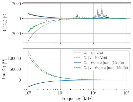
Figure 17.
Plot comparing the measured and active impedances, and , respectively, from an undamaged and a damaged adhesive joint specimen, for the frequency range of kHz.
Secondly, the peaks observed in the real component of the active impedance, Re(), had increased amplitudes. This was because, while removing the passive impedance, as described in Equation (3a), the added influence of the dielectric loss factor, , was also removed. In this manner, a passive resistive component was also removed from the measured impedance, enabling better damage detection.
However, thirdly, and more importantly, in the beginning of the frequency range in the analysis, one sees that negative resistive values were observed in the active impedance. At first glance, this result seems physically impossible, since negative resistance values are physically impossible to obtain, unless special electronic circuits are employed that receive energy from outside the electrical system in question [43]. However, the piezoceramic material used in this piezoelectric element was a modified lead zirconate titanate material, thus meaning that the added chemical elements into the ceramic may significantly influence the material properties. Although the authors do not know the chemical composition of the PIC 255 piezoceramic material, research has shown that modified lead zirconate titanate materials may have dielectric constant values varying with the excitation frequency [44].
Given this, the dielectric constant value given by the sensor manufacturer may only be applicable in a portion of the frequency range in question. As such, when considering the active impedance for damage detection, this paper only tackled the linearly spaced active impedance spectra from kHz to MHz and the logarithmically spaced active impedance spectra from kHz to kHz, given that these ranges did not appear to have negative values of Re() or the influence of such values may be comparatively smaller in damage detection.
4.2.2. Linearly Spaced Spectrum from kHz to MHz
Figure 18a,b present the average and standard deviation of the proposed , , and metrics, which were compared to their equivalents that use exclusively the real component, Re(). Note that, in Figure 18a, the metric was computed using the active impedance, , as specified in Equation (3b), since, as previously shown, the imaginary component of the measured impedance did not contribute to the damage detection.
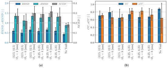
Figure 18.
Bar plot comparing the proposed complex damage metrics with their original ones from the impedance spectra from kHz to MHz (801 spaced points). (a) Comparison between the , , and . (b) Comparison between the and .
From the analysis of Figure 18a, one sees that the index, which was computed using the active impedance, , yielded higher values overall, when compared with the , which was computed with only the real component of the measured impedance, Re(). Furthermore, when compared with the damage index, there was considerably less overlap of the damage metric values between the results of the classes of the SLJs with a void and the undamaged adhesive joints when using the . This can be seen by the fact that there was a significant overlap of the standard distribution between the damaged and undamaged cases, when viewing the metric, while, conversely, this overlap only occurred between the no void and mm, mm, cases, when viewing the metric results. Furthermore, this overlap reduction was achieved despite the fact that the average values of and for the damaged cases tended to be approximately 1.5-times those of the average value for the no void case.
This increased accuracy of the occurred in a spectral region where significant overlap occurred, as seen in the previous subsection. However, a comparison between the measured impedance, , and the active impedance, , as presented in Figure 19 revealed that the removal of the passive component of the impedance yielded a spectral region that appeared more sensitive to the mechanical integrity of the adhesive joint. This was the case both for the real and imaginary components, Re() and Im(), respectively, and was especially pronounced at the beginning of the frequency range under study (below 300 kHz).
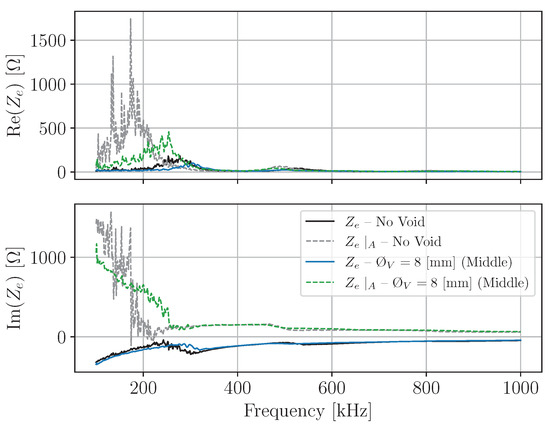
Figure 19.
Plot comparing the measured and active impedances, and , respectively, from an undamaged and a damaged adhesive joint specimen, for the frequency range of kHz.
However, this increased performance was only observed for the and was not verified for the proposed metric, which had a significant overlap in metric values between the damaged and undamaged cases. Indeed, a comparison between the average values of the and metrics showed that there was a smaller gap (in absolute and relative terms) between the average value of the no void case and the average for the same metric for the mm, mm case, when compared to the metric.
This difference in performance can be attributed to two distinct causes. Firstly, most cases of the damage metric values of the damaged joints overlapping with the values from the no void case corresponded to the cases where the reference undamaged joint was SLJ 2. In this manner, the issue first pointed out with the help of Figure 6 persisted if proper damage metrics were not chosen. However, it is also noted that the metric yielded comparatively smaller values overall, thus making the damage detection comparatively harder than with the metric.
Finally, with the analysis of Figure 18b, one sees that the complex Correlation Coefficient, , had a terrible performance in the damage detection, even when compared with the traditional metric or when compared with the results obtained in the previous spectral case study. Indeed, it appeared that the imaginary component, Im(), may have significant changes in values between the damaged and undamaged cases, as shown in Figure 19, and no clear trend can be seen with this specific metric since the active impedance can have significant changes.
4.2.3. Logarithmically Spaced Spectrum from kHz to kHz
Figure 20a,b display the average and standard deviation of the proposed , , and metrics, which were compared to their equivalents that use exclusively the real component, Re(). Note that this impedance spectrum was obtained by cropping the measured logarithmically spaced impedance spectrum from kHz to MHz, obtaining a sub-spectrum with 347 sampled points.
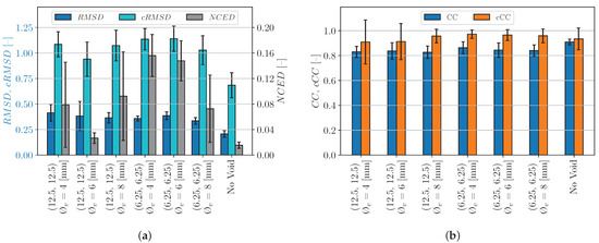
Figure 20.
Bar plot comparing the proposed complex damage metrics with their original ones from the impedance spectra from kHz to MHz (347 logarithmically spaced points). (a) Comparison between the , , and . (b) Comparison between the and .
From Figure 20a, one sees, once again, that the metric values, which were computed with both the real and imaginary components of the active impedance, Re() and Im(), respectively, were overall comparatively higher than what was obtained with the index, which was computed with only the real component of the measured impedance, Re(). However, unlike with the index, where no overlap of the metric values between the damaged and undamaged joints existed, in the case of the metric, some overlap existed. In this case, the outlier value may be present in the no void class, since the value comparing the spectra of the undamaged SLJ 3 with the reference SLJ 2 was approximately 0.9140, which was approximately equal to the sum between the average value for the specific class and twice the standard deviation or, in other words,
Therefore, and once again, the issue first pointed out with the help of Figure 6 may persist. However, despite this, overall, the metric was helpful in the damage detection, as seen by the fact that all average values for the six different cases of voids were twice that of the no void case.
Conversely, there was little overlap between the values of the for the undamaged and damaged joints. Furthermore, the overlap only occurred for the damaged case of voids in the mm, mm case. This was also the class of the adhesive joints with voids, with the lowest average value of the metric. However, for this case, the average value still was considerably higher than for undamaged joints. In this manner, this may indeed have occurred due to the fact that the active impedance spectra were less pronounced for the specimens of this specific case. However, to the best of the authors’ knowledge, there was no specific explanation for this, since, for instance, the metric was able to better detect damages in this class.
Finally, the complex Correlation Coefficient, , was once again unable to effectively differentiate between the damaged and undamaged adhesive joints. This may be due to the fact that the real component of the active impedance was more sensitive to the damage than the actual real component of the measured impedance, but no real change in the shape of the overall impedance spectra occurred, as seen in Figure 21.
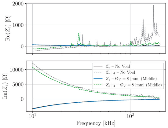
Figure 21.
Plot comparing the measured and active impedances, and , respectively, from an undamaged and a damaged adhesive joint specimen, for the frequency range of kHz.
5. Conclusions
This paper studied the feasibility of using EMIS-based damage metrics for void detection in adhesive SLJ specimens with the help of experimentally obtained electric impedance spectra. Four traditional damage metrics were tested in this research—the Root-Mean-Squared Deviation, , the Mean Absolute Percentage Deviation, , the Correlation Coefficient, , and the modified Root-Mean-Squared Deviation, —which make use of the real component of the measured electrical impedance. Likewise, a new metric was proposed that makes use of this component, which is the Averaged Canberra Distance, . Furthermore, three new damage metrics were also proposed that can use the real and imaginary components of the active impedance, which were more sensitive to damage. These were the complex Root-Mean-Squared Deviation index, , the Normalized Complex Euclidean Distance, , and the complex Correlation Coefficient, .
From this study, one can conclude that, overall, the Root-Mean-Squared Deviation, , was able to better differentiate between damaged and undamaged joints, especially when studying the whole frequency range in question, which was kHz. In this manner, the values from the damaged joints tended to be double the metric values from the undamaged joints, with some extreme values being over ten-times higher. Conversely, the Averaged Canberra Distance, , which is based on the Canberra Distance, could perform better in the damage detection when other metrics showed a large overlap between the damaged an undamaged cases. While the Correlation Coefficient, , could also help in a significant manner in the task of void detection, the obtained results were also strongly dependent on the spectral frequency conditions. The Mean Absolute Percentage Deviation, , and the modified Root-Mean-Squared Deviation, , permitted the damage detection, but were overall less exact in distinguishing between the damaged and pristine SLJs. The only exception to this occurred with the logarithmically sampled spectral measurement of kHz.
Damage metrics that make use of the active impedance were also able to detect the damage in the adhesive joints. The complex Root-Mean-Squared Deviation index, , allowed for better damage detection, when compared to the traditional index. Meanwhile, the Normalized Complex Euclidean Distance, , showed itself to be sensitive to the damage present in the corner of the overlap, while most other metrics were more sensitive to the damage in the middle of the overlap. Despite these interesting results, the complex Correlation Coefficient, , appeared to be the most-ill-suited metric for damage detection, since, despite the fact that the active impedance was more sensitive to the mechanical changes in the structure, these changes were more pronounced in the peaks, rather than the changes in the overall spectra.
Author Contributions
Conceptualization, A.F.G.T., A.M.L. and L.F.M.d.S.; investigation, A.F.G.T.; methodology A.F.G.T. and A.M.L.; formal analysis A.F.G.T.; resources, A.M.L. and L.F.M.d.S.; data curation A.F.G.T.; supervision, A.M.L. and L.F.M.d.S.; writing—original draft, A.F.G.T.; writing—review and editing, A.M.L. and L.F.M.d.S. All authors have read and agreed to the published version of the manuscript.
Funding
The authors gratefully acknowledge the funding of Grant 2021.07689.BD, which was provided by Fundação para a Ciência e Tecnologia (FCT).
Institutional Review Board Statement
Not applicable.
Informed Consent Statement
Not applicable.
Data Availability Statement
Not applicable.
Conflicts of Interest
The authors declare no conflict of interest.
Appendix A. Metrics
Appendix A.1. Metrics Using the Real Component of the Impedance
Appendix A.1.1. Linearly Spaced Spectrum from fi = 1 kHz to ff = 1 MHz
This subsection will present all of the obtained metrics for damage detection using the linearly spaced measured impedance spectrum from kHz to MHz.
Table A1.
damage metric results for linearly spaced impedance spectra (801 points), from kHz to MHz (damage location and diameter in mm).
Table A1.
damage metric results for linearly spaced impedance spectra (801 points), from kHz to MHz (damage location and diameter in mm).
| Case | (12.5, 12.5) | (12.5, 12.5) | (12.5, 12.5) | (6.25, 6.25) | (6.25, 6.25) | (6.25, 6.25) | No Void |
|---|---|---|---|---|---|---|---|
| Reference SLJ for Damage Metric Calculation: SLJ 1 | |||||||
| Mean | 0.881747 | 0.847592 | 0.620563 | 0.541951 | 0.615546 | 0.631591 | 0.314935 |
| 0.531134 | 0.612240 | 0.094997 | 0.144474 | 0.049026 | 0.049174 | 0.065269 | |
| SLJ 1 | 0.508978 | 1.554390 | 0.600701 | 0.377542 | 0.559442 | 0.583762 | nan |
| SLJ 2 | 1.489896 | 0.481300 | 0.723921 | 0.648654 | 0.650143 | 0.682007 | 0.361087 |
| SLJ 3 | 0.646365 | 0.507087 | 0.537067 | 0.599656 | 0.637053 | 0.629004 | 0.268783 |
| Reference SLJ for Damage Metric Calculation: SLJ 2 | |||||||
| Mean | 0.802185 | 0.847246 | 0.440877 | 0.408856 | 0.454990 | 0.516274 | 0.383830 |
| 0.707944 | 0.732888 | 0.091309 | 0.045811 | 0.017794 | 0.110137 | 0.040763 | |
| SLJ 1 | 0.336837 | 1.687976 | 0.470309 | 0.376610 | 0.463022 | 0.438675 | 0.412654 |
| SLJ 2 | 1.616902 | 0.510577 | 0.513840 | 0.461294 | 0.467351 | 0.467816 | nan |
| SLJ 3 | 0.452817 | 0.343185 | 0.338481 | 0.388664 | 0.434596 | 0.642331 | 0.355007 |
| Reference SLJ for Damage Metric Calculation: SLJ 3 | |||||||
| Mean | 0.858162 | 0.832527 | 0.576104 | 0.491676 | 0.566757 | 0.601925 | 0.297836 |
| 0.562824 | 0.633286 | 0.093154 | 0.127461 | 0.040423 | 0.046103 | 0.030430 | |
| SLJ 1 | 0.468224 | 1.563525 | 0.563547 | 0.347402 | 0.524166 | 0.548896 | 0.276318 |
| SLJ 2 | 1.503389 | 0.450235 | 0.674900 | 0.589012 | 0.604591 | 0.632492 | 0.319353 |
| SLJ 3 | 0.602873 | 0.483820 | 0.489866 | 0.538615 | 0.571515 | 0.624387 | nan |
| Overall Damage Metric Data | |||||||
| Mean | 0.847365 | 0.842455 | 0.545848 | 0.480828 | 0.545764 | 0.583263 | 0.332200 |
| 0.525611 | 0.572983 | 0.114362 | 0.114857 | 0.078549 | 0.082811 | 0.055022 | |
Table A2.
damage metric results for linearly spaced impedance spectra (801 points), from kHz to MHz (damage location and diameter in mm).
Table A2.
damage metric results for linearly spaced impedance spectra (801 points), from kHz to MHz (damage location and diameter in mm).
| Case | (12.5, 12.5) | (12.5, 12.5) | (12.5, 12.5) | (6.25, 6.25) | (6.25, 6.25) | (6.25, 6.25) | No Void |
|---|---|---|---|---|---|---|---|
| Reference SLJ for Damage Metric Calculation: SLJ 1 | |||||||
| Mean | 331.06 | 294.04 | 338.63 | 333.68 | 368.98 | 326.92 | 199.01 |
| 72.06 | 84.17 | 64.91 | 19.17 | 15.50 | 82.78 | 19.71 | |
| SLJ 1 | 259.67 | 377.44 | 376.68 | 325.68 | 361.15 | 378.91 | nan |
| SLJ 2 | 329.75 | 209.13 | 375.53 | 319.82 | 386.84 | 370.40 | 212.94 |
| SLJ 3 | 403.76 | 295.55 | 263.68 | 355.56 | 358.96 | 231.46 | 185.07 |
| Reference SLJ for Damage Metric Calculation: SLJ 2 | |||||||
| Mean | 229.78 | 264.24 | 227.36 | 256.24 | 315.38 | 242.75 | 260.31 |
| 46.75 | 60.57 | 83.93 | 38.30 | 32.69 | 73.54 | 32.15 | |
| SLJ 1 | 216.96 | 327.65 | 312.52 | 297.75 | 285.44 | 322.51 | 237.57 |
| SLJ 2 | 190.78 | 206.98 | 224.85 | 248.71 | 350.26 | 228.13 | nan |
| SLJ 3 | 281.61 | 258.10 | 144.71 | 222.27 | 310.44 | 177.62 | 283.05 |
| Reference SLJ for Damage Metric Calculation: SLJ 3 | |||||||
| Mean | 373.34 | 370.78 | 372.65 | 367.46 | 425.29 | 370.32 | 217.46 |
| 84.22 | 93.09 | 82.76 | 31.05 | 37.04 | 124.60 | 34.30 | |
| SLJ 1 | 306.20 | 461.75 | 438.30 | 384.21 | 396.95 | 473.29 | 193.20 |
| SLJ 2 | 345.97 | 275.71 | 399.97 | 331.63 | 467.20 | 405.84 | 241.72 |
| SLJ 3 | 467.84 | 374.88 | 279.69 | 386.55 | 411.72 | 231.82 | nan |
| Overall Damage Metric Data | |||||||
| Mean | 311.39 | 309.69 | 312.88 | 319.13 | 369.88 | 313.33 | 225.59 |
| 87.75 | 84.38 | 94.12 | 56.02 | 54.18 | 100.51 | 36.21 | |
Table A3.
damage metric results for linearly spaced impedance spectra (801 points), from kHz to MHz (damage location and diameter in mm).
Table A3.
damage metric results for linearly spaced impedance spectra (801 points), from kHz to MHz (damage location and diameter in mm).
| Case | (12.5, 12.5) | (12.5, 12.5) | (12.5, 12.5) | (6.25, 6.25) | (6.25, 6.25) | (6.25, 6.25) | No Void |
|---|---|---|---|---|---|---|---|
| Reference SLJ for Damage Metric Calculation: SLJ 1 | |||||||
| Mean | 0.413307 | 0.367095 | 0.422759 | 0.416585 | 0.460652 | 0.408145 | 0.248447 |
| 0.089958 | 0.105075 | 0.081034 | 0.023931 | 0.019352 | 0.103350 | 0.024605 | |
| SLJ 1 | 0.324176 | 0.471213 | 0.470262 | 0.406586 | 0.450877 | 0.473046 | nan |
| SLJ 2 | 0.411675 | 0.261088 | 0.468822 | 0.399275 | 0.482942 | 0.462423 | 0.265845 |
| SLJ 3 | 0.504069 | 0.368982 | 0.329192 | 0.443894 | 0.448138 | 0.288964 | 0.231049 |
| Reference SLJ for Damage Metric Calculation: SLJ 2 | |||||||
| Mean | 0.286868 | 0.329890 | 0.283845 | 0.319902 | 0.393731 | 0.303061 | 0.324982 |
| 0.058370 | 0.075621 | 0.104784 | 0.047818 | 0.040814 | 0.091812 | 0.040142 | |
| SLJ 1 | 0.270860 | 0.409055 | 0.390161 | 0.371724 | 0.356351 | 0.402630 | 0.296597 |
| SLJ 2 | 0.238173 | 0.258398 | 0.280711 | 0.310496 | 0.437277 | 0.284804 | nan |
| SLJ 3 | 0.351572 | 0.322219 | 0.180664 | 0.277486 | 0.387564 | 0.221749 | 0.353366 |
| Reference SLJ for Damage Metric Calculation: SLJ 3 | |||||||
| Mean | 0.466087 | 0.462891 | 0.465237 | 0.458756 | 0.530950 | 0.462320 | 0.271486 |
| 0.105149 | 0.116214 | 0.103318 | 0.038766 | 0.046239 | 0.155551 | 0.042828 | |
| SLJ 1 | 0.382272 | 0.576461 | 0.547197 | 0.479664 | 0.495571 | 0.590879 | 0.241202 |
| SLJ 2 | 0.431917 | 0.344202 | 0.499334 | 0.414025 | 0.583270 | 0.506670 | 0.301769 |
| SLJ 3 | 0.584071 | 0.468010 | 0.349180 | 0.482579 | 0.514010 | 0.289410 | nan |
| Overall Damage Metric Data | |||||||
| Mean | 0.388754 | 0.386625 | 0.390614 | 0.398414 | 0.461778 | 0.391175 | 0.281638 |
| 0.109546 | 0.105345 | 0.117498 | 0.069938 | 0.067644 | 0.125476 | 0.045206 | |
Table A4.
damage metric results for linearly spaced impedance spectra (801 points), from kHz to MHz (damage location and diameter in mm).
Table A4.
damage metric results for linearly spaced impedance spectra (801 points), from kHz to MHz (damage location and diameter in mm).
| Case | (12.5, 12.5) | (12.5, 12.5) | (12.5, 12.5) | (6.25, 6.25) | (6.25, 6.25) | (6.25, 6.25) | No Void |
|---|---|---|---|---|---|---|---|
| Reference SLJ for Damage Metric Calculation: SLJ 1 | |||||||
| Mean | 0.739077 | 0.784894 | 0.712721 | 0.796544 | 0.752017 | 0.742571 | 0.927577 |
| 0.063712 | 0.120879 | 0.102763 | 0.106013 | 0.060672 | 0.097335 | 0.028361 | |
| SLJ 1 | 0.811437 | 0.652629 | 0.752830 | 0.918415 | 0.821075 | 0.737922 | nan |
| SLJ 2 | 0.691395 | 0.889643 | 0.595952 | 0.725643 | 0.707276 | 0.647644 | 0.907522 |
| SLJ 3 | 0.714400 | 0.812409 | 0.789381 | 0.745573 | 0.727700 | 0.842146 | 0.947631 |
| Reference SLJ for Damage Metric Calculation: SLJ 2 | |||||||
| Mean | 0.873875 | 0.872934 | 0.868886 | 0.924405 | 0.903613 | 0.871404 | 0.917079 |
| 0.057451 | 0.087767 | 0.053948 | 0.032939 | 0.028585 | 0.033853 | 0.013515 | |
| SLJ 1 | 0.923146 | 0.772023 | 0.872726 | 0.961476 | 0.931589 | 0.856564 | 0.907522 |
| SLJ 2 | 0.810770 | 0.931495 | 0.813121 | 0.898500 | 0.874456 | 0.847505 | nan |
| SLJ 3 | 0.887708 | 0.915284 | 0.920811 | 0.913240 | 0.904795 | 0.910143 | 0.926635 |
| Reference SLJ for Damage Metric Calculation: SLJ 3 | |||||||
| Mean | 0.775366 | 0.813026 | 0.755923 | 0.838629 | 0.796687 | 0.777016 | 0.937133 |
| 0.059034 | 0.112013 | 0.090588 | 0.086733 | 0.051527 | 0.080468 | 0.014847 | |
| SLJ 1 | 0.841546 | 0.694385 | 0.787170 | 0.938277 | 0.852763 | 0.768172 | 0.947631 |
| SLJ 2 | 0.728127 | 0.916958 | 0.653848 | 0.780127 | 0.751425 | 0.701336 | 0.926635 |
| SLJ 3 | 0.756424 | 0.827736 | 0.826751 | 0.797484 | 0.785874 | 0.861541 | nan |
| Overall Damage Metric Data | |||||||
| Mean | 0.796106 | 0.823618 | 0.779177 | 0.853193 | 0.817439 | 0.796997 | 0.927263 |
| 0.079750 | 0.101153 | 0.101469 | 0.090257 | 0.079621 | 0.087238 | 0.017944 | |
Table A5.
damage metric results for linearly spaced impedance spectra (801 points), from kHz to MHz (damage location and diameter in mm).
Table A5.
damage metric results for linearly spaced impedance spectra (801 points), from kHz to MHz (damage location and diameter in mm).
| Case | (12.5, 12.5) | (12.5, 12.5) | (12.5, 12.5) | (6.25, 6.25) | (6.25, 6.25) | (6.25, 6.25) | No Void |
|---|---|---|---|---|---|---|---|
| Reference SLJ for Damage Metric Calculation: SLJ 1 | |||||||
| Mean | 0.199087 | 0.176478 | 0.216578 | 0.172232 | 0.193134 | 0.207812 | 0.121839 |
| 0.024083 | 0.043029 | 0.037334 | 0.017802 | 0.024094 | 0.047329 | 0.011662 | |
| SLJ 1 | 0.171598 | 0.213994 | 0.218008 | 0.158128 | 0.176144 | 0.217648 | nan |
| SLJ 2 | 0.209190 | 0.129508 | 0.253176 | 0.166333 | 0.220708 | 0.249450 | 0.130085 |
| SLJ 3 | 0.216473 | 0.185931 | 0.178549 | 0.192234 | 0.182549 | 0.156338 | 0.113593 |
| Reference SLJ for Damage Metric Calculation: SLJ 2 | |||||||
| Mean | 0.138748 | 0.149336 | 0.144150 | 0.135678 | 0.167471 | 0.153320 | 0.140878 |
| 0.019474 | 0.030223 | 0.040807 | 0.012950 | 0.024146 | 0.035980 | 0.015264 | |
| SLJ 1 | 0.134801 | 0.175769 | 0.170352 | 0.148633 | 0.146410 | 0.183983 | 0.130085 |
| SLJ 2 | 0.121550 | 0.116387 | 0.164966 | 0.135666 | 0.193824 | 0.162266 | nan |
| SLJ 3 | 0.159894 | 0.155854 | 0.097133 | 0.122734 | 0.162178 | 0.113711 | 0.151672 |
| Reference SLJ for Damage Metric Calculation: SLJ 3 | |||||||
| Mean | 0.217853 | 0.211173 | 0.235850 | 0.192907 | 0.217909 | 0.228564 | 0.132632 |
| 0.027058 | 0.045375 | 0.041883 | 0.012986 | 0.034048 | 0.061819 | 0.026926 | |
| SLJ 1 | 0.192805 | 0.249831 | 0.247225 | 0.193571 | 0.189610 | 0.257388 | 0.113593 |
| SLJ 2 | 0.214203 | 0.161217 | 0.270870 | 0.179602 | 0.255694 | 0.270707 | 0.151672 |
| SLJ 3 | 0.246550 | 0.222470 | 0.189454 | 0.205548 | 0.208424 | 0.157596 | nan |
| Overall Damage Metric Data | |||||||
| Mean | 0.185229 | 0.178996 | 0.198859 | 0.166939 | 0.192838 | 0.196565 | 0.131783 |
| 0.041281 | 0.043891 | 0.054374 | 0.028163 | 0.032523 | 0.054514 | 0.017080 | |
Appendix A.1.2. Logarithmically Spaced Spectrum from fi = 1 kHz to ff = 1 MHz
This subsection will present all of the obtained metrics for damage detection using the logarithmically spaced measured impedance spectrum from kHz to MHz.
Table A6.
damage metric results for logarithmically spaced impedance spectra (801 points), from kHz to MHz (damage location and diameter in mm).
Table A6.
damage metric results for logarithmically spaced impedance spectra (801 points), from kHz to MHz (damage location and diameter in mm).
| Case | (12.5, 12.5) | (12.5, 12.5) | (12.5, 12.5) | (6.25, 6.25) | (6.25, 6.25) | (6.25, 6.25) | No Void |
|---|---|---|---|---|---|---|---|
| Reference SLJ for Damage Metric Calculation: SLJ 1 | |||||||
| Mean | 0.754661 | 0.716674 | 0.257899 | 0.258360 | 0.276146 | 0.394470 | 0.067530 |
| 0.930806 | 0.701788 | 0.157617 | 0.037594 | 0.033325 | 0.368588 | 0.012561 | |
| SLJ 1 | 0.202885 | 1.495496 | 0.438806 | 0.298382 | 0.305568 | 0.215461 | nan |
| SLJ 2 | 1.829335 | 0.521131 | 0.150194 | 0.252911 | 0.239956 | 0.149573 | 0.076413 |
| SLJ 3 | 0.231763 | 0.133395 | 0.184695 | 0.223788 | 0.282913 | 0.818376 | 0.058648 |
| Reference SLJ for Damage Metric Calculation: SLJ 2 | |||||||
| Mean | 0.773826 | 0.737301 | 0.247847 | 0.266245 | 0.282722 | 0.394143 | 0.072821 |
| 0.963189 | 0.730361 | 0.185275 | 0.049889 | 0.040746 | 0.399604 | 0.007618 | |
| SLJ 1 | 0.205004 | 1.543603 | 0.457289 | 0.320886 | 0.320673 | 0.216495 | 0.078208 |
| SLJ 2 | 1.885924 | 0.548240 | 0.105344 | 0.254724 | 0.239663 | 0.114166 | nan |
| SLJ 3 | 0.230551 | 0.120058 | 0.180909 | 0.223125 | 0.287831 | 0.851768 | 0.067434 |
| Reference SLJ for Damage Metric Calculation: SLJ 3 | |||||||
| Mean | 0.755157 | 0.717311 | 0.253401 | 0.256808 | 0.274928 | 0.391449 | 0.062505 |
| 0.935426 | 0.705344 | 0.162628 | 0.040437 | 0.034716 | 0.373832 | 0.005138 | |
| SLJ 1 | 0.200788 | 1.499863 | 0.439603 | 0.300294 | 0.306591 | 0.213582 | 0.058872 |
| SLJ 2 | 1.835167 | 0.521535 | 0.139217 | 0.249793 | 0.237806 | 0.139761 | 0.066138 |
| SLJ 3 | 0.229516 | 0.130536 | 0.181383 | 0.220338 | 0.280389 | 0.821004 | nan |
| Overall Damage Metric Data | |||||||
| Mean | 0.761215 | 0.723762 | 0.253049 | 0.260471 | 0.277932 | 0.393354 | 0.067619 |
| 0.816933 | 0.617223 | 0.146368 | 0.037464 | 0.031736 | 0.329886 | 0.008351 | |
Table A7.
damage metric results for logarithmically spaced impedance spectra (801 points), from kHz to MHz (damage location and diameter in mm).
Table A7.
damage metric results for logarithmically spaced impedance spectra (801 points), from kHz to MHz (damage location and diameter in mm).
| Case | (12.5, 12.5) | (12.5, 12.5) | (12.5, 12.5) | (6.25, 6.25) | (6.25, 6.25) | (6.25, 6.25) | No Void |
|---|---|---|---|---|---|---|---|
| Reference SLJ for Damage Metric Calculation: SLJ 1 | |||||||
| Mean | 356.74 | 323.07 | 250.73 | 272.21 | 295.22 | 257.15 | 110.72 |
| 179.92 | 191.42 | 71.76 | 15.92 | 8.76 | 51.92 | 14.63 | |
| SLJ 1 | 209.76 | 543.52 | 333.59 | 258.01 | 287.16 | 248.74 | nan |
| SLJ 2 | 557.38 | 226.87 | 210.32 | 269.20 | 293.95 | 209.95 | 121.06 |
| SLJ 3 | 303.07 | 198.83 | 208.28 | 289.42 | 304.55 | 312.77 | 100.37 |
| Reference SLJ for Damage Metric Calculation: SLJ 2 | |||||||
| Mean | 333.86 | 325.49 | 225.35 | 254.34 | 279.72 | 244.65 | 136.25 |
| 176.06 | 187.82 | 87.49 | 8.27 | 9.82 | 73.08 | 0.63 | |
| SLJ 1 | 201.23 | 539.08 | 325.88 | 259.78 | 270.55 | 247.22 | 136.70 |
| SLJ 2 | 533.61 | 251.27 | 166.47 | 244.82 | 278.52 | 170.31 | nan |
| SLJ 3 | 266.73 | 186.12 | 183.70 | 258.41 | 290.08 | 316.41 | 135.81 |
| Reference SLJ for Damage Metric Calculation: SLJ 3 | |||||||
| Mean | 381.32 | 357.19 | 271.33 | 294.04 | 323.58 | 281.32 | 112.61 |
| 177.90 | 196.11 | 83.49 | 16.46 | 12.91 | 50.65 | 8.67 | |
| SLJ 1 | 233.52 | 582.96 | 367.71 | 284.75 | 309.38 | 290.12 | 106.48 |
| SLJ 2 | 578.77 | 259.55 | 221.24 | 284.34 | 326.76 | 226.85 | 118.74 |
| SLJ 3 | 331.68 | 229.07 | 225.04 | 313.05 | 334.61 | 327.00 | nan |
| Overall Damage Metric Data | |||||||
| Mean | 357.31 | 335.25 | 249.13 | 273.53 | 299.51 | 261.04 | 119.86 |
| 155.49 | 166.93 | 73.09 | 21.09 | 21.36 | 53.96 | 14.83 | |
Table A8.
damage metric results for logarithmically spaced impedance spectra (801 points), from kHz to MHz (damage location and diameter in mm).
Table A8.
damage metric results for logarithmically spaced impedance spectra (801 points), from kHz to MHz (damage location and diameter in mm).
| Case | (12.5, 12.5) | (12.5, 12.5) | (12.5, 12.5) | (6.25, 6.25) | (6.25, 6.25) | (6.25, 6.25) | No Void |
|---|---|---|---|---|---|---|---|
| Reference SLJ for Damage Metric Calculation: SLJ 1 | |||||||
| Mean | 0.445365 | 0.403336 | 0.313020 | 0.339841 | 0.368563 | 0.321040 | 0.138221 |
| 0.224614 | 0.238981 | 0.089593 | 0.019874 | 0.010937 | 0.064820 | 0.018269 | |
| SLJ 1 | 0.261874 | 0.678546 | 0.416463 | 0.322116 | 0.358505 | 0.310532 | nan |
| SLJ 2 | 0.695855 | 0.283236 | 0.262572 | 0.336081 | 0.366977 | 0.262116 | 0.151140 |
| SLJ 3 | 0.378366 | 0.248226 | 0.260025 | 0.361326 | 0.380207 | 0.390472 | 0.125303 |
| Reference SLJ for Damage Metric Calculation: SLJ 2 | |||||||
| Mean | 0.416799 | 0.406353 | 0.281331 | 0.317527 | 0.349210 | 0.305425 | 0.170106 |
| 0.219804 | 0.234480 | 0.109221 | 0.010325 | 0.012262 | 0.091240 | 0.000783 | |
| SLJ 1 | 0.251219 | 0.673004 | 0.406836 | 0.324324 | 0.337765 | 0.308636 | 0.170660 |
| SLJ 2 | 0.666176 | 0.313694 | 0.207824 | 0.305646 | 0.347712 | 0.212622 | nan |
| SLJ 3 | 0.333001 | 0.232360 | 0.229333 | 0.322610 | 0.362152 | 0.395017 | 0.169552 |
| Reference SLJ for Damage Metric Calculation: SLJ 3 | |||||||
| Mean | 0.476059 | 0.445932 | 0.338736 | 0.367097 | 0.403972 | 0.351214 | 0.140584 |
| 0.222097 | 0.244835 | 0.104232 | 0.020550 | 0.016115 | 0.063235 | 0.010821 | |
| SLJ 1 | 0.291533 | 0.727788 | 0.459062 | 0.355491 | 0.386245 | 0.362203 | 0.132932 |
| SLJ 2 | 0.722560 | 0.324029 | 0.276203 | 0.354975 | 0.407935 | 0.283205 | 0.148235 |
| SLJ 3 | 0.414084 | 0.285978 | 0.280944 | 0.390824 | 0.417737 | 0.408235 | nan |
| Overall Damage Metric Data | |||||||
| Mean | 0.446074 | 0.418540 | 0.311029 | 0.341488 | 0.373915 | 0.325893 | 0.149637 |
| 0.194118 | 0.208406 | 0.091243 | 0.026329 | 0.026662 | 0.067362 | 0.018515 | |
Table A9.
damage metric results for logarithmically spaced impedance spectra (801 points), from kHz to MHz (damage location and diameter in mm).
Table A9.
damage metric results for logarithmically spaced impedance spectra (801 points), from kHz to MHz (damage location and diameter in mm).
| Case | (12.5, 12.5) | (12.5, 12.5) | (12.5, 12.5) | (6.25, 6.25) | (6.25, 6.25) | (6.25, 6.25) | No Void |
|---|---|---|---|---|---|---|---|
| Reference SLJ for Damage Metric Calculation: SLJ 1 | |||||||
| Mean | 0.984010 | 0.986183 | 0.986347 | 0.989893 | 0.988144 | 0.986067 | 0.995341 |
| 0.007379 | 0.007496 | 0.003706 | 0.004261 | 0.002607 | 0.001758 | 0.001051 | |
| SLJ 1 | 0.989829 | 0.977565 | 0.988048 | 0.994808 | 0.991090 | 0.987016 | nan |
| SLJ 2 | 0.975711 | 0.991197 | 0.982095 | 0.987244 | 0.986133 | 0.984038 | 0.994598 |
| SLJ 3 | 0.986490 | 0.989786 | 0.988897 | 0.987628 | 0.987210 | 0.987146 | 0.996085 |
| Reference SLJ for Damage Metric Calculation: SLJ 2 | |||||||
| Mean | 0.990416 | 0.991065 | 0.993544 | 0.995702 | 0.994904 | 0.992346 | 0.995102 |
| 0.007442 | 0.006154 | 0.001783 | 0.001326 | 0.001210 | 0.000885 | 0.000713 | |
| SLJ 1 | 0.995308 | 0.983975 | 0.993995 | 0.997231 | 0.996117 | 0.993009 | 0.994598 |
| SLJ 2 | 0.981852 | 0.994190 | 0.991579 | 0.994873 | 0.993697 | 0.992688 | nan |
| SLJ 3 | 0.994087 | 0.995028 | 0.995058 | 0.995001 | 0.994897 | 0.991342 | 0.995606 |
| Reference SLJ for Damage Metric Calculation: SLJ 3 | |||||||
| Mean | 0.986226 | 0.988390 | 0.988262 | 0.991647 | 0.989918 | 0.987990 | 0.995845 |
| 0.006226 | 0.006484 | 0.003241 | 0.003538 | 0.002241 | 0.001534 | 0.000338 | |
| SLJ 1 | 0.991190 | 0.981078 | 0.989832 | 0.995730 | 0.992333 | 0.988408 | 0.996085 |
| SLJ 2 | 0.979241 | 0.993436 | 0.984536 | 0.989478 | 0.987904 | 0.986291 | 0.995606 |
| SLJ 3 | 0.988248 | 0.990658 | 0.990420 | 0.989734 | 0.989516 | 0.989271 | nan |
| Overall Damage Metric Data | |||||||
| Mean | 0.986884 | 0.988546 | 0.989384 | 0.992414 | 0.990988 | 0.988801 | 0.995430 |
| 0.006714 | 0.006205 | 0.004156 | 0.003842 | 0.003540 | 0.003053 | 0.000679 | |
Table A10.
damage metric results for logarithmically spaced impedance spectra (801 points), from kHz to MHz (damage location and diameter in mm).
Table A10.
damage metric results for logarithmically spaced impedance spectra (801 points), from kHz to MHz (damage location and diameter in mm).
| Case | (12.5, 12.5) | (12.5, 12.5) | (12.5, 12.5) | (6.25, 6.25) | (6.25, 6.25) | (6.25, 6.25) | No Void |
|---|---|---|---|---|---|---|---|
| Reference SLJ for Damage Metric Calculation: SLJ 1 | |||||||
| Mean | 0.186704 | 0.169451 | 0.152429 | 0.146724 | 0.159973 | 0.155045 | 0.068149 |
| 0.066003 | 0.072190 | 0.030705 | 0.008539 | 0.008094 | 0.016774 | 0.008864 | |
| SLJ 1 | 0.132395 | 0.252802 | 0.187494 | 0.138734 | 0.151772 | 0.152015 | nan |
| SLJ 2 | 0.260164 | 0.128666 | 0.139439 | 0.145716 | 0.167955 | 0.139993 | 0.074417 |
| SLJ 3 | 0.167552 | 0.126885 | 0.130353 | 0.155722 | 0.160191 | 0.173128 | 0.061881 |
| Reference SLJ for Damage Metric Calculation: SLJ 2 | |||||||
| Mean | 0.167593 | 0.162040 | 0.131412 | 0.135880 | 0.149909 | 0.141345 | 0.074243 |
| 0.060471 | 0.068122 | 0.036702 | 0.002270 | 0.006109 | 0.026538 | 0.000246 | |
| SLJ 1 | 0.119533 | 0.239733 | 0.173720 | 0.136852 | 0.142975 | 0.145140 | 0.074417 |
| SLJ 2 | 0.235491 | 0.133842 | 0.112385 | 0.133286 | 0.154501 | 0.113114 | nan |
| SLJ 3 | 0.147754 | 0.112544 | 0.108130 | 0.137503 | 0.152250 | 0.165781 | 0.074069 |
| Reference SLJ for Damage Metric Calculation: SLJ 3 | |||||||
| Mean | 0.196937 | 0.183557 | 0.162383 | 0.158290 | 0.172696 | 0.165807 | 0.067975 |
| 0.063263 | 0.073801 | 0.034301 | 0.007051 | 0.010871 | 0.015294 | 0.008618 | |
| SLJ 1 | 0.143473 | 0.268769 | 0.201731 | 0.152874 | 0.160919 | 0.169303 | 0.061881 |
| SLJ 2 | 0.266779 | 0.141860 | 0.146619 | 0.155733 | 0.182345 | 0.149069 | 0.074069 |
| SLJ 3 | 0.180560 | 0.140043 | 0.138797 | 0.166263 | 0.174825 | 0.179051 | nan |
| Overall Damage Metric Data | |||||||
| Mean | 0.183745 | 0.171683 | 0.148741 | 0.146965 | 0.160859 | 0.154066 | 0.070122 |
| 0.056305 | 0.062564 | 0.032467 | 0.011231 | 0.012372 | 0.020436 | 0.006386 | |
Appendix A.1.3. Linearly Spaced Spectrum from fi = 100 kHz to ff = 1 MHz
This subsection will present all of the obtained metrics for damage detection using the linearly spaced measured impedance spectrum from kHz to MHz.
Table A11.
damage metric results for linearly spaced impedance spectra (801 points), from kHz to MHz (damage location and diameter in mm).
Table A11.
damage metric results for linearly spaced impedance spectra (801 points), from kHz to MHz (damage location and diameter in mm).
| Case | (12.5, 12.5) | (12.5, 12.5) | (12.5, 12.5) | (6.25, 6.25) | (6.25, 6.25) | (6.25, 6.25) | No Void |
|---|---|---|---|---|---|---|---|
| Reference SLJ for Damage Metric Calculation: SLJ 1 | |||||||
| Mean | 0.669123 | 0.552689 | 0.725040 | 0.635695 | 0.724630 | 0.647266 | 0.384474 |
| 0.090364 | 0.185429 | 0.136827 | 0.192643 | 0.064645 | 0.215598 | 0.078856 | |
| SLJ 1 | 0.598398 | 0.701757 | 0.651203 | 0.415521 | 0.650918 | 0.702932 | nan |
| SLJ 2 | 0.638047 | 0.345046 | 0.882925 | 0.773237 | 0.771678 | 0.829573 | 0.440233 |
| SLJ 3 | 0.770924 | 0.611264 | 0.640993 | 0.718327 | 0.751294 | 0.409294 | 0.328714 |
| Reference SLJ for Damage Metric Calculation: SLJ 2 | |||||||
| Mean | 0.460313 | 0.434451 | 0.521912 | 0.501687 | 0.553089 | 0.494587 | 0.510496 |
| 0.089950 | 0.080553 | 0.140258 | 0.070704 | 0.029375 | 0.168660 | 0.051677 | |
| SLJ 1 | 0.402936 | 0.510434 | 0.469443 | 0.440081 | 0.561432 | 0.566185 | 0.547037 |
| SLJ 2 | 0.414022 | 0.349997 | 0.680841 | 0.578886 | 0.577389 | 0.615637 | nan |
| SLJ 3 | 0.563981 | 0.442922 | 0.415453 | 0.486095 | 0.520445 | 0.301939 | 0.473955 |
| Reference SLJ for Damage Metric Calculation: SLJ 3 | |||||||
| Mean | 0.631016 | 0.508455 | 0.682001 | 0.582717 | 0.675490 | 0.618528 | 0.371504 |
| 0.088761 | 0.200071 | 0.137168 | 0.177919 | 0.055680 | 0.200313 | 0.038993 | |
| SLJ 1 | 0.560072 | 0.650485 | 0.611527 | 0.380110 | 0.617324 | 0.673732 | 0.343932 |
| SLJ 2 | 0.602426 | 0.279646 | 0.840080 | 0.713482 | 0.728297 | 0.785451 | 0.399077 |
| SLJ 3 | 0.730548 | 0.595235 | 0.594397 | 0.654559 | 0.680848 | 0.396402 | nan |
| Overall Damage Metric Data | |||||||
| Mean | 0.586817 | 0.498532 | 0.642985 | 0.573366 | 0.651069 | 0.586794 | 0.422158 |
| 0.123725 | 0.151334 | 0.151311 | 0.147843 | 0.088817 | 0.183578 | 0.082448 | |
Table A12.
damage metric results for linearly spaced impedance spectra (801 points), from kHz to MHz (damage location and diameter in mm).
Table A12.
damage metric results for linearly spaced impedance spectra (801 points), from kHz to MHz (damage location and diameter in mm).
| Case | (12.5, 12.5) | (12.5, 12.5) | (12.5, 12.5) | (6.25, 6.25) | (6.25, 6.25) | (6.25, 6.25) | No Void |
|---|---|---|---|---|---|---|---|
| Reference SLJ for Damage Metric Calculation: SLJ 1 | |||||||
| Mean | 334.26 | 292.63 | 352.75 | 340.07 | 378.49 | 341.05 | 212.38 |
| 74.98 | 68.79 | 71.09 | 19.50 | 16.35 | 96.55 | 19.87 | |
| SLJ 1 | 264.95 | 352.68 | 386.19 | 337.24 | 374.70 | 397.90 | nan |
| SLJ 2 | 323.99 | 217.57 | 400.97 | 322.13 | 396.41 | 395.68 | 226.43 |
| SLJ 3 | 413.85 | 307.63 | 271.11 | 360.82 | 364.38 | 229.57 | 198.33 |
| Reference SLJ for Damage Metric Calculation: SLJ 2 | |||||||
| Mean | 221.21 | 256.16 | 227.23 | 254.91 | 318.39 | 246.20 | 277.82 |
| 54.24 | 38.96 | 87.29 | 47.48 | 33.07 | 82.65 | 36.10 | |
| SLJ 1 | 217.72 | 289.99 | 312.54 | 306.27 | 290.97 | 333.88 | 252.29 |
| SLJ 2 | 168.79 | 213.57 | 231.06 | 245.85 | 355.12 | 235.01 | nan |
| SLJ 3 | 277.11 | 264.92 | 138.10 | 212.63 | 309.09 | 169.72 | 303.34 |
| Reference SLJ for Damage Metric Calculation: SLJ 3 | |||||||
| Mean | 377.48 | 372.19 | 387.13 | 373.45 | 435.80 | 387.00 | 231.90 |
| 89.28 | 77.42 | 89.08 | 36.44 | 38.89 | 141.72 | 36.43 | |
| SLJ 1 | 315.05 | 437.97 | 450.63 | 398.06 | 409.01 | 500.31 | 206.14 |
| SLJ 2 | 337.64 | 286.87 | 425.47 | 331.59 | 480.40 | 432.61 | 257.66 |
| SLJ 3 | 479.74 | 391.73 | 285.30 | 390.70 | 417.97 | 228.09 | nan |
| Overall Damage Metric Data | |||||||
| Mean | 310.98 | 306.99 | 322.37 | 322.81 | 377.56 | 324.75 | 240.70 |
| 94.96 | 75.51 | 102.30 | 61.58 | 57.47 | 113.69 | 38.83 | |
Table A13.
damage metric results for linearly spaced impedance spectra (801 points), from kHz to MHz (damage location and diameter in mm).
Table A13.
damage metric results for linearly spaced impedance spectra (801 points), from kHz to MHz (damage location and diameter in mm).
| Case | (12.5, 12.5) | (12.5, 12.5) | (12.5, 12.5) | (6.25, 6.25) | (6.25, 6.25) | (6.25, 6.25) | No Void |
|---|---|---|---|---|---|---|---|
| Reference SLJ for Damage Metric Calculation: SLJ 1 | |||||||
| Mean | 0.417305 | 0.365326 | 0.440393 | 0.424552 | 0.472527 | 0.425780 | 0.265148 |
| 0.093605 | 0.085884 | 0.088752 | 0.024344 | 0.020410 | 0.120542 | 0.024807 | |
| SLJ 1 | 0.330775 | 0.440301 | 0.482129 | 0.421028 | 0.467786 | 0.496755 | nan |
| SLJ 2 | 0.404477 | 0.271624 | 0.500583 | 0.402162 | 0.494890 | 0.493987 | 0.282690 |
| SLJ 3 | 0.516663 | 0.384054 | 0.338466 | 0.450466 | 0.454905 | 0.286599 | 0.247607 |
| Reference SLJ for Damage Metric Calculation: SLJ 2 | |||||||
| Mean | 0.276163 | 0.319799 | 0.283689 | 0.318245 | 0.397496 | 0.307371 | 0.346838 |
| 0.067721 | 0.048634 | 0.108971 | 0.059272 | 0.041290 | 0.103183 | 0.045066 | |
| SLJ 1 | 0.271807 | 0.362032 | 0.390192 | 0.382361 | 0.363257 | 0.416832 | 0.314972 |
| SLJ 2 | 0.210725 | 0.266627 | 0.288466 | 0.306926 | 0.443349 | 0.293391 | nan |
| SLJ 3 | 0.345957 | 0.330736 | 0.172408 | 0.265450 | 0.385882 | 0.211891 | 0.378704 |
| Reference SLJ for Damage Metric Calculation: SLJ 3 | |||||||
| Mean | 0.471257 | 0.464656 | 0.483313 | 0.466229 | 0.544064 | 0.483150 | 0.289518 |
| 0.111459 | 0.096658 | 0.111215 | 0.045493 | 0.048550 | 0.176934 | 0.045483 | |
| SLJ 1 | 0.393323 | 0.546783 | 0.562590 | 0.496955 | 0.510629 | 0.624602 | 0.257357 |
| SLJ 2 | 0.421523 | 0.358139 | 0.531168 | 0.413966 | 0.599751 | 0.540093 | 0.321679 |
| SLJ 3 | 0.598924 | 0.489046 | 0.356181 | 0.487765 | 0.521811 | 0.284756 | nan |
| Overall Damage Metric Data | |||||||
| Mean | 0.388242 | 0.383260 | 0.402465 | 0.403009 | 0.471362 | 0.405434 | 0.300501 |
| 0.118552 | 0.094268 | 0.127715 | 0.076883 | 0.071752 | 0.141940 | 0.048477 | |
Table A14.
damage metric results for linearly spaced impedance spectra (801 points), from kHz to MHz (damage location and diameter in mm).
Table A14.
damage metric results for linearly spaced impedance spectra (801 points), from kHz to MHz (damage location and diameter in mm).
| Case | (12.5, 12.5) | (12.5, 12.5) | (12.5, 12.5) | (6.25, 6.25) | (6.25, 6.25) | (6.25, 6.25) | No Void |
|---|---|---|---|---|---|---|---|
| Reference SLJ for Damage Metric Calculation: SLJ 1 | |||||||
| Mean | 0.622266 | 0.742590 | 0.542318 | 0.651393 | 0.563916 | 0.607346 | 0.883698 |
| 0.113564 | 0.170569 | 0.265791 | 0.191181 | 0.117978 | 0.292615 | 0.044959 | |
| SLJ 1 | 0.714153 | 0.579105 | 0.709128 | 0.871533 | 0.697941 | 0.591624 | nan |
| SLJ 2 | 0.657344 | 0.919454 | 0.235808 | 0.527045 | 0.475768 | 0.322909 | 0.851907 |
| SLJ 3 | 0.495302 | 0.729211 | 0.682017 | 0.555601 | 0.518039 | 0.907506 | 0.915489 |
| Reference SLJ for Damage Metric Calculation: SLJ 2 | |||||||
| Mean | 0.831398 | 0.861182 | 0.789575 | 0.846404 | 0.800863 | 0.778199 | 0.861729 |
| 0.056031 | 0.038335 | 0.177828 | 0.067021 | 0.065122 | 0.136262 | 0.013890 | |
| SLJ 1 | 0.867427 | 0.824443 | 0.892223 | 0.922288 | 0.864737 | 0.749211 | 0.851907 |
| SLJ 2 | 0.859923 | 0.900935 | 0.584237 | 0.795308 | 0.734562 | 0.658764 | nan |
| SLJ 3 | 0.766844 | 0.858167 | 0.892267 | 0.821615 | 0.803290 | 0.926622 | 0.871551 |
| Reference SLJ for Damage Metric Calculation: SLJ 3 | |||||||
| Mean | 0.658409 | 0.771616 | 0.594816 | 0.708907 | 0.623920 | 0.634469 | 0.893520 |
| 0.100674 | 0.153188 | 0.246282 | 0.162876 | 0.104856 | 0.253035 | 0.031069 | |
| SLJ 1 | 0.741878 | 0.651234 | 0.744664 | 0.896303 | 0.737627 | 0.610501 | 0.915489 |
| SLJ 2 | 0.686746 | 0.944047 | 0.310574 | 0.601410 | 0.531043 | 0.394271 | 0.871551 |
| SLJ 3 | 0.546603 | 0.719566 | 0.729210 | 0.629007 | 0.603089 | 0.898635 | nan |
| Overall Damage Metric Data | |||||||
| Mean | 0.704024 | 0.791796 | 0.642236 | 0.735568 | 0.662900 | 0.673338 | 0.879649 |
| 0.126150 | 0.127959 | 0.231211 | 0.156278 | 0.136639 | 0.219949 | 0.029118 | |
Table A15.
damage metric results for linearly spaced impedance spectra (801 points), from kHz to MHz (damage location and diameter in mm).
Table A15.
damage metric results for linearly spaced impedance spectra (801 points), from kHz to MHz (damage location and diameter in mm).
| Case | (12.5, 12.5) | (12.5, 12.5) | (12.5, 12.5) | (6.25, 6.25) | (6.25, 6.25) | (6.25, 6.25) | No Void |
|---|---|---|---|---|---|---|---|
| Reference SLJ for Damage Metric Calculation: SLJ 1 | |||||||
| Mean | 0.204761 | 0.181074 | 0.227880 | 0.175610 | 0.198835 | 0.218562 | 0.129717 |
| 0.023605 | 0.040918 | 0.042809 | 0.018139 | 0.026114 | 0.055057 | 0.011748 | |
| SLJ 1 | 0.178200 | 0.213107 | 0.225318 | 0.162587 | 0.181495 | 0.228937 | nan |
| SLJ 2 | 0.212743 | 0.134980 | 0.271912 | 0.167915 | 0.228870 | 0.267694 | 0.138025 |
| SLJ 3 | 0.223340 | 0.195137 | 0.186409 | 0.196328 | 0.186140 | 0.159056 | 0.121410 |
| Reference SLJ for Damage Metric Calculation: SLJ 2 | |||||||
| Mean | 0.138104 | 0.149447 | 0.147124 | 0.135832 | 0.170606 | 0.158065 | 0.149907 |
| 0.022389 | 0.025627 | 0.044083 | 0.016497 | 0.025853 | 0.041014 | 0.016804 | |
| SLJ 1 | 0.138145 | 0.166545 | 0.172213 | 0.152566 | 0.149088 | 0.191689 | 0.138025 |
| SLJ 2 | 0.115694 | 0.119982 | 0.172937 | 0.135346 | 0.199284 | 0.170136 | nan |
| SLJ 3 | 0.160472 | 0.161814 | 0.096223 | 0.119583 | 0.163445 | 0.112371 | 0.161790 |
| Reference SLJ for Damage Metric Calculation: SLJ 3 | |||||||
| Mean | 0.224262 | 0.217380 | 0.247941 | 0.196777 | 0.224021 | 0.240922 | 0.141600 |
| 0.027340 | 0.043669 | 0.047148 | 0.014294 | 0.037156 | 0.070561 | 0.028553 | |
| SLJ 1 | 0.201433 | 0.250115 | 0.256180 | 0.199977 | 0.193812 | 0.272391 | 0.121410 |
| SLJ 2 | 0.216794 | 0.167797 | 0.290427 | 0.181154 | 0.265510 | 0.290275 | 0.161790 |
| SLJ 3 | 0.254560 | 0.234228 | 0.197217 | 0.209199 | 0.212741 | 0.160102 | nan |
| Overall Damage Metric Data | |||||||
| Mean | 0.189042 | 0.182634 | 0.207648 | 0.169406 | 0.197821 | 0.205850 | 0.140408 |
| 0.044523 | 0.043888 | 0.060297 | 0.030322 | 0.034904 | 0.061654 | 0.018152 | |
Appendix A.1.4. Logarithmically Spaced Spectrum from fi = 10 kHz to ff = 200 kHz
This subsection will present all of the obtained metrics for damage detection using the logarithmically spaced measured impedance spectrum from kHz to kHz. Note that this impedance spectrum was obtained by cropping the measured logarithmically spaced impedance spectrum from kHz to MHz, obtaining a sub-spectrum with 347 sampled points.
Table A16.
damage metric results for logarithmically spaced impedance spectra (347 points), from kHz to kHz (damage location and diameter in mm).
Table A16.
damage metric results for logarithmically spaced impedance spectra (347 points), from kHz to kHz (damage location and diameter in mm).
| Case | (12.5, 12.5) | (12.5, 12.5) | (12.5, 12.5) | (6.25, 6.25) | (6.25, 6.25) | (6.25, 6.25) | No Void |
|---|---|---|---|---|---|---|---|
| Reference SLJ for Damage Metric Calculation: SLJ 1 | |||||||
| Mean | 0.415146 | 0.385332 | 0.375259 | 0.355423 | 0.380993 | 0.348802 | 0.207618 |
| 0.079543 | 0.145637 | 0.039697 | 0.027965 | 0.042388 | 0.015298 | 0.041910 | |
| SLJ 1 | 0.357120 | 0.548640 | 0.420312 | 0.332916 | 0.332564 | 0.350533 | nan |
| SLJ 2 | 0.505818 | 0.268920 | 0.360047 | 0.346624 | 0.399067 | 0.332713 | 0.237253 |
| SLJ 3 | 0.382501 | 0.338436 | 0.345417 | 0.386730 | 0.411347 | 0.363160 | 0.177983 |
| Reference SLJ for Damage Metric Calculation: SLJ 2 | |||||||
| Mean | 0.410031 | 0.379741 | 0.353050 | 0.358586 | 0.386809 | 0.317204 | 0.225708 |
| 0.105721 | 0.176132 | 0.072339 | 0.029854 | 0.043957 | 0.045060 | 0.045935 | |
| SLJ 1 | 0.322527 | 0.582962 | 0.435277 | 0.344429 | 0.339190 | 0.328040 | 0.258189 |
| SLJ 2 | 0.527501 | 0.271160 | 0.299215 | 0.338444 | 0.395402 | 0.267715 | nan |
| SLJ 3 | 0.380066 | 0.285102 | 0.324657 | 0.392884 | 0.425835 | 0.355858 | 0.193228 |
| Reference SLJ for Damage Metric Calculation: SLJ 3 | |||||||
| Mean | 0.416436 | 0.385075 | 0.367908 | 0.360042 | 0.388020 | 0.338190 | 0.187373 |
| 0.097533 | 0.170430 | 0.056628 | 0.027311 | 0.046871 | 0.033308 | 0.000316 | |
| SLJ 1 | 0.340822 | 0.579836 | 0.433198 | 0.340980 | 0.335025 | 0.347559 | 0.187597 |
| SLJ 2 | 0.526524 | 0.263250 | 0.332166 | 0.347816 | 0.405000 | 0.301201 | 0.187150 |
| SLJ 3 | 0.381963 | 0.312140 | 0.338361 | 0.391331 | 0.424033 | 0.365810 | nan |
| Overall Damage Metric Data | |||||||
| Mean | 0.413871 | 0.383383 | 0.365406 | 0.358017 | 0.385274 | 0.334732 | 0.206900 |
| 0.082236 | 0.142574 | 0.050989 | 0.024678 | 0.038627 | 0.032208 | 0.032673 | |
Table A17.
damage metric results for logarithmically spaced impedance spectra (801 points), from kHz to MHz (damage location and diameter in mm).
Table A17.
damage metric results for logarithmically spaced impedance spectra (801 points), from kHz to MHz (damage location and diameter in mm).
| Case | (12.5, 12.5) | (12.5, 12.5) | (12.5, 12.5) | (6.25, 6.25) | (6.25, 6.25) | (6.25, 6.25) | No Void |
|---|---|---|---|---|---|---|---|
| Reference SLJ for Damage Metric Calculation: SLJ 1 | |||||||
| Mean | 123.475 | 115.641 | 107.670 | 117.004 | 121.076 | 98.788 | 50.091 |
| 24.661 | 56.030 | 24.050 | 14.709 | 12.830 | 11.587 | 7.635 | |
| SLJ 1 | 97.296 | 179.208 | 135.005 | 102.608 | 106.262 | 101.706 | nan |
| SLJ 2 | 146.269 | 73.427 | 89.763 | 116.394 | 128.684 | 86.020 | 55.489 |
| SLJ 3 | 126.861 | 94.287 | 98.241 | 132.008 | 128.281 | 108.637 | 44.692 |
| Reference SLJ for Damage Metric Calculation: SLJ 2 | |||||||
| Mean | 125.916 | 123.305 | 110.541 | 123.026 | 127.896 | 101.027 | 65.379 |
| 26.701 | 49.498 | 29.764 | 15.621 | 12.410 | 15.264 | 11.248 | |
| SLJ 1 | 97.657 | 180.394 | 144.161 | 109.910 | 114.100 | 106.486 | 73.332 |
| SLJ 2 | 150.723 | 97.137 | 87.554 | 118.861 | 131.442 | 83.784 | nan |
| SLJ 3 | 129.367 | 92.384 | 99.908 | 140.308 | 138.148 | 112.811 | 57.425 |
| Reference SLJ for Damage Metric Calculation: SLJ 3 | |||||||
| Mean | 131.017 | 123.727 | 113.315 | 125.803 | 130.621 | 105.090 | 50.311 |
| 25.423 | 54.102 | 27.038 | 15.475 | 15.543 | 13.625 | 2.943 | |
| SLJ 1 | 103.820 | 185.774 | 143.794 | 110.741 | 112.826 | 110.807 | 52.392 |
| SLJ 2 | 154.186 | 86.406 | 92.218 | 125.007 | 137.498 | 89.538 | 48.229 |
| SLJ 3 | 135.043 | 99.001 | 103.932 | 141.660 | 141.540 | 114.924 | nan |
| Overall Damage Metric Data | |||||||
| Mean | 126.802 | 120.891 | 110.508 | 121.944 | 126.531 | 101.635 | 55.260 |
| 22.427 | 46.310 | 23.554 | 13.789 | 12.577 | 12.078 | 10.007 | |
Table A18.
damage metric results for logarithmically spaced impedance spectra (801 points), from kHz to MHz (damage location and diameter in mm).
Table A18.
damage metric results for logarithmically spaced impedance spectra (801 points), from kHz to MHz (damage location and diameter in mm).
| Case | (12.5, 12.5) | (12.5, 12.5) | (12.5, 12.5) | (6.25, 6.25) | (6.25, 6.25) | (6.25, 6.25) | No Void |
|---|---|---|---|---|---|---|---|
| Reference SLJ for Damage Metric Calculation: SLJ 1 | |||||||
| Mean | 0.355836 | 0.333259 | 0.310287 | 0.337186 | 0.348922 | 0.284691 | 0.144353 |
| 0.071070 | 0.161471 | 0.069307 | 0.042389 | 0.036975 | 0.033393 | 0.022003 | |
| SLJ 1 | 0.280392 | 0.516450 | 0.389063 | 0.295702 | 0.306232 | 0.293100 | nan |
| SLJ 2 | 0.421524 | 0.211605 | 0.258683 | 0.335430 | 0.370846 | 0.247897 | 0.159912 |
| SLJ 3 | 0.365593 | 0.271721 | 0.283114 | 0.380426 | 0.369687 | 0.313074 | 0.128794 |
| Reference SLJ for Damage Metric Calculation: SLJ 2 | |||||||
| Mean | 0.362869 | 0.355345 | 0.318563 | 0.354543 | 0.368578 | 0.291144 | 0.188411 |
| 0.076947 | 0.142644 | 0.085774 | 0.045018 | 0.035763 | 0.043989 | 0.032414 | |
| SLJ 1 | 0.281432 | 0.519867 | 0.415449 | 0.316743 | 0.328818 | 0.306876 | 0.211332 |
| SLJ 2 | 0.434359 | 0.279932 | 0.252318 | 0.342540 | 0.378794 | 0.241452 | nan |
| SLJ 3 | 0.372816 | 0.266236 | 0.287921 | 0.404346 | 0.398120 | 0.325104 | 0.165491 |
| Reference SLJ for Damage Metric Calculation: SLJ 3 | |||||||
| Mean | 0.377570 | 0.356562 | 0.326555 | 0.362544 | 0.376430 | 0.302852 | 0.144987 |
| 0.073266 | 0.155913 | 0.077920 | 0.044597 | 0.044792 | 0.039265 | 0.008482 | |
| SLJ 1 | 0.299194 | 0.535372 | 0.414393 | 0.319137 | 0.325148 | 0.319330 | 0.150985 |
| SLJ 2 | 0.444341 | 0.249009 | 0.265757 | 0.360252 | 0.396248 | 0.258033 | 0.138989 |
| SLJ 3 | 0.389173 | 0.285306 | 0.299516 | 0.408243 | 0.407895 | 0.331194 | nan |
| Overall Damage Metric Data | |||||||
| Mean | 0.365425 | 0.348389 | 0.318468 | 0.351424 | 0.364643 | 0.292896 | 0.159251 |
| 0.064631 | 0.133459 | 0.067880 | 0.039738 | 0.036245 | 0.034807 | 0.028838 | |
Table A19.
damage metric results for logarithmically spaced impedance spectra (801 points), from kHz to MHz (damage location and diameter in mm).
Table A19.
damage metric results for logarithmically spaced impedance spectra (801 points), from kHz to MHz (damage location and diameter in mm).
| Case | (12.5, 12.5) | (12.5, 12.5) | (12.5, 12.5) | (6.25, 6.25) | (6.25, 6.25) | (6.25, 6.25) | No Void |
|---|---|---|---|---|---|---|---|
| Reference SLJ for Damage Metric Calculation: SLJ 1 | |||||||
| Mean | 0.779139 | 0.791750 | 0.776139 | 0.816884 | 0.798089 | 0.791415 | 0.903565 |
| 0.013037 | 0.070195 | 0.033619 | 0.036364 | 0.049424 | 0.022141 | 0.033967 | |
| SLJ 1 | 0.765372 | 0.733458 | 0.805168 | 0.851781 | 0.855123 | 0.791693 | nan |
| SLJ 2 | 0.791298 | 0.869669 | 0.739304 | 0.819658 | 0.767826 | 0.769135 | 0.879547 |
| SLJ 3 | 0.780745 | 0.772122 | 0.783946 | 0.779211 | 0.771318 | 0.813415 | 0.927583 |
| Reference SLJ for Damage Metric Calculation: SLJ 2 | |||||||
| Mean | 0.879327 | 0.881751 | 0.876999 | 0.908565 | 0.889885 | 0.890197 | 0.899993 |
| 0.012560 | 0.047695 | 0.023078 | 0.024953 | 0.042768 | 0.014207 | 0.028914 | |
| SLJ 1 | 0.867038 | 0.833013 | 0.900264 | 0.926850 | 0.938931 | 0.886173 | 0.879547 |
| SLJ 2 | 0.892142 | 0.928331 | 0.854112 | 0.918708 | 0.870362 | 0.878437 | nan |
| SLJ 3 | 0.878800 | 0.883909 | 0.876622 | 0.880138 | 0.860361 | 0.905982 | 0.920438 |
| Reference SLJ for Damage Metric Calculation: SLJ 3 | |||||||
| Mean | 0.831819 | 0.837640 | 0.826890 | 0.864610 | 0.844764 | 0.839143 | 0.924011 |
| 0.012242 | 0.067342 | 0.029658 | 0.030707 | 0.052193 | 0.017783 | 0.005053 | |
| SLJ 1 | 0.818479 | 0.774049 | 0.855358 | 0.893333 | 0.905031 | 0.833393 | 0.927583 |
| SLJ 2 | 0.842537 | 0.908192 | 0.796171 | 0.868253 | 0.814577 | 0.824946 | 0.920438 |
| SLJ 3 | 0.834442 | 0.830678 | 0.829141 | 0.832244 | 0.814685 | 0.859089 | nan |
| Overall Damage Metric Data | |||||||
| Mean | 0.830095 | 0.837047 | 0.826676 | 0.863353 | 0.844246 | 0.840252 | 0.909189 |
| 0.044756 | 0.066733 | 0.050428 | 0.047947 | 0.057698 | 0.045633 | 0.023182 | |
Table A20.
damage metric results for logarithmically spaced impedance spectra (801 points), from kHz to MHz (damage location and diameter in mm).
Table A20.
damage metric results for logarithmically spaced impedance spectra (801 points), from kHz to MHz (damage location and diameter in mm).
| Case | (12.5, 12.5) | (12.5, 12.5) | (12.5, 12.5) | (6.25, 6.25) | (6.25, 6.25) | (6.25, 6.25) | No Void |
|---|---|---|---|---|---|---|---|
| Reference SLJ for Damage Metric Calculation: SLJ 1 | |||||||
| Mean | 0.165298 | 0.147486 | 0.148882 | 0.151185 | 0.156804 | 0.142783 | 0.076247 |
| 0.026043 | 0.050035 | 0.023230 | 0.013098 | 0.013286 | 0.008259 | 0.013780 | |
| SLJ 1 | 0.139077 | 0.201318 | 0.175683 | 0.137056 | 0.141972 | 0.145293 | nan |
| SLJ 2 | 0.191159 | 0.102400 | 0.136435 | 0.153579 | 0.167614 | 0.133560 | 0.085991 |
| SLJ 3 | 0.165658 | 0.138741 | 0.134528 | 0.162921 | 0.160826 | 0.149495 | 0.066502 |
| Reference SLJ for Damage Metric Calculation: SLJ 2 | |||||||
| Mean | 0.152394 | 0.142662 | 0.137395 | 0.146083 | 0.151235 | 0.131255 | 0.079065 |
| 0.027173 | 0.040053 | 0.028497 | 0.013037 | 0.010581 | 0.013858 | 0.009795 | |
| SLJ 1 | 0.124935 | 0.188883 | 0.170245 | 0.134045 | 0.139168 | 0.137758 | 0.085991 |
| SLJ 2 | 0.179272 | 0.118139 | 0.119311 | 0.144275 | 0.155613 | 0.115341 | nan |
| SLJ 3 | 0.152975 | 0.120965 | 0.122631 | 0.159931 | 0.158925 | 0.140665 | 0.072139 |
| Reference SLJ for Damage Metric Calculation: SLJ 3 | |||||||
| Mean | 0.168557 | 0.151494 | 0.149991 | 0.155612 | 0.162190 | 0.145316 | 0.069321 |
| 0.025733 | 0.047312 | 0.025642 | 0.013120 | 0.015554 | 0.010626 | 0.003986 | |
| SLJ 1 | 0.142140 | 0.203847 | 0.179596 | 0.141319 | 0.144241 | 0.151640 | 0.066502 |
| SLJ 2 | 0.193547 | 0.111798 | 0.134786 | 0.158409 | 0.171706 | 0.133047 | 0.072139 |
| SLJ 3 | 0.169984 | 0.138837 | 0.135591 | 0.167108 | 0.170623 | 0.151260 | nan |
| Overall Damage Metric Data | |||||||
| Mean | 0.162083 | 0.147214 | 0.145423 | 0.150960 | 0.156743 | 0.139784 | 0.074878 |
| 0.023969 | 0.040015 | 0.023212 | 0.012061 | 0.012454 | 0.011637 | 0.008970 | |
Appendix A.1.5. Combination of the Three Measured Spectra from fi = 1 kHz to ff = 1 MHz
This subsection will present all of the obtained metrics for damage detection using a combination of all three measured impedance spectrum, obtaining final spectra from kHz to MHz, with a total of 2389 sampled points (all repeated sampled frequencies are removed).
Table A21.
damage metric results for the combined impedance spectra (2389 points), from kHz to MHz (damage location and diameter in mm).
Table A21.
damage metric results for the combined impedance spectra (2389 points), from kHz to MHz (damage location and diameter in mm).
| Case | (12.5, 12.5) | (12.5, 12.5) | (12.5, 12.5) | (6.25, 6.25) | (6.25, 6.25) | (6.25, 6.25) | No Void |
|---|---|---|---|---|---|---|---|
| Reference SLJ for Damage Metric Calculation: SLJ 1 | |||||||
| Mean | 0.779328 | 0.723491 | 0.344277 | 0.318448 | 0.345664 | 0.458659 | 0.134231 |
| 0.838973 | 0.634069 | 0.104747 | 0.017085 | 0.014077 | 0.284345 | 0.027017 | |
| SLJ 1 | 0.266822 | 1.437669 | 0.462720 | 0.310932 | 0.352819 | 0.297412 | nan |
| SLJ 2 | 1.747535 | 0.506064 | 0.306279 | 0.338002 | 0.329447 | 0.291591 | 0.153335 |
| SLJ 3 | 0.323627 | 0.226740 | 0.263833 | 0.306410 | 0.354726 | 0.786975 | 0.115127 |
| Reference SLJ for Damage Metric Calculation: SLJ 2 | |||||||
| Mean | 0.770306 | 0.731426 | 0.288385 | 0.288580 | 0.308771 | 0.423924 | 0.148274 |
| 0.910178 | 0.687603 | 0.146699 | 0.040176 | 0.033044 | 0.348401 | 0.015688 | |
| SLJ 1 | 0.223730 | 1.495576 | 0.457771 | 0.329370 | 0.341714 | 0.254377 | 0.159368 |
| SLJ 2 | 1.821003 | 0.536045 | 0.202328 | 0.287324 | 0.275628 | 0.192749 | nan |
| SLJ 3 | 0.266186 | 0.162659 | 0.205057 | 0.249047 | 0.308972 | 0.824647 | 0.137181 |
| Reference SLJ for Damage Metric Calculation: SLJ 3 | |||||||
| Mean | 0.773061 | 0.721221 | 0.328129 | 0.303958 | 0.331189 | 0.447645 | 0.124533 |
| 0.853529 | 0.642525 | 0.112847 | 0.016662 | 0.016291 | 0.297678 | 0.012017 | |
| SLJ 1 | 0.253332 | 1.444184 | 0.456897 | 0.307986 | 0.345060 | 0.284549 | 0.116036 |
| SLJ 2 | 1.758131 | 0.504073 | 0.281018 | 0.318236 | 0.313249 | 0.267158 | 0.133030 |
| SLJ 3 | 0.307720 | 0.215405 | 0.246471 | 0.285651 | 0.335260 | 0.791227 | nan |
| Overall Damage Metric Data | |||||||
| Mean | 0.774232 | 0.725379 | 0.320264 | 0.303662 | 0.328541 | 0.443410 | 0.135680 |
| 0.751810 | 0.567399 | 0.109212 | 0.026706 | 0.025456 | 0.270089 | 0.018387 | |
Table A22.
damage metric results for the combined impedance spectra (2389 points), from kHz to MHz (damage location and diameter in mm).
Table A22.
damage metric results for the combined impedance spectra (2389 points), from kHz to MHz (damage location and diameter in mm).
| Case | (12.5, 12.5) | (12.5, 12.5) | (12.5, 12.5) | (6.25, 6.25) | (6.25, 6.25) | (6.25, 6.25) | No Void |
|---|---|---|---|---|---|---|---|
| Reference SLJ for Damage Metric Calculation: SLJ 1 | |||||||
| Mean | 1014.45 | 903.45 | 935.06 | 939.10 | 1035.95 | 918.50 | 517.74 |
| 251.13 | 320.68 | 179.60 | 51.97 | 29.70 | 132.45 | 52.86 | |
| SLJ 1 | 729.13 | 1263.93 | 1088.32 | 913.97 | 1016.48 | 1018.78 | nan |
| SLJ 2 | 1201.97 | 649.90 | 979.41 | 904.47 | 1070.14 | 968.35 | 555.12 |
| SLJ 3 | 1112.25 | 796.51 | 737.43 | 998.86 | 1021.23 | 768.36 | 480.37 |
| Reference SLJ for Damage Metric Calculation: SLJ 2 | |||||||
| Mean | 780.34 | 839.54 | 676.23 | 760.55 | 908.10 | 729.21 | 670.13 |
| 133.41 | 267.28 | 245.63 | 86.30 | 66.74 | 147.47 | 67.85 | |
| SLJ 1 | 631.24 | 1147.39 | 945.44 | 856.78 | 843.37 | 898.57 | 622.15 |
| SLJ 2 | 888.45 | 666.61 | 618.95 | 734.90 | 976.67 | 629.22 | nan |
| SLJ 3 | 821.33 | 704.63 | 464.30 | 689.99 | 904.26 | 659.82 | 718.11 |
| Reference SLJ for Damage Metric Calculation: SLJ 3 | |||||||
| Mean | 1124.95 | 1093.01 | 1024.34 | 1028.13 | 1176.52 | 1032.58 | 558.08 |
| 238.44 | 340.36 | 231.48 | 76.26 | 80.21 | 237.96 | 79.01 | |
| SLJ 1 | 849.78 | 1473.35 | 1247.81 | 1058.74 | 1108.42 | 1257.00 | 502.21 |
| SLJ 2 | 1254.36 | 817.11 | 1039.60 | 941.32 | 1264.94 | 1057.67 | 613.95 |
| SLJ 3 | 1270.70 | 988.56 | 785.61 | 1084.33 | 1156.20 | 783.06 | nan |
| Overall Damage Metric Data | |||||||
| Mean | 973.25 | 945.33 | 878.54 | 909.26 | 1040.19 | 893.43 | 581.99 |
| 240.11 | 292.51 | 247.11 | 133.85 | 128.30 | 203.93 | 87.84 | |
Table A23.
damage metric results for the combined impedance spectra (2389 points), from kHz to MHz (damage location and diameter in mm).
Table A23.
damage metric results for the combined impedance spectra (2389 points), from kHz to MHz (damage location and diameter in mm).
| Case | (12.5, 12.5) | (12.5, 12.5) | (12.5, 12.5) | (6.25, 6.25) | (6.25, 6.25) | (6.25, 6.25) | No Void |
|---|---|---|---|---|---|---|---|
| Reference SLJ for Damage Metric Calculation: SLJ 1 | |||||||
| Mean | 0.424634 | 0.378171 | 0.391401 | 0.393094 | 0.433632 | 0.384469 | 0.216720 |
| 0.105120 | 0.134230 | 0.075178 | 0.021756 | 0.012434 | 0.055441 | 0.022125 | |
| SLJ 1 | 0.305205 | 0.529062 | 0.455555 | 0.382574 | 0.425483 | 0.426447 | nan |
| SLJ 2 | 0.503129 | 0.272040 | 0.409968 | 0.378597 | 0.447943 | 0.405339 | 0.232364 |
| SLJ 3 | 0.465570 | 0.333409 | 0.308678 | 0.418110 | 0.427470 | 0.321623 | 0.201075 |
| Reference SLJ for Damage Metric Calculation: SLJ 2 | |||||||
| Mean | 0.326639 | 0.351421 | 0.283059 | 0.318357 | 0.380117 | 0.305234 | 0.280508 |
| 0.055844 | 0.111881 | 0.102816 | 0.036124 | 0.027934 | 0.061730 | 0.028402 | |
| SLJ 1 | 0.264230 | 0.480282 | 0.395745 | 0.358633 | 0.353022 | 0.376130 | 0.260424 |
| SLJ 2 | 0.371891 | 0.279033 | 0.259083 | 0.307617 | 0.408821 | 0.263384 | nan |
| SLJ 3 | 0.343796 | 0.294947 | 0.194350 | 0.288821 | 0.378508 | 0.276190 | 0.300591 |
| Reference SLJ for Damage Metric Calculation: SLJ 3 | |||||||
| Mean | 0.470886 | 0.457516 | 0.428774 | 0.430361 | 0.492474 | 0.432222 | 0.233604 |
| 0.099809 | 0.142469 | 0.096893 | 0.031922 | 0.033576 | 0.099608 | 0.033072 | |
| SLJ 1 | 0.355704 | 0.616722 | 0.522316 | 0.443173 | 0.463968 | 0.526160 | 0.210218 |
| SLJ 2 | 0.525056 | 0.342029 | 0.435162 | 0.394023 | 0.529484 | 0.442727 | 0.256989 |
| SLJ 3 | 0.531896 | 0.413798 | 0.328845 | 0.453886 | 0.483970 | 0.327778 | nan |
| Overall Damage Metric Data | |||||||
| Mean | 0.407386 | 0.395703 | 0.367745 | 0.380604 | 0.435408 | 0.373975 | 0.243610 |
| 0.100505 | 0.122440 | 0.103435 | 0.056029 | 0.053706 | 0.085364 | 0.036767 | |
Table A24.
damage metric results for the combined impedance spectra (2389 points), from kHz to MHz (damage location and diameter in mm).
Table A24.
damage metric results for the combined impedance spectra (2389 points), from kHz to MHz (damage location and diameter in mm).
| Case | (12.5, 12.5) | (12.5, 12.5) | (12.5, 12.5) | (6.25, 6.25) | (6.25, 6.25) | (6.25, 6.25) | No Void |
|---|---|---|---|---|---|---|---|
| Reference SLJ for Damage Metric Calculation: SLJ 1 | |||||||
| Mean | 0.958053 | 0.965331 | 0.956908 | 0.968576 | 0.962361 | 0.959597 | 0.987918 |
| 0.011511 | 0.017337 | 0.013531 | 0.015296 | 0.008471 | 0.010950 | 0.004279 | |
| SLJ 1 | 0.970148 | 0.946147 | 0.962304 | 0.986153 | 0.971986 | 0.959809 | nan |
| SLJ 2 | 0.947232 | 0.979881 | 0.941511 | 0.958285 | 0.956041 | 0.948543 | 0.984893 |
| SLJ 3 | 0.956778 | 0.969964 | 0.966907 | 0.961292 | 0.959056 | 0.970440 | 0.990944 |
| Reference SLJ for Damage Metric Calculation: SLJ 2 | |||||||
| Mean | 0.980700 | 0.981733 | 0.982354 | 0.989616 | 0.986975 | 0.981522 | 0.986722 |
| 0.010958 | 0.011867 | 0.006286 | 0.004370 | 0.003593 | 0.002297 | 0.002587 | |
| SLJ 1 | 0.989072 | 0.968051 | 0.982815 | 0.994555 | 0.990454 | 0.980434 | 0.984893 |
| SLJ 2 | 0.968298 | 0.989232 | 0.975850 | 0.986251 | 0.983278 | 0.979970 | nan |
| SLJ 3 | 0.984731 | 0.987915 | 0.988397 | 0.988043 | 0.987192 | 0.984161 | 0.988552 |
| Reference SLJ for Damage Metric Calculation: SLJ 3 | |||||||
| Mean | 0.965152 | 0.971413 | 0.964486 | 0.975806 | 0.970016 | 0.966282 | 0.989748 |
| 0.010123 | 0.015400 | 0.011581 | 0.012288 | 0.007050 | 0.008975 | 0.001691 | |
| SLJ 1 | 0.975682 | 0.954994 | 0.968739 | 0.989922 | 0.977657 | 0.965651 | 0.990944 |
| SLJ 2 | 0.955492 | 0.985536 | 0.951380 | 0.967511 | 0.963763 | 0.957640 | 0.988552 |
| SLJ 3 | 0.964281 | 0.973711 | 0.973340 | 0.969983 | 0.968628 | 0.975557 | nan |
| Overall Damage Metric Data | |||||||
| Mean | 0.967968 | 0.972826 | 0.967916 | 0.977999 | 0.973117 | 0.969134 | 0.988129 |
| 0.013762 | 0.014873 | 0.014738 | 0.013665 | 0.012353 | 0.012089 | 0.002726 | |
Table A25.
damage metric results for the combined impedance spectra (2389 points), from kHz to MHz (damage location and diameter in mm).
Table A25.
damage metric results for the combined impedance spectra (2389 points), from kHz to MHz (damage location and diameter in mm).
| Case | (12.5, 12.5) | (12.5, 12.5) | (12.5, 12.5) | (6.25, 6.25) | (6.25, 6.25) | (6.25, 6.25) | No Void |
|---|---|---|---|---|---|---|---|
| Reference SLJ for Damage Metric Calculation: SLJ 1 | |||||||
| Mean | 0.196741 | 0.175650 | 0.198843 | 0.164764 | 0.183971 | 0.193700 | 0.106372 |
| 0.033674 | 0.047980 | 0.029906 | 0.014741 | 0.019212 | 0.028529 | 0.010673 | |
| SLJ 1 | 0.160608 | 0.226486 | 0.210218 | 0.153135 | 0.169736 | 0.199537 | nan |
| SLJ 2 | 0.227247 | 0.131156 | 0.221391 | 0.159814 | 0.205824 | 0.218859 | 0.113919 |
| SLJ 3 | 0.202369 | 0.169309 | 0.164919 | 0.181343 | 0.176353 | 0.162703 | 0.098825 |
| Reference SLJ for Damage Metric Calculation: SLJ 2 | |||||||
| Mean | 0.148238 | 0.153445 | 0.140971 | 0.135758 | 0.162683 | 0.150901 | 0.121529 |
| 0.015217 | 0.036375 | 0.036671 | 0.009538 | 0.018255 | 0.021641 | 0.010762 | |
| SLJ 1 | 0.130692 | 0.193801 | 0.172181 | 0.145748 | 0.146366 | 0.173664 | 0.113919 |
| SLJ 2 | 0.157828 | 0.123181 | 0.150150 | 0.134778 | 0.182399 | 0.148450 | nan |
| SLJ 3 | 0.156193 | 0.143354 | 0.100582 | 0.126747 | 0.159285 | 0.130590 | 0.129139 |
| Reference SLJ for Damage Metric Calculation: SLJ 3 | |||||||
| Mean | 0.213045 | 0.204030 | 0.215357 | 0.182605 | 0.204711 | 0.211854 | 0.113982 |
| 0.029337 | 0.049915 | 0.034763 | 0.010869 | 0.027041 | 0.039930 | 0.021435 | |
| SLJ 1 | 0.179318 | 0.256376 | 0.234936 | 0.181953 | 0.181302 | 0.233200 | 0.098825 |
| SLJ 2 | 0.232657 | 0.156965 | 0.235914 | 0.172076 | 0.234311 | 0.236575 | 0.129139 |
| SLJ 3 | 0.227159 | 0.198750 | 0.175220 | 0.193784 | 0.198519 | 0.165788 | nan |
| Overall Damage Metric Data | |||||||
| Mean | 0.186008 | 0.177709 | 0.185057 | 0.161042 | 0.183788 | 0.185485 | 0.113961 |
| 0.037534 | 0.044848 | 0.044791 | 0.022932 | 0.026260 | 0.038128 | 0.013557 | |
Appendix A.2. Metrics Using the Complex Active Impedance
Appendix A.2.1. Linearly Spaced Spectrum from fi = 1 kHz to ff = 1 MHz
This subsection will present all of the obtained metrics for damage detection using the linearly spaced active impedance spectrum (real and imaginary components) from kHz to MHz.
Table A26.
damage metric results for linearly spaced impedance spectra (801 points), from kHz to MHz (damage location and diameter in mm).
Table A26.
damage metric results for linearly spaced impedance spectra (801 points), from kHz to MHz (damage location and diameter in mm).
| Case | (12.5, 12.5) | (12.5, 12.5) | (12.5, 12.5) | (6.25, 6.25) | (6.25, 6.25) | (6.25, 6.25) | No Void |
|---|---|---|---|---|---|---|---|
| Reference SLJ for Damage Metric Calculation: SLJ 1 | |||||||
| Mean | 0.888306 | 0.848320 | 0.628944 | 0.561299 | 0.630622 | 0.636770 | 0.315463 |
| 0.526871 | 0.611719 | 0.094587 | 0.146750 | 0.054990 | 0.043063 | 0.064873 | |
| SLJ 1 | 0.509676 | 1.554531 | 0.622987 | 0.393100 | 0.567391 | 0.597981 | nan |
| SLJ 2 | 1.490020 | 0.482967 | 0.726369 | 0.663213 | 0.667270 | 0.683109 | 0.361335 |
| SLJ 3 | 0.665221 | 0.507463 | 0.537477 | 0.627585 | 0.657205 | 0.629222 | 0.269591 |
| Reference SLJ for Damage Metric Calculation: SLJ 2 | |||||||
| Mean | 0.812173 | 0.847828 | 0.452502 | 0.436961 | 0.477515 | 0.523814 | 0.384130 |
| 0.700657 | 0.732478 | 0.098571 | 0.044701 | 0.013855 | 0.103032 | 0.040650 | |
| SLJ 1 | 0.338086 | 1.688044 | 0.500707 | 0.394135 | 0.473814 | 0.459235 | 0.412874 |
| SLJ 2 | 1.616976 | 0.511703 | 0.517694 | 0.483326 | 0.492844 | 0.469571 | nan |
| SLJ 3 | 0.481456 | 0.343738 | 0.339106 | 0.433421 | 0.465886 | 0.642635 | 0.355386 |
| Reference SLJ for Damage Metric Calculation: SLJ 3 | |||||||
| Mean | 0.867605 | 0.833170 | 0.588123 | 0.519537 | 0.588478 | 0.609823 | 0.298460 |
| 0.556526 | 0.632924 | 0.094270 | 0.129571 | 0.047056 | 0.035447 | 0.030158 | |
| SLJ 1 | 0.470233 | 1.563741 | 0.593844 | 0.371140 | 0.536663 | 0.569274 | 0.277135 |
| SLJ 2 | 1.503662 | 0.450773 | 0.679402 | 0.610239 | 0.628554 | 0.634927 | 0.319785 |
| SLJ 3 | 0.628920 | 0.484996 | 0.491122 | 0.577231 | 0.600216 | 0.625267 | nan |
| Overall Damage Metric Data | |||||||
| Mean | 0.856028 | 0.843106 | 0.556523 | 0.505932 | 0.565538 | 0.590136 | 0.332684 |
| 0.520308 | 0.572613 | 0.115266 | 0.114383 | 0.077775 | 0.077730 | 0.054771 | |
Table A27.
damage metric results for linearly spaced impedance spectra (801 points), from kHz to MHz (damage location and diameter in mm).
Table A27.
damage metric results for linearly spaced impedance spectra (801 points), from kHz to MHz (damage location and diameter in mm).
| Case | (12.5, 12.5) | (12.5, 12.5) | (12.5, 12.5) | (6.25, 6.25) | (6.25, 6.25) | (6.25, 6.25) | No Void |
|---|---|---|---|---|---|---|---|
| Reference SLJ for Damage Metric Calculation: SLJ 1 | |||||||
| Mean | 2.150494 | 2.572109 | 0.954573 | 1.020838 | 1.036755 | 1.225825 | 0.482553 |
| 2.033942 | 2.061741 | 0.210635 | 0.104482 | 0.119432 | 0.457442 | 0.077328 | |
| SLJ 1 | 0.833835 | 4.812211 | 1.174676 | 0.910822 | 0.899625 | 1.066591 | nan |
| SLJ 2 | 4.493081 | 2.150077 | 0.934150 | 1.032964 | 1.117989 | 0.869281 | 0.427874 |
| SLJ 3 | 1.124564 | 0.754038 | 0.754894 | 1.118728 | 1.092652 | 1.741604 | 0.537232 |
| Reference SLJ for Damage Metric Calculation: SLJ 2 | |||||||
| Mean | 2.191113 | 2.633881 | 0.926825 | 0.974558 | 1.002551 | 1.224560 | 0.535051 |
| 2.157269 | 2.186830 | 0.226465 | 0.122683 | 0.137629 | 0.494005 | 0.127505 | |
| SLJ 1 | 0.797651 | 5.010481 | 1.160811 | 0.845859 | 0.844738 | 1.054552 | 0.444892 |
| SLJ 2 | 4.676002 | 2.184535 | 0.910948 | 0.987641 | 1.097669 | 0.838010 | nan |
| SLJ 3 | 1.099687 | 0.706625 | 0.708716 | 1.090175 | 1.065248 | 1.781119 | 0.625211 |
| Reference SLJ for Damage Metric Calculation: SLJ 3 | |||||||
| Mean | 2.101113 | 2.392290 | 1.054661 | 1.131452 | 1.142372 | 1.277951 | 0.516859 |
| 1.765284 | 1.823692 | 0.192192 | 0.089802 | 0.107212 | 0.367658 | 0.041283 | |
| SLJ 1 | 0.951229 | 4.417474 | 1.254071 | 1.037822 | 1.019102 | 1.167650 | 0.487668 |
| SLJ 2 | 4.133640 | 1.879520 | 1.039304 | 1.139674 | 1.213890 | 0.978070 | 0.546050 |
| SLJ 3 | 1.218470 | 0.879876 | 0.870608 | 1.216860 | 1.194124 | 1.688134 | nan |
| Overall Damage Metric Data | |||||||
| Mean | 2.147573 | 2.532760 | 0.978686 | 1.042283 | 1.060560 | 1.242779 | 0.511488 |
| 1.725764 | 1.761115 | 0.191152 | 0.115681 | 0.123123 | 0.384464 | 0.073190 | |
Table A28.
damage metric results for linearly spaced impedance spectra (801 points), from kHz to MHz (damage location and diameter in mm).
Table A28.
damage metric results for linearly spaced impedance spectra (801 points), from kHz to MHz (damage location and diameter in mm).
| Case | (12.5, 12.5) | (12.5, 12.5) | (12.5, 12.5) | (6.25, 6.25) | (6.25, 6.25) | (6.25, 6.25) | No Void |
|---|---|---|---|---|---|---|---|
| Reference SLJ for Damage Metric Calculation: SLJ 1 | |||||||
| Mean | 0.731113 | 0.691183 | 0.989086 | 0.980003 | 0.973896 | 0.963964 | 0.985472 |
| 0.431745 | 0.442396 | 0.005323 | 0.010848 | 0.012074 | 0.042513 | 0.018707 | |
| SLJ 1 | 0.983409 | 0.182498 | 0.994039 | 0.968247 | 0.976695 | 0.993276 | nan |
| SLJ 2 | 0.232589 | 0.904987 | 0.983458 | 0.982136 | 0.960668 | 0.983410 | 0.972244 |
| SLJ 3 | 0.977341 | 0.986066 | 0.989761 | 0.989626 | 0.984324 | 0.915206 | 0.998700 |
| Reference SLJ for Damage Metric Calculation: SLJ 2 | |||||||
| Mean | 0.927047 | 0.912900 | 0.995970 | 0.992485 | 0.991875 | 0.991281 | 0.998705 |
| 0.114515 | 0.127400 | 0.002144 | 0.004130 | 0.002062 | 0.007508 | 0.000012 | |
| SLJ 1 | 0.995011 | 0.766152 | 0.997603 | 0.988071 | 0.991761 | 0.997122 | 0.998714 |
| SLJ 2 | 0.794834 | 0.977365 | 0.993542 | 0.993128 | 0.989873 | 0.993909 | nan |
| SLJ 3 | 0.991297 | 0.995184 | 0.996766 | 0.996255 | 0.993991 | 0.982812 | 0.998696 |
| Reference SLJ for Damage Metric Calculation: SLJ 3 | |||||||
| Mean | 0.605243 | 0.347038 | 0.900431 | 0.879389 | 0.825213 | 0.654478 | 0.833412 |
| 0.478175 | 0.467435 | 0.021357 | 0.072320 | 0.064932 | 0.473700 | 0.008178 | |
| SLJ 1 | 0.884426 | 0.044831 | 0.898863 | 0.802021 | 0.815447 | 0.960850 | 0.827630 |
| SLJ 2 | 0.053106 | 0.110845 | 0.922529 | 0.890855 | 0.765717 | 0.893712 | 0.839195 |
| SLJ 3 | 0.878196 | 0.885438 | 0.879901 | 0.945292 | 0.894475 | 0.108871 | nan |
| Overall Damage Metric Data | |||||||
| Mean | 0.754468 | 0.650374 | 0.961829 | 0.950626 | 0.930328 | 0.869908 | 0.939196 |
| 0.356042 | 0.410590 | 0.047451 | 0.064999 | 0.085833 | 0.287766 | 0.082659 | |
Table A29.
damage metric results for linearly spaced impedance spectra (801 points), from kHz to MHz (damage location and diameter in mm).
Table A29.
damage metric results for linearly spaced impedance spectra (801 points), from kHz to MHz (damage location and diameter in mm).
| Case | (12.5, 12.5) | (12.5, 12.5) | (12.5, 12.5) | (6.25, 6.25) | (6.25, 6.25) | (6.25, 6.25) | No Void |
|---|---|---|---|---|---|---|---|
| Reference SLJ for Damage Metric Calculation: SLJ 1 | |||||||
| Mean | 0.081119 | 0.041578 | 0.086009 | 0.145352 | 0.136958 | 0.067527 | 0.020333 |
| 0.067994 | 0.015058 | 0.071872 | 0.038278 | 0.035559 | 0.055721 | 0.003323 | |
| SLJ 1 | 0.031578 | 0.055789 | 0.166252 | 0.110154 | 0.096403 | 0.131000 | nan |
| SLJ 2 | 0.053140 | 0.043149 | 0.064229 | 0.139799 | 0.151676 | 0.044912 | 0.017983 |
| SLJ 3 | 0.158639 | 0.025795 | 0.027548 | 0.186104 | 0.162795 | 0.026670 | 0.022683 |
| Reference SLJ for Damage Metric Calculation: SLJ 2 | |||||||
| Mean | 0.081506 | 0.036902 | 0.086639 | 0.151201 | 0.142224 | 0.068831 | 0.018765 |
| 0.072117 | 0.014895 | 0.077081 | 0.038090 | 0.035786 | 0.059046 | 0.000941 | |
| SLJ 1 | 0.030654 | 0.051711 | 0.172283 | 0.116695 | 0.101419 | 0.136420 | 0.018099 |
| SLJ 2 | 0.049823 | 0.037072 | 0.064800 | 0.144834 | 0.156985 | 0.042795 | nan |
| SLJ 3 | 0.164041 | 0.021922 | 0.022833 | 0.192073 | 0.168268 | 0.027278 | 0.019431 |
| Reference SLJ for Damage Metric Calculation: SLJ 3 | |||||||
| Mean | 0.094481 | 0.040535 | 0.102619 | 0.166634 | 0.157860 | 0.083431 | 0.021398 |
| 0.074380 | 0.015844 | 0.077001 | 0.038944 | 0.036371 | 0.060200 | 0.002434 | |
| SLJ 1 | 0.046068 | 0.057740 | 0.188075 | 0.131032 | 0.116372 | 0.151951 | 0.023119 |
| SLJ 2 | 0.057249 | 0.026543 | 0.081152 | 0.160645 | 0.172958 | 0.059314 | 0.019677 |
| SLJ 3 | 0.180125 | 0.037322 | 0.038630 | 0.208226 | 0.184251 | 0.039029 | nan |
| Overall Damage Metric Data | |||||||
| Mean | 0.085702 | 0.039671 | 0.091756 | 0.154396 | 0.145681 | 0.073263 | 0.020165 |
| 0.062310 | 0.013395 | 0.065769 | 0.034624 | 0.032490 | 0.051110 | 0.002230 | |
Appendix A.2.2. Linearly Spaced Spectrum from fi = 100 kHz to ff = 1 MHz
This subsection will present all of the obtained metrics for damage detection using the linearly spaced active impedance spectrum (real and imaginary components) from kHz to MHz.
Table A30.
damage metric results for linearly spaced impedance spectra (801 points), from kHz to MHz (damage location and diameter in mm).
Table A30.
damage metric results for linearly spaced impedance spectra (801 points), from kHz to MHz (damage location and diameter in mm).
| Case | (12.5, 12.5) | (12.5, 12.5) | (12.5, 12.5) | (6.25, 6.25) | (6.25, 6.25) | (6.25, 6.25) | No Void |
|---|---|---|---|---|---|---|---|
| Reference SLJ for Damage Metric Calculation: SLJ 1 | |||||||
| Mean | 1.352921 | 1.132051 | 1.351402 | 1.252441 | 1.286597 | 1.305977 | 0.829478 |
| 0.079012 | 0.273625 | 0.133630 | 0.162613 | 0.181572 | 0.197616 | 0.069397 | |
| SLJ 1 | 1.286721 | 1.256988 | 1.385234 | 1.071973 | 1.082785 | 1.415119 | nan |
| SLJ 2 | 1.331652 | 0.818258 | 1.464865 | 1.297771 | 1.431092 | 1.424952 | 0.780407 |
| SLJ 3 | 1.440391 | 1.320906 | 1.204108 | 1.387580 | 1.345913 | 1.077861 | 0.878549 |
| Reference SLJ for Damage Metric Calculation: SLJ 2 | |||||||
| Mean | 1.227120 | 0.986807 | 1.241473 | 1.124923 | 1.178139 | 1.173564 | 0.939293 |
| 0.119271 | 0.255472 | 0.182134 | 0.214342 | 0.235502 | 0.277852 | 0.191089 | |
| SLJ 1 | 1.137591 | 1.107732 | 1.322740 | 0.890196 | 0.912197 | 1.361026 | 0.804173 |
| SLJ 2 | 1.181255 | 0.693323 | 1.368827 | 1.174314 | 1.360276 | 1.305322 | nan |
| SLJ 3 | 1.362515 | 1.159365 | 1.032852 | 1.310258 | 1.261944 | 0.854344 | 1.074414 |
| Reference SLJ for Damage Metric Calculation: SLJ 3 | |||||||
| Mean | 1.440811 | 1.201361 | 1.427066 | 1.371119 | 1.397872 | 1.402469 | 0.841000 |
| 0.064966 | 0.306678 | 0.108534 | 0.119576 | 0.144531 | 0.138134 | 0.101430 | |
| SLJ 1 | 1.394348 | 1.355709 | 1.471450 | 1.239507 | 1.235214 | 1.490105 | 0.769278 |
| SLJ 2 | 1.413038 | 0.848173 | 1.506374 | 1.400768 | 1.511544 | 1.474067 | 0.912722 |
| SLJ 3 | 1.515047 | 1.400200 | 1.303375 | 1.473081 | 1.446858 | 1.243235 | nan |
| Overall Damage Metric Data | |||||||
| Mean | 1.340284 | 1.106739 | 1.339981 | 1.249494 | 1.287536 | 1.294003 | 0.869924 |
| 0.121754 | 0.259882 | 0.149111 | 0.181771 | 0.190744 | 0.209138 | 0.115055 | |
Table A31.
damage metric results for linearly spaced impedance spectra (801 points), from kHz to MHz (damage location and diameter in mm).
Table A31.
damage metric results for linearly spaced impedance spectra (801 points), from kHz to MHz (damage location and diameter in mm).
| Case | (12.5, 12.5) | (12.5, 12.5) | (12.5, 12.5) | (6.25, 6.25) | (6.25, 6.25) | (6.25, 6.25) | No Void |
|---|---|---|---|---|---|---|---|
| Reference SLJ for Damage Metric Calculation: SLJ 1 | |||||||
| Mean | 0.722710 | 0.731421 | 0.680192 | 0.829257 | 0.791979 | 0.719665 | 0.968920 |
| 0.031882 | 0.027068 | 0.110570 | 0.092818 | 0.096103 | 0.187356 | 0.000089 | |
| SLJ 1 | 0.737295 | 0.700589 | 0.789763 | 0.936282 | 0.888211 | 0.677677 | nan |
| SLJ 2 | 0.744691 | 0.742397 | 0.568650 | 0.780696 | 0.696005 | 0.556866 | 0.968983 |
| SLJ 3 | 0.686144 | 0.751277 | 0.682163 | 0.770793 | 0.791722 | 0.924452 | 0.968857 |
| Reference SLJ for Damage Metric Calculation: SLJ 2 | |||||||
| Mean | 0.709602 | 0.520881 | 0.625924 | 0.821473 | 0.898904 | 0.737817 | 0.161579 |
| 0.090016 | 0.256267 | 0.094427 | 0.051212 | 0.024148 | 0.121098 | 0.012631 | |
| SLJ 1 | 0.628221 | 0.574617 | 0.719152 | 0.777628 | 0.909149 | 0.830162 | 0.170511 |
| SLJ 2 | 0.694295 | 0.242007 | 0.628279 | 0.809033 | 0.871323 | 0.600711 | nan |
| SLJ 3 | 0.806290 | 0.746019 | 0.530342 | 0.877759 | 0.916240 | 0.782577 | 0.152648 |
| Reference SLJ for Damage Metric Calculation: SLJ 3 | |||||||
| Mean | 0.703371 | 0.711123 | 0.653377 | 0.829389 | 0.789369 | 0.715122 | 0.785326 |
| 0.024669 | 0.044926 | 0.095550 | 0.093919 | 0.088076 | 0.171675 | 0.242382 | |
| SLJ 1 | 0.704281 | 0.659716 | 0.749927 | 0.937473 | 0.871854 | 0.664645 | 0.613936 |
| SLJ 2 | 0.727572 | 0.742850 | 0.558860 | 0.783038 | 0.696603 | 0.574344 | 0.956715 |
| SLJ 3 | 0.678259 | 0.730805 | 0.651344 | 0.767657 | 0.799651 | 0.906377 | nan |
| Overall Damage Metric Data | |||||||
| Mean | 0.711894 | 0.654475 | 0.653164 | 0.826707 | 0.826751 | 0.724201 | 0.638608 |
| 0.050051 | 0.164992 | 0.090112 | 0.070923 | 0.085579 | 0.141131 | 0.393773 | |
Table A32.
damage metric results for linearly spaced impedance spectra (801 points), from kHz to MHz (damage location and diameter in mm).
Table A32.
damage metric results for linearly spaced impedance spectra (801 points), from kHz to MHz (damage location and diameter in mm).
| Case | (12.5, 12.5) | (12.5, 12.5) | (12.5, 12.5) | (6.25, 6.25) | (6.25, 6.25) | (6.25, 6.25) | No Void |
|---|---|---|---|---|---|---|---|
| Reference SLJ for Damage Metric Calculation: SLJ 1 | |||||||
| Mean | 0.313210 | 0.252926 | 0.341746 | 0.317485 | 0.351828 | 0.299703 | 0.176887 |
| 0.055542 | 0.083690 | 0.056381 | 0.090318 | 0.036653 | 0.100506 | 0.035029 | |
| SLJ 1 | 0.272498 | 0.321031 | 0.330758 | 0.213262 | 0.309546 | 0.336047 | nan |
| SLJ 2 | 0.290650 | 0.159500 | 0.402811 | 0.372840 | 0.374586 | 0.376981 | 0.201657 |
| SLJ 3 | 0.376483 | 0.278246 | 0.291668 | 0.366352 | 0.371353 | 0.186081 | 0.152118 |
| Reference SLJ for Damage Metric Calculation: SLJ 2 | |||||||
| Mean | 0.194296 | 0.168821 | 0.224089 | 0.240606 | 0.252418 | 0.201958 | 0.196560 |
| 0.060355 | 0.032630 | 0.055009 | 0.034021 | 0.014498 | 0.071372 | 0.020750 | |
| SLJ 1 | 0.157311 | 0.200062 | 0.244871 | 0.201323 | 0.236698 | 0.248510 | 0.211233 |
| SLJ 2 | 0.161634 | 0.134960 | 0.265679 | 0.260066 | 0.265263 | 0.237578 | nan |
| SLJ 3 | 0.263943 | 0.171441 | 0.161716 | 0.260431 | 0.255292 | 0.119787 | 0.181888 |
| Reference SLJ for Damage Metric Calculation: SLJ 3 | |||||||
| Mean | 0.295184 | 0.228644 | 0.322227 | 0.301584 | 0.334264 | 0.285578 | 0.167184 |
| 0.059195 | 0.090719 | 0.055728 | 0.081505 | 0.033011 | 0.092609 | 0.015622 | |
| SLJ 1 | 0.251990 | 0.294050 | 0.321222 | 0.207479 | 0.296829 | 0.325402 | 0.156138 |
| SLJ 2 | 0.270904 | 0.125079 | 0.378451 | 0.349686 | 0.359205 | 0.351614 | 0.178230 |
| SLJ 3 | 0.362659 | 0.266803 | 0.267008 | 0.347588 | 0.346757 | 0.179719 | nan |
| Overall Damage Metric Data | |||||||
| Mean | 0.267564 | 0.216797 | 0.296020 | 0.286559 | 0.312837 | 0.262413 | 0.180211 |
| 0.075089 | 0.074026 | 0.072866 | 0.072282 | 0.052651 | 0.089645 | 0.023655 | |
Appendix A.2.3. Logarithmically Spaced Spectrum from fi = 10 kHz to ff = 200 kHz
This subsection will present all of the obtained metrics for damage detection using the logarithmically spaced active impedance spectrum (real and imaginary components) from kHz to kHz. Note that this impedance spectrum was obtained by cropping the measured logarithmically spaced impedance spectrum from kHz to MHz, obtaining a sub-spectrum with 347 sampled points.
Table A33.
damage metric results for logarithmically spaced impedance spectra (347 points), from kHz to kHz (damage location and diameter in mm).
Table A33.
damage metric results for logarithmically spaced impedance spectra (347 points), from kHz to kHz (damage location and diameter in mm).
| Case | (12.5, 12.5) | (12.5, 12.5) | (12.5, 12.5) | (6.25, 6.25) | (6.25, 6.25) | (6.25, 6.25) | No Void |
|---|---|---|---|---|---|---|---|
| Reference SLJ for Damage Metric Calculation: SLJ 1 | |||||||
| Mean | 1.066446 | 0.923113 | 1.062975 | 1.131531 | 1.132624 | 1.013796 | 0.635077 |
| 0.138231 | 0.173680 | 0.167036 | 0.101225 | 0.124459 | 0.156911 | 0.064526 | |
| SLJ 1 | 0.929624 | 1.108537 | 1.234420 | 1.024744 | 0.988999 | 1.184887 | nan |
| SLJ 2 | 1.063668 | 0.764234 | 1.053776 | 1.143770 | 1.208801 | 0.979891 | 0.589450 |
| SLJ 3 | 1.206045 | 0.896569 | 0.900728 | 1.226080 | 1.200073 | 0.876608 | 0.680703 |
| Reference SLJ for Damage Metric Calculation: SLJ 2 | |||||||
| Mean | 1.065565 | 0.962622 | 1.028297 | 1.071120 | 1.084544 | 0.981617 | 0.804972 |
| 0.142647 | 0.190595 | 0.169613 | 0.114080 | 0.149372 | 0.156754 | 0.154135 | |
| SLJ 1 | 0.902280 | 1.182589 | 1.207728 | 0.952952 | 0.912100 | 1.157804 | 0.695982 |
| SLJ 2 | 1.128456 | 0.858756 | 1.006567 | 1.079792 | 1.173814 | 0.929445 | nan |
| SLJ 3 | 1.165960 | 0.846522 | 0.870596 | 1.180616 | 1.167717 | 0.857600 | 0.913962 |
| Reference SLJ for Damage Metric Calculation: SLJ 3 | |||||||
| Mean | 1.124266 | 0.933012 | 1.128306 | 1.202823 | 1.203786 | 1.087888 | 0.612888 |
| 0.133223 | 0.213990 | 0.161258 | 0.088382 | 0.111603 | 0.148069 | 0.055788 | |
| SLJ 1 | 1.004546 | 1.130444 | 1.296110 | 1.110359 | 1.074988 | 1.251285 | 0.573440 |
| SLJ 2 | 1.100468 | 0.705622 | 1.114300 | 1.211649 | 1.271854 | 1.049784 | 0.652336 |
| SLJ 3 | 1.267784 | 0.962970 | 0.974507 | 1.286461 | 1.264516 | 0.962594 | nan |
| Overall Damage Metric Data | |||||||
| Mean | 1.085426 | 0.939582 | 1.073193 | 1.135158 | 1.140318 | 1.027767 | 0.684312 |
| 0.123085 | 0.168486 | 0.150341 | 0.105013 | 0.123546 | 0.141445 | 0.122639 | |
Table A34.
damage metric results for logarithmically spaced impedance spectra (347 points), from kHz to kHz (damage location and diameter in mm).
Table A34.
damage metric results for logarithmically spaced impedance spectra (347 points), from kHz to kHz (damage location and diameter in mm).
| Case | (12.5, 12.5) | (12.5, 12.5) | (12.5, 12.5) | (6.25, 6.25) | (6.25, 6.25) | (6.25, 6.25) | No Void |
|---|---|---|---|---|---|---|---|
| Reference SLJ for Damage Metric Calculation: SLJ 1 | |||||||
| Mean | 0.985319 | 0.974518 | 0.986788 | 0.992460 | 0.990152 | 0.987684 | 0.983142 |
| 0.004655 | 0.013577 | 0.003081 | 0.000595 | 0.001351 | 0.005771 | 0.019618 | |
| SLJ 1 | 0.985945 | 0.960153 | 0.990303 | 0.992446 | 0.991479 | 0.992096 | nan |
| SLJ 2 | 0.980383 | 0.976260 | 0.985507 | 0.993061 | 0.990201 | 0.989803 | 0.997014 |
| SLJ 3 | 0.989629 | 0.987140 | 0.984555 | 0.991871 | 0.988778 | 0.981153 | 0.969270 |
| Reference SLJ for Damage Metric Calculation: SLJ 2 | |||||||
| Mean | 0.749143 | 0.774388 | 0.890915 | 0.929909 | 0.909734 | 0.895834 | 0.822756 |
| 0.261286 | 0.200810 | 0.047342 | 0.024166 | 0.026993 | 0.059042 | 0.005897 | |
| SLJ 1 | 0.856708 | 0.543410 | 0.937685 | 0.903224 | 0.878601 | 0.941616 | 0.826926 |
| SLJ 2 | 0.451244 | 0.907526 | 0.892039 | 0.936185 | 0.926598 | 0.916692 | nan |
| SLJ 3 | 0.939477 | 0.872228 | 0.843021 | 0.950317 | 0.924003 | 0.829195 | 0.818586 |
| Reference SLJ for Damage Metric Calculation: SLJ 3 | |||||||
| Mean | 0.993498 | 0.990492 | 0.993517 | 0.995475 | 0.994814 | 0.993777 | 0.997061 |
| 0.000738 | 0.004122 | 0.000781 | 0.000234 | 0.000916 | 0.002066 | 0.000007 | |
| SLJ 1 | 0.993516 | 0.985922 | 0.994418 | 0.995402 | 0.995781 | 0.995314 | 0.997066 |
| SLJ 2 | 0.992752 | 0.991628 | 0.993040 | 0.995736 | 0.994702 | 0.994587 | 0.997056 |
| SLJ 3 | 0.994227 | 0.993928 | 0.993093 | 0.995285 | 0.993958 | 0.991429 | nan |
| Overall Damage Metric Data | |||||||
| Mean | 0.909320 | 0.913133 | 0.957073 | 0.972614 | 0.964900 | 0.959098 | 0.934320 |
| 0.177532 | 0.144940 | 0.055076 | 0.034259 | 0.043575 | 0.056028 | 0.087124 | |
Table A35.
damage metric results for logarithmically spaced impedance spectra (347 points), from kHz to kHz (damage location and diameter in mm).
Table A35.
damage metric results for logarithmically spaced impedance spectra (347 points), from kHz to kHz (damage location and diameter in mm).
| Case | (12.5, 12.5) | (12.5, 12.5) | (12.5, 12.5) | (6.25, 6.25) | (6.25, 6.25) | (6.25, 6.25) | No Void |
|---|---|---|---|---|---|---|---|
| Reference SLJ for Damage Metric Calculation: SLJ 1 | |||||||
| Mean | 0.070861 | 0.024927 | 0.084062 | 0.146669 | 0.138525 | 0.064544 | 0.014976 |
| 0.075120 | 0.006817 | 0.078396 | 0.035918 | 0.034188 | 0.059096 | 0.007633 | |
| SLJ 1 | 0.028121 | 0.024461 | 0.172495 | 0.115090 | 0.099542 | 0.132405 | nan |
| SLJ 2 | 0.026864 | 0.031965 | 0.056596 | 0.139173 | 0.152624 | 0.036821 | 0.009579 |
| SLJ 3 | 0.157599 | 0.018354 | 0.023094 | 0.185744 | 0.163408 | 0.024406 | 0.020373 |
| Reference SLJ for Damage Metric Calculation: SLJ 2 | |||||||
| Mean | 0.074994 | 0.024756 | 0.088489 | 0.152232 | 0.144017 | 0.068832 | 0.012744 |
| 0.076379 | 0.003736 | 0.079586 | 0.036095 | 0.034370 | 0.060058 | 0.004408 | |
| SLJ 1 | 0.031688 | 0.026930 | 0.178170 | 0.120519 | 0.104832 | 0.137788 | 0.009627 |
| SLJ 2 | 0.030110 | 0.026897 | 0.061022 | 0.144666 | 0.158158 | 0.040736 | nan |
| SLJ 3 | 0.163184 | 0.020442 | 0.026274 | 0.191510 | 0.169060 | 0.027973 | 0.015861 |
| Reference SLJ for Damage Metric Calculation: SLJ 3 | |||||||
| Mean | 0.090496 | 0.029917 | 0.104444 | 0.169163 | 0.160835 | 0.084510 | 0.018434 |
| 0.077780 | 0.013877 | 0.080856 | 0.036646 | 0.034902 | 0.061055 | 0.003311 | |
| SLJ 1 | 0.046698 | 0.040506 | 0.195507 | 0.136946 | 0.121039 | 0.154589 | 0.020775 |
| SLJ 2 | 0.044491 | 0.014208 | 0.076754 | 0.161514 | 0.175224 | 0.056138 | 0.016093 |
| SLJ 3 | 0.180299 | 0.035038 | 0.041070 | 0.209030 | 0.186243 | 0.042803 | nan |
| Overall Damage Metric Data | |||||||
| Mean | 0.078784 | 0.026533 | 0.092331 | 0.156021 | 0.147792 | 0.072629 | 0.015385 |
| 0.066798 | 0.008348 | 0.069574 | 0.032969 | 0.031518 | 0.052817 | 0.004930 | |
References
- Giurgiutiu, V. Structural Health Monitoring with Piezoelectric Wafer Active Sensors, 2nd ed.; Academic Press: Oxford, UK, 2014. [Google Scholar] [CrossRef]
- Güemes, A.; Fernandez-Lopez, A.; Pozo, A.R.; Sierra-Pérez, J. Structural Health Monitoring for Advanced Composite Structures: A Review. J. Compos. Sci. 2020, 4, 13. [Google Scholar] [CrossRef]
- Cawley, P. Structural health monitoring: Closing the gap between research and industrial deployment. Struct. Health Monit. 2018, 17, 1225–1244. [Google Scholar] [CrossRef]
- Ju, M.; Dou, Z.; Li, J.W.; Qiu, X.; Shen, B.; Zhang, D.; Yao, F.Z.; Gong, W.; Wang, K. Piezoelectric Materials and Sensors for Structural Health Monitoring: Fundamental Aspects, Current Status, and Future Perspectives. Sensors 2023, 23, 543. [Google Scholar] [CrossRef] [PubMed]
- Mitra, M.; Gopalakrishnan, S. Guided wave based structural health monitoring: A review. Smart Mater. Struct. 2016, 25, 053001. [Google Scholar] [CrossRef]
- Tenreiro, A.F.G.; Lopes, A.M.; da Silva, L.F.M. A review of structural health monitoring of bonded structures using electromechanical impedance spectroscopy. Struct. Health Monit. 2022, 21, 228–249. [Google Scholar] [CrossRef]
- Liang, C.; Sun, F.P.; Rogers, C.A. Coupled Electro-Mechanical Analysis of Adaptive Material Systems-Determination of the Actuator Power Consumption and System Energy Transfer. J. Intell. Mater. Syst. Struct. 1997, 8, 335–343. [Google Scholar] [CrossRef]
- Xu, Y.G.; Liu, G.R. A Modified Electro-Mechanical Impedance Model of Piezoelectric Actuator-Sensors for Debonding Detection of Composite Patches. J. Intell. Mater. Syst. Struct. 2002, 13, 389–396. [Google Scholar] [CrossRef]
- Zagrai, A.N.; Giurgiutiu, V. Electro-Mechanical Impedance Method for Crack Detection in Thin Plates. J. Intell. Mater. Syst. Struct. 2001, 12, 709–718. [Google Scholar] [CrossRef]
- Bhalla, S.; Kumar, P.; Gupta, A.; Datta, T.K. Simplified Impedance Model for Adhesively Bonded Piezo-Impedance Transducers. J. Aerosp. Eng. 2009, 22, 373–382. [Google Scholar] [CrossRef]
- Wang, D.; Song, H.; Zhu, H. Embedded 3D electromechanical impedance model for strength monitoring of concrete using a PZT transducer. Smart Mater. Struct. 2014, 23, 115019. [Google Scholar] [CrossRef]
- Tenreiro, A.F.G.; Lopes, A.M.; da Silva, L.F.M.; Amorim, J.D.P. Effect of mechanical properties and geometric dimensions on electromechanical impedance signatures for adhesive joint integrity monitoring. Mech. Adv. Mater. Struct. 2023, 30, 1437–1452. [Google Scholar] [CrossRef]
- Alonso, M.; Finn, E.J. Fundamental University Physics—Volume II Fields and Waves; World Student Series; Addison-Wesley Publishing Company: Reading, MA, USA, 1974; Volume 2. [Google Scholar]
- Bhalla, S.; Surendra, A.; Soh, C.K. Influence of structure-actuator interactions and temperature on piezoelectric mechatronic signatures for NDE. In Proceedings of the Volume 5062, Smart Materials, Structures, and Systems, Bangalore, India, 12–14 December 2002; Volume 5062. [Google Scholar] [CrossRef]
- da Silva, L.F.M.; Öchsner, A.; Adams, R.D. Handbook of Adhesion Technology, 2nd ed.; Springer International Publishing AG: New York, NY, USA, 2018. [Google Scholar]
- Adams, R.D.; Drinkwater, B.W. Nondestructive testing of adhesively-bonded joints. NDT E Int. 1997, 30, 93–98. [Google Scholar] [CrossRef]
- Eslamlou, A.D.; Ghaderiaram, A.; Erik, S.; Fotouhi, M. A review on non-destructive evaluation of construction materials and structures using magnetic sensors. Constr. Build. Mater. 2023, 397, 132460. [Google Scholar] [CrossRef]
- Tenreiro, A.F.G.; Ramalho, G.M.F.; Lopes, A.M.; da Silva, L.F.M. Structural monitoring of adhesive joints using machine learning. In Advances in Structural Adhesive Bonding, 2nd ed.; Dillard, D.A., Ed.; Woodhead Publishing: Sawston, UK, 2023; Chapter 28; pp. 909–949. [Google Scholar] [CrossRef]
- Borges, C.S.P.; Akhavan-Safar, A.; Tsokanas, P.; Carbas, R.J.C.; Marques, E.A.S.; da Silva, L.F.M. From fundamental concepts to recent developments in the adhesive bonding technology: A general view. Discov. Mech. Eng. 2023, 2, 8. [Google Scholar] [CrossRef]
- Çam, S.; Sofuoğlu, H. An investigation on crashworthiness performance of adhesive bonding in automobile hybrid front bumper system subjected to high-speed impact. Int. J. Impact Eng. 2023, 173, 104478. [Google Scholar] [CrossRef]
- Wei, T.; Jingxin, N.; Wenlong, M.; Guangbin, W.; Yao, F. Effects of hygrothermal aging on the mechanical properties of aluminum alloy adhesive joints for high-speed train applications. J. Adhes. 2022, 98, 227–256. [Google Scholar] [CrossRef]
- Jeon, S.W.; Cho, Y.H.; Han, M.G.; Chang, S.H. Design of carbon/epoxy–aluminum hybrid upper arm of the pantograph of high-speed trains using adhesive bonding technique. Compos. Struct. 2016, 152, 538–545. [Google Scholar] [CrossRef]
- Martins, C.; Dias, A.M.; Cruz, H. Bonding performance of Portuguese Maritime pine glued laminated timber. Constr. Build. Mater. 2019, 223, 520–529. [Google Scholar] [CrossRef]
- Brotherhood, C.; Drinkwater, B.; Dixon, S. The detectability of kissing bonds in adhesive joints using ultrasonic techniques. Ultrasonics 2003, 41, 521–529. [Google Scholar] [CrossRef]
- Tighe, R.C.; Dulieu-Barton, J.M.; Quinn, S. Identification of kissing defects in adhesive bonds using infrared thermography. Int. J. Adhes. Adhes. 2016, 64, 168–178. [Google Scholar] [CrossRef]
- Ye, Y.; Ma, K.; Zhou, H.; Arola, D.; Zhang, D. An automated shearography system for cylindrical surface inspection. Measurement 2019, 135, 400–405. [Google Scholar] [CrossRef]
- Yilmaz, B.; Asokkumar, A.; Jasiūnienė, E.; Kažys, R.J. Air-Coupled, Contact, and Immersion Ultrasonic Non-Destructive Testing: Comparison for Bonding Quality Evaluation. Appl. Sci. 2020, 10, 6757. [Google Scholar] [CrossRef]
- Momm, G.G.; Fleming, D. Estimate residual strength of degraded bonded joints by combining analytical models with non-destructive evaluations. J. Adhes. 2023, 99, 783–802. [Google Scholar] [CrossRef]
- Na, S.; Tawie, R.; Lee, H.K. Electromechanical impedance method of fiber-reinforced plastic adhesive joints in corrosive environment using a reusable piezoelectric device. J. Intell. Mater. Syst. Struct. 2012, 23, 737–747. [Google Scholar] [CrossRef]
- Malinowski, P.; Wandowski, T.; Ostachowicz, W. The use of electromechanical impedance conductance signatures for detection of weak adhesive bonds of carbon fibre–reinforced polymer. Struct. Health Monit. 2015, 14, 332–344. [Google Scholar] [CrossRef]
- Roth, W.; Giurgiutiu, V. Structural health monitoring of an adhesive disbond through electromechanical impedance spectroscopy. Int. J. Adhes. Adhes. 2017, 73, 109–117. [Google Scholar] [CrossRef]
- Zhuang, Y.; Kopsaftopoulos, F.; Dugnani, R.; Chang, F.K. Integrity monitoring of adhesively bonded joints via an electromechanical impedance-based approach. Struct. Health Monit. 2018, 17, 1031–1045. [Google Scholar] [CrossRef]
- Malinowski, P.; Tserpes, K.; Ecault, R.; Ostachowicz, W. Mechanical and Non-Destructive Study of CFRP Adhesive Bonds Subjected to Pre-Bond Thermal Treatment and De-Icing Fluid Contamination. Aerospace 2018, 5, 36. [Google Scholar] [CrossRef]
- Tenreiro, A.F.G.; Lopes, A.M.; Da Silva, L.F.; Carbas, R.J. Influence of void damage on the electromechanical impedance spectra of Single Lap Joints. NDT E Int. 2023, 138, 102865. [Google Scholar] [CrossRef]
- Tseng, K.K.H.; Naidu, A.S.K. Non-parametric damage detection and characterization using smart piezoceramic material. Smart Mater. Struct. 2002, 11, 317–329. [Google Scholar] [CrossRef]
- Giurgiutiu, V.; Rogers, C.A. Recent Advancements in the Electro-Mechanical (ElM) Impedance Method for Structural Health Monitoring and NDE. In Proceedings of the SPIE 3329, Smart Structures and Materials 1998: Smart Structures and Integrated Systems, San Diego, CA, USA, 27 July 1998; Volume 3329, p. 12. [Google Scholar] [CrossRef]
- Meyer, P.L. Introductory Probability and Statistical Applications, 1st ed.; Addison-Wesley series in statistics; Addison-Wesley: Reading, MA, USA, 1965. [Google Scholar]
- Park, G.; Sohn, H.; Farrar, C.R.; Inman, D.J. Overview of Piezoelectric Impedance-Based Health Monitoring and Path Forward. Shock Vib. Dig. 2003, 35, 451–463. [Google Scholar] [CrossRef]
- Baptista, F.; Budoya, D.; Almeida, V.; Ulson, J. An Experimental Study on the Effect of Temperature on Piezoelectric Sensors for Impedance-Based Structural Health Monitoring. Sensors 2014, 14, 1208–1227. [Google Scholar] [CrossRef] [PubMed]
- Cha, S.H. Taxonomy of Nominal Type Histogram Distance Measures. In Proceedings of the Recent Advances on Applied Mathematics: Proceedings of the American Conference on Applied Mathematics (MATH ’08), Harvard, MA, USA, 24–26 March 2008; pp. 325–330. [Google Scholar]
- Soares, C.; Tenreiro Machado, J.A.; Lopes, A.M.; Vieira, E.; Delerue-Matos, C. Electrochemical impedance spectroscopy characterization of beverages. Food Chem. 2020, 302, 125345. [Google Scholar] [CrossRef] [PubMed]
- ASTM D3933-98; Standard Guide for Preparation of Aluminum Surfaces for Structural Adhesives Bonding (Phosphoric Acid Anodizing). American Society for Testing and Materials: West Conshohocken, PA, USA, 2004.
- Gottlieb, I.M. Practical Oscillator Handbook; Newes: London, UK, 1997; Volume 1. [Google Scholar] [CrossRef]
- Kumari, N.; Monga, S.; Arif, M.; Sharma, N.; Singh, A.; Gupta, V.; Vilarinho, P.M.; Sreenivas, K.; Katiyar, R. Higher permittivity of Ni-doped lead zirconate titanate, Pb[(Zr0.52Ti0.48)(1-x) Nix]O3, ceramics. Ceram. Int. 2019, 45, 4398–4407. [Google Scholar] [CrossRef]

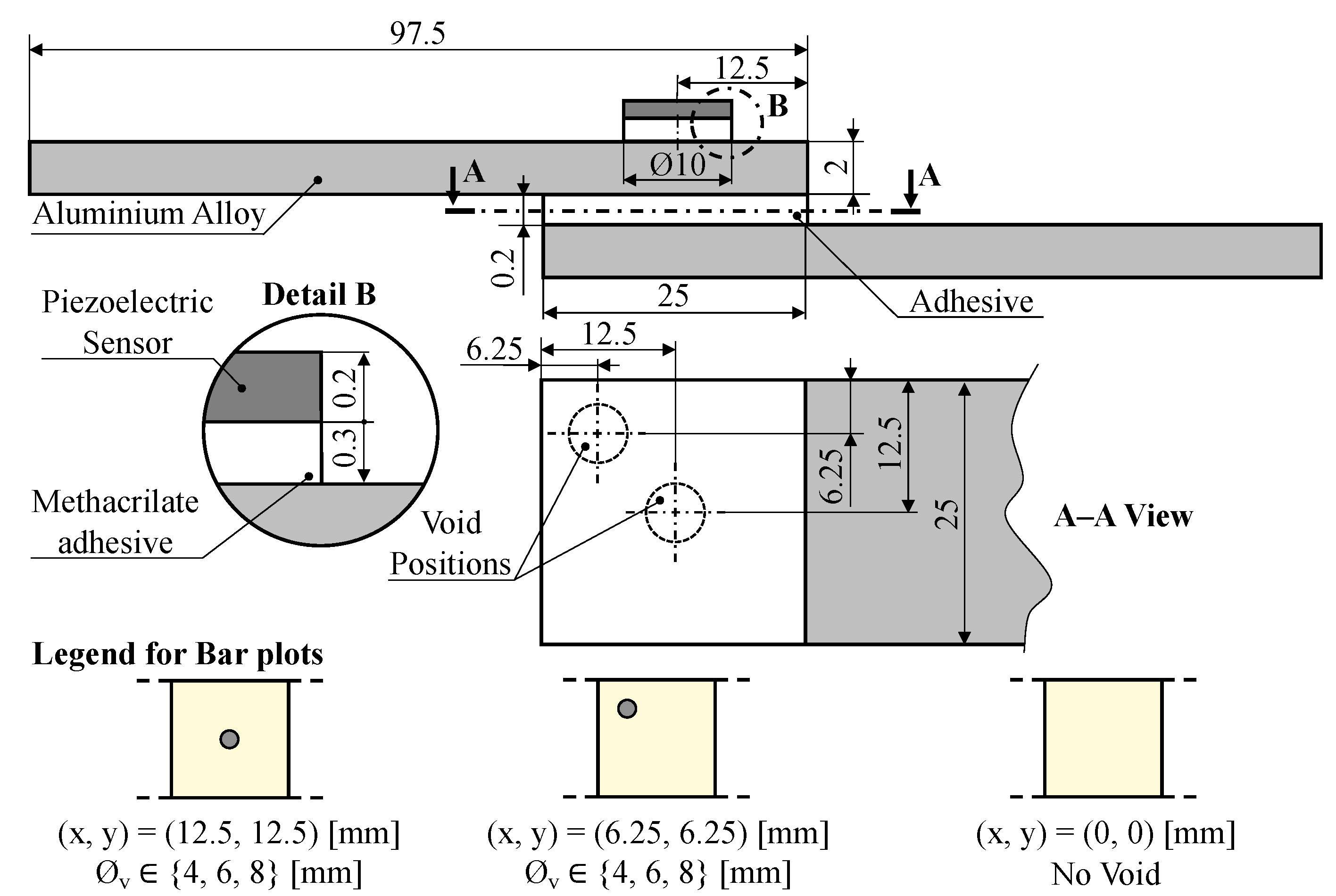


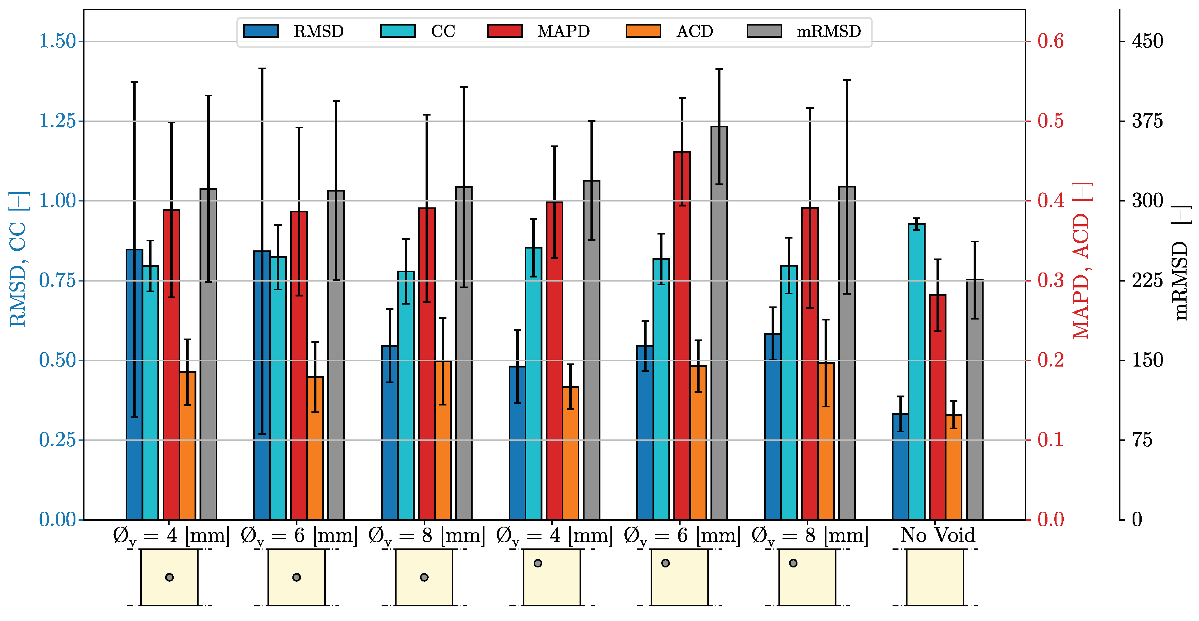
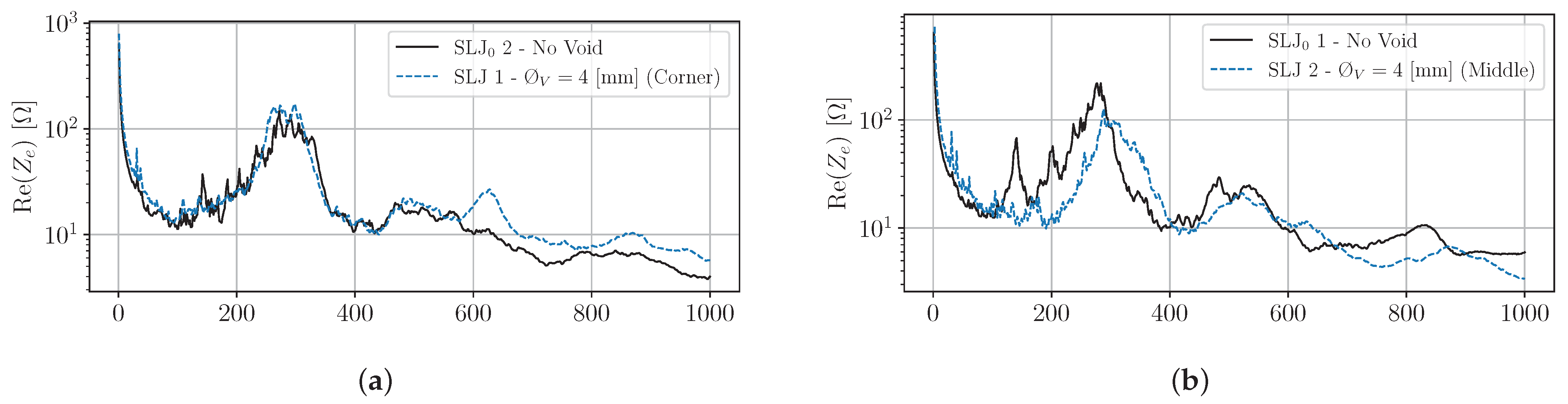

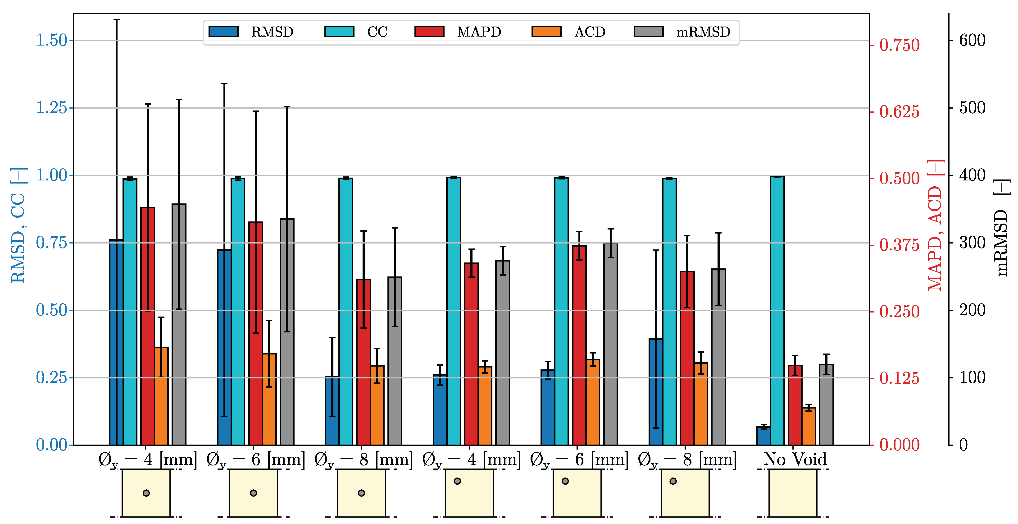

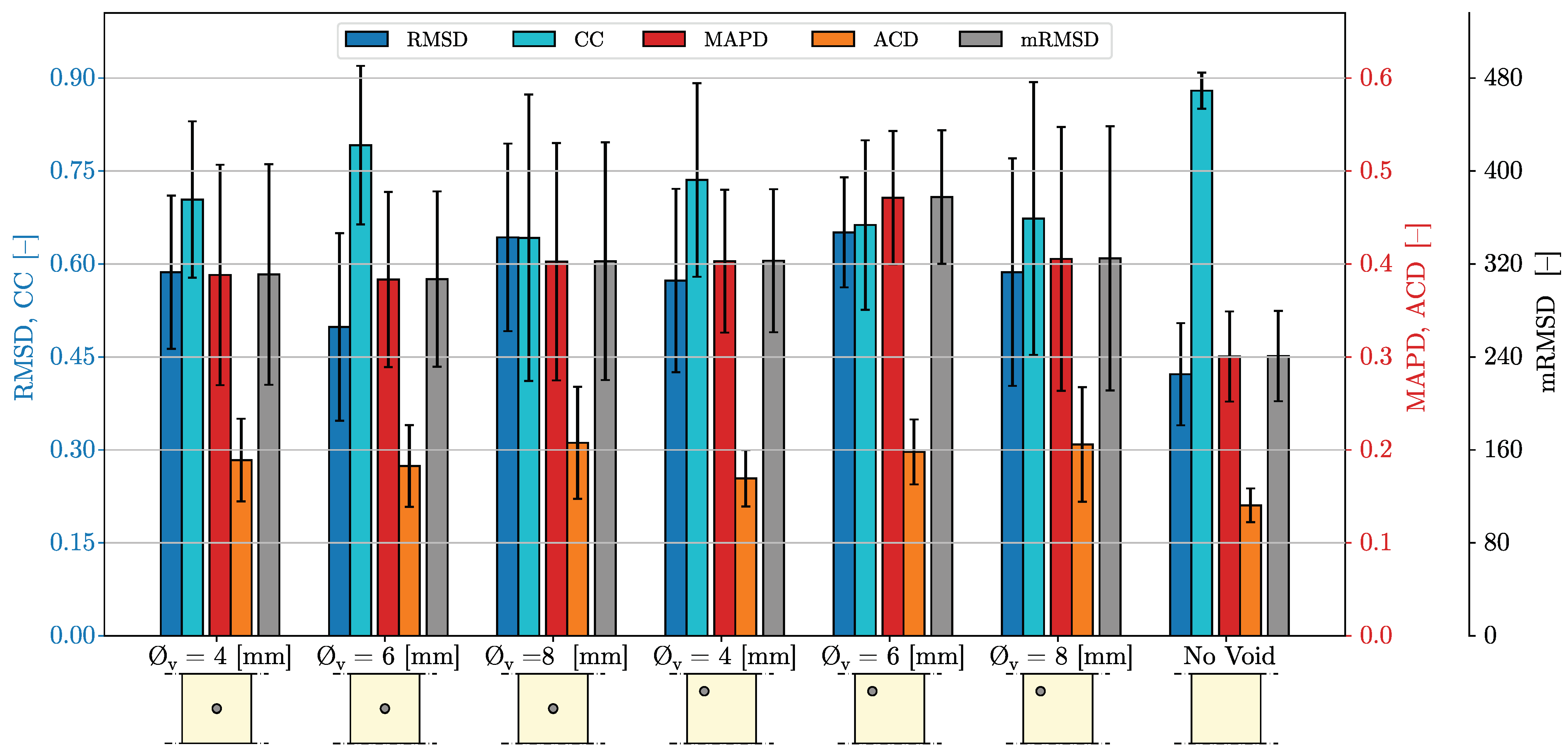

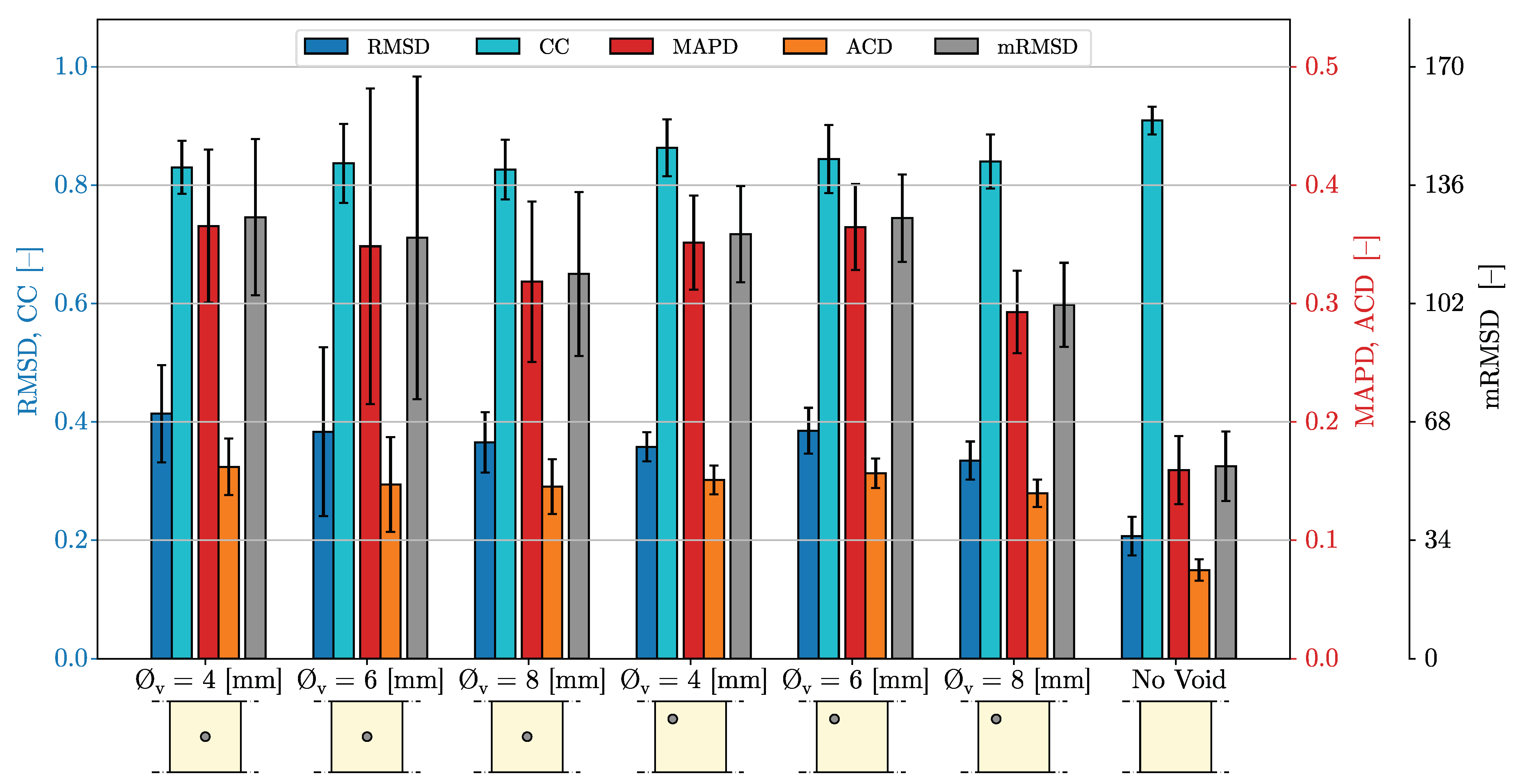

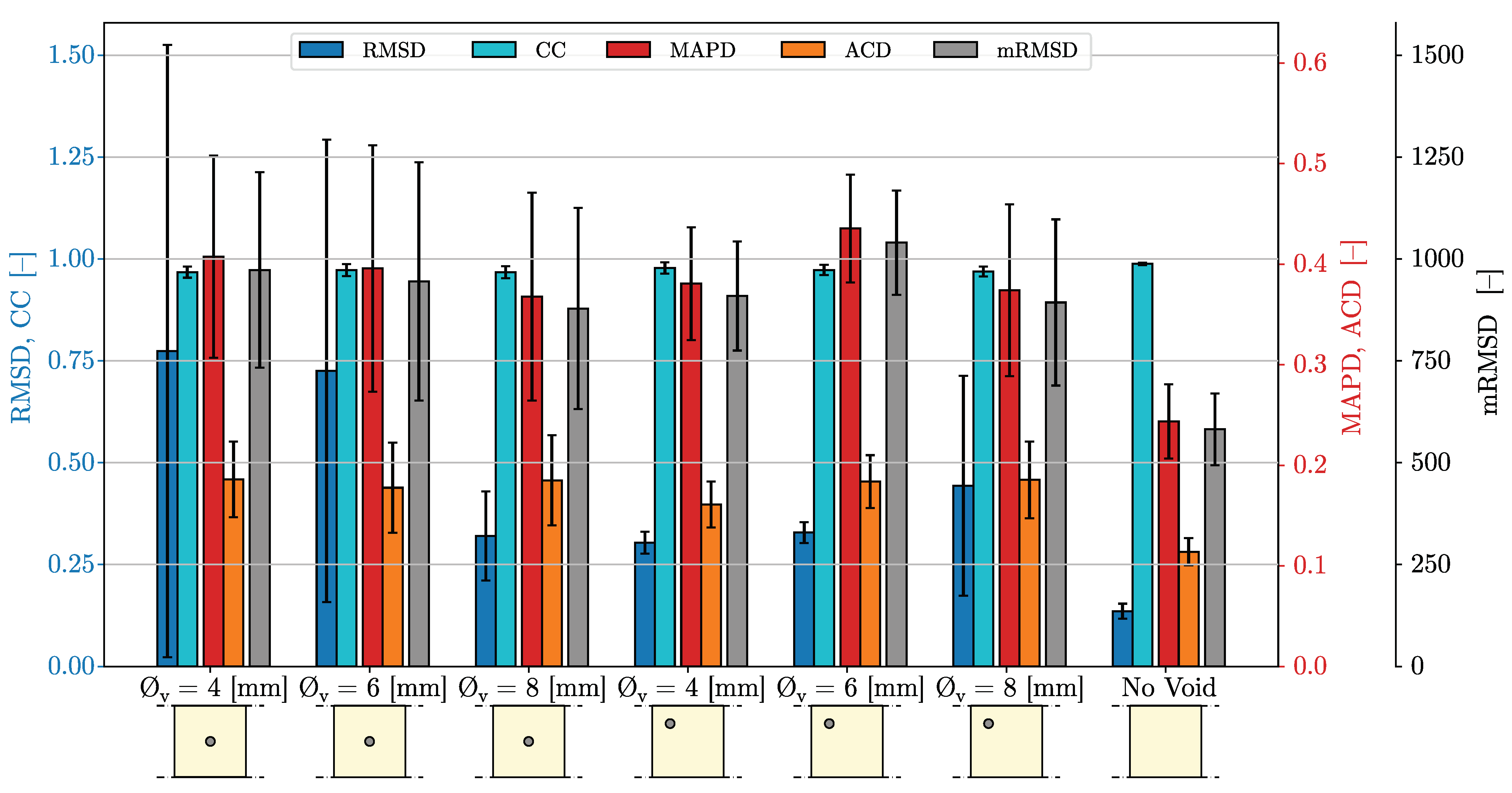
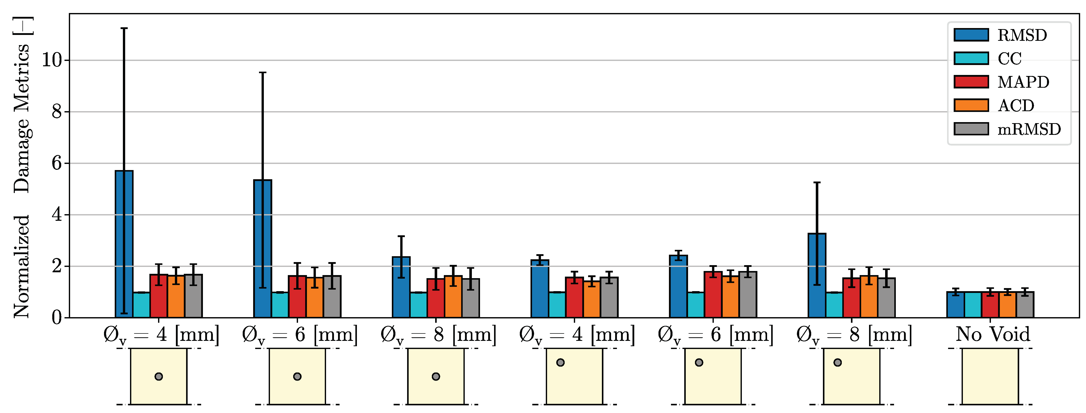

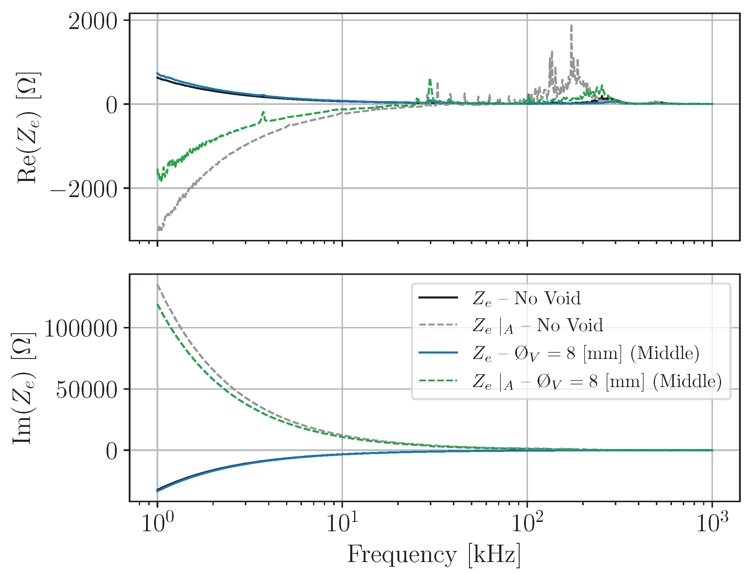
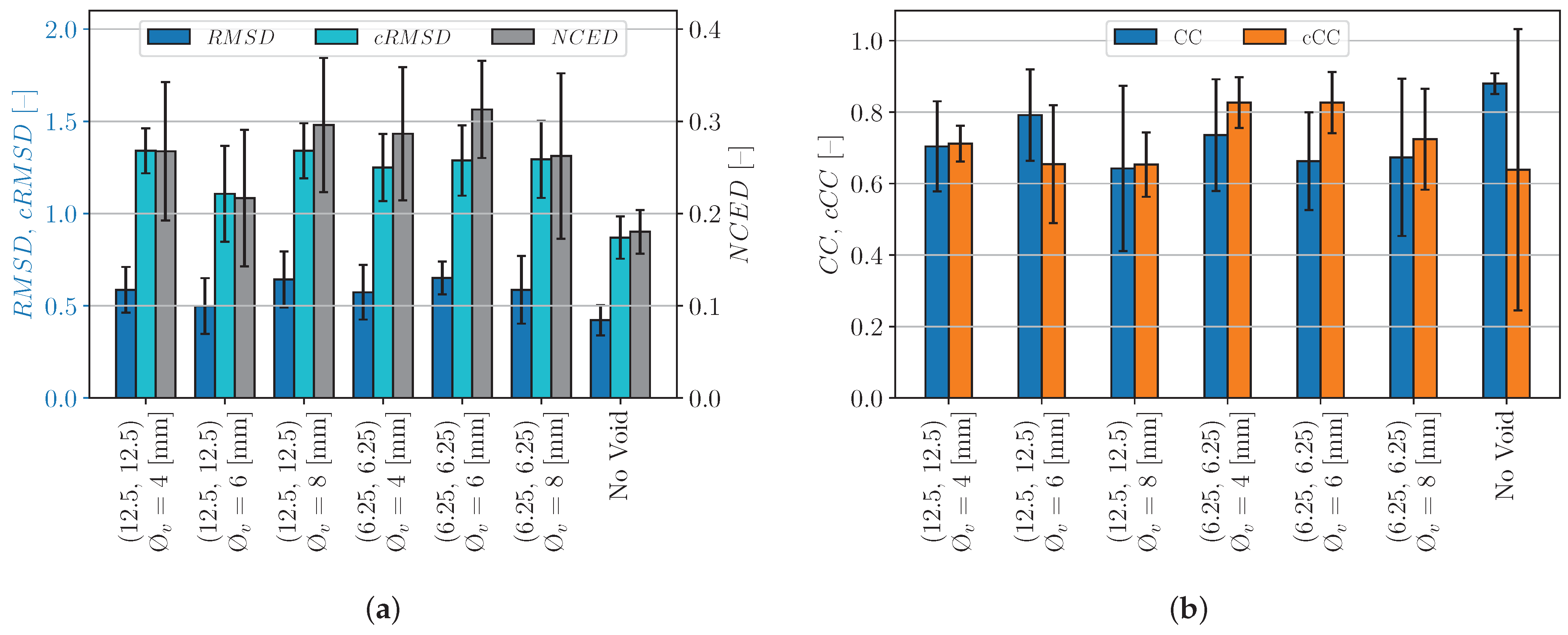
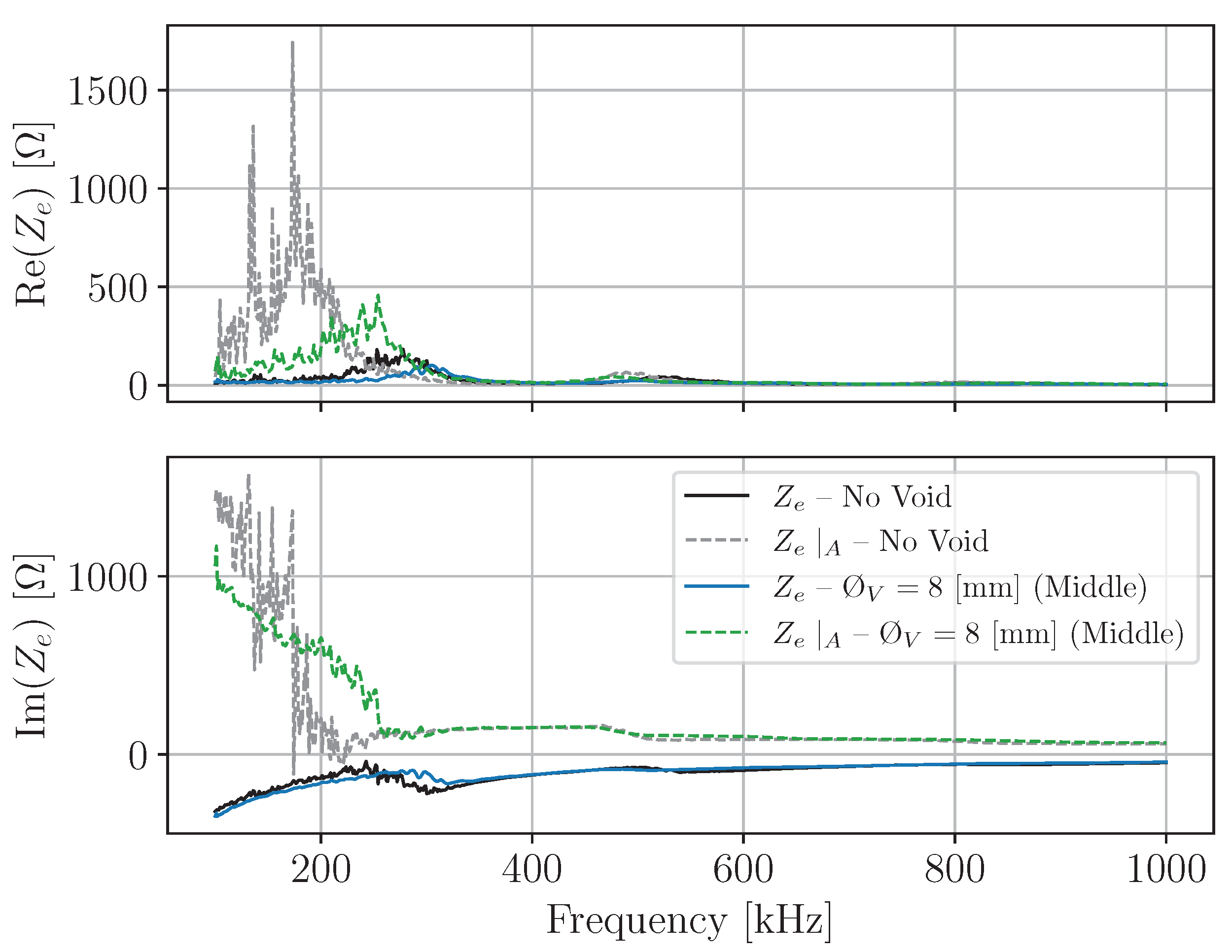


Disclaimer/Publisher’s Note: The statements, opinions and data contained in all publications are solely those of the individual author(s) and contributor(s) and not of MDPI and/or the editor(s). MDPI and/or the editor(s) disclaim responsibility for any injury to people or property resulting from any ideas, methods, instructions or products referred to in the content. |
© 2023 by the authors. Licensee MDPI, Basel, Switzerland. This article is an open access article distributed under the terms and conditions of the Creative Commons Attribution (CC BY) license (https://creativecommons.org/licenses/by/4.0/).