Abstract
Overlapping coefficients (OVL) are commonly used to estimate the similarity between populations in terms of their density functions. In this paper, we consider Pianka’s overlap coefficient for two exponential populations. The methods for statistical inference of Pianka’s coefficient are presented. The bias and mean square error (MSE) of the maximum likelihood estimator (MLE) and the Bayes estimator of Pianka’s overlap coefficient are investigated by simulation. Confidence intervals for Pianka’s overlap measure are constructed.
Keywords:
overlapping measure; maximum likelihood estimator; limiting distribution; posterior distribution; Bayes estimator; multivariate delta method; exponential distribution MSC:
62F10; 62F12
1. Introduction
Overlapping coefficients (OVL) are measures of how similar two populations are; this similarity is a function that assigns a real number between 0 and 1, where a value of zero indicates that the distributions are completely different and a value of one indicates that they are identical. There are many overlapping coefficients in the literature, including measures of overlap that determine the percentage of area that the two distributions have in common [1]. Gini and Livada [2] first introduced the idea of overlapping in 1943. Matusita’s coefficient [3] was introduced to calculate the significant distance between two probability density functions, and has applications in several practical areas, including reliability analysis and clinical research [4,5]. Matusita developed a discrete version known as the Freeman–Tukey (FT) measure, which is related to the Hellinger distance [6,7] and the delta method [8]. The Chi-Squared measure [9] and Hellinger measure [10] play key roles in information theory, statistics, learning, signal processing, and other theoretical and applied branches of mathematics [11,12]. Morisita’s coefficient [13] was proposed as an index of similarity between two communities. Weitzman’s coefficient [14], primarily used to compare income distributions, was defined as the region where the curves of two probability distributions intersect. Kullback and Leibler [15] introduced the Kullback–Leibler measure, which measures the gain in information between two distributions and has been widely used in the literature on data mining. Jeffreys [16] introduced and studied a divergence measure called the Jeffreys distance, which is regarded as a symmetrization of the Kullback–Leibler measure. For a comprehensive review of various divergence measures, see [17,18,19].
The OVL coefficients are used in various fields, such as ecological processes [20], statistical ecology [21], clinical trials [5], data fusion [22], information processing [23], applied statistics [24], economics [25], and others.
Inference for OVL measures has been investigated by several researchers under normal, Weibull, and exponential distributions. In 2005, al-Saidy et al. [26] presented the inference of three OVL coefficients for two Weibull distributions with the same shape parameter and different scale parameters.
Al-Saleh and Samawi [27] used bootstrap and Taylor series approximation to investigate the interval estimation of three OVL coefficients for two exponential distributions with different means. Samawi and Al-Saleh [28] studied three OVL coefficients for two exponential distributions and estimated them using ranked set sampling. Hamza et al. [29] proposed a new OVL coefficient based on the Kullback–Leibler measure for two exponential distributions. Sibil et al. [30] investigated both interval estimation and hypothesis testing for the OVL coefficients for one- and two-parameter exponential distributions using the concept of a generalized pivotal quantity.
Pianka’s overlap coefficient is used to assess the similarity of resource use by two species [31], they used Pianka’s overlap coefficient as a summary measure and to make inferences, typically about competition for resources.
Pianka’s overlap is used in mechanisms that favour morphological co-occurrence; Vieira and Port [32] evaluated the Pianka’s overlap between two species based on three main niche dimensions: habitat, food, and time. Jacqueline et al. [33] calculated dietary overlap between foxes and dingoes using Pianka’s index. Sa Oliveira et al. [34] investigated diet and niche breadth in fish communities, for which they estimated niche breadth using the liven index and Pianka’s measure.
In this paper, we consider the Pianka’s OVL coefficient () between two exponential distributions. We determine both the limiting and exact distributions for the maximum likelihood estimator (MLE) of . We study the MLE and Bayesian estimators and compare their efficiency with each other. In addition, we consider interval estimation of using the asymptotic technique and the transformation technique, and compare the effectiveness of both techniques.
2. General Setting and Definition of the Pianka Overlap Measure
Let and be two continuous probability density functions. Pianka’s overlap measure is defined as follows [31]:
If a random variable X follows the exponential distribution, then the respective cdf and pdf of X are provided by
and X is denoted by .
Now, let and be two independent random samples taken from and , respectively. Then, the Pianka’s overlap coefficient between the two exponential distributions, as defined in Equation (1), is provided by
Let . Then, the Pianka’s OVL coefficient in (2) can be written as a function of k, as follows:
Several properties of are provided in the following lemma.
Lemma 1.
For ρ defined in (3):
- 1.
- for all
- 2.
- iff i.e.,
- 3.
- , since
- 4.
- 5.
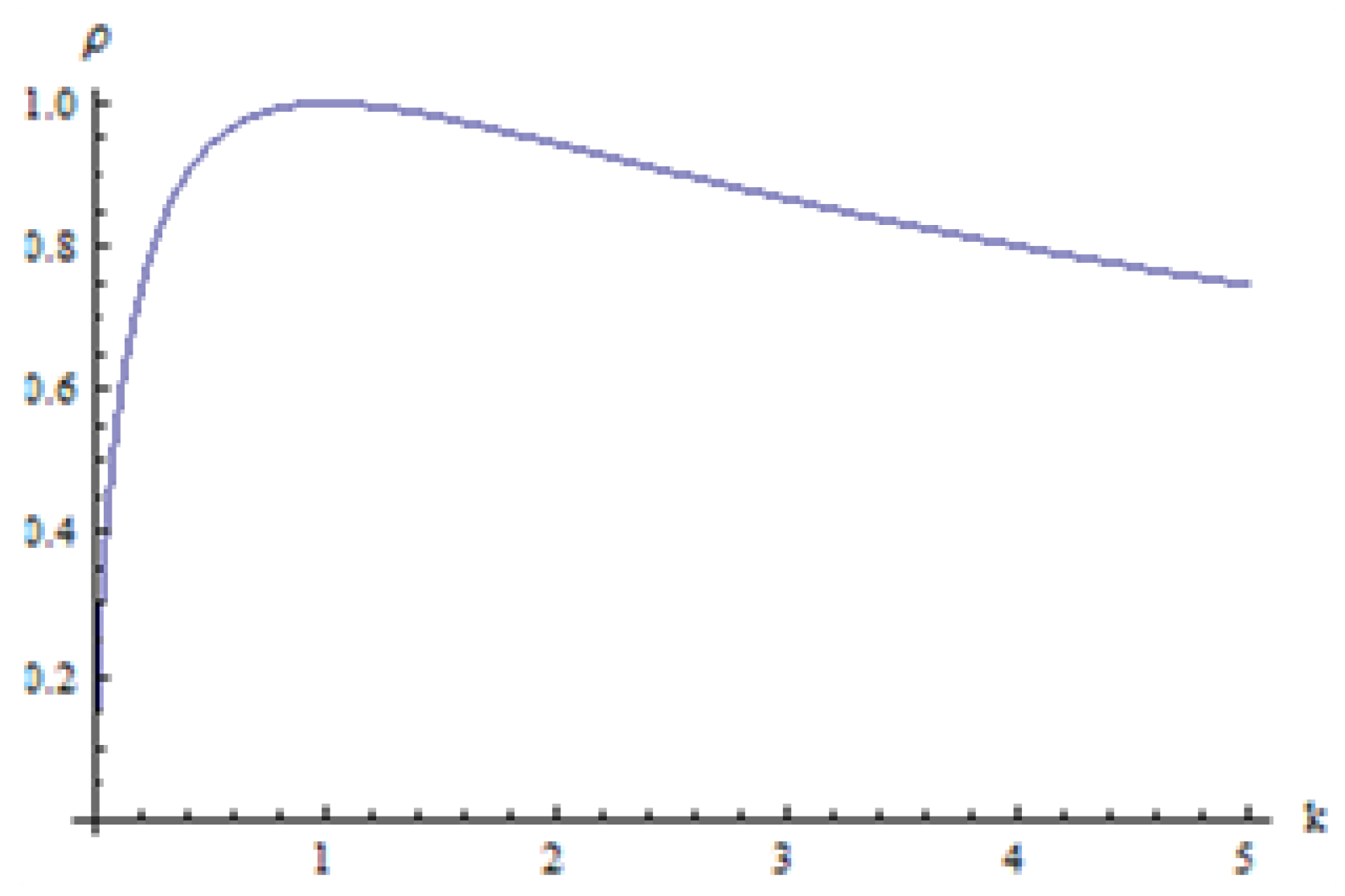
- is monotonically increasing for and decreasing for with a maximum of at
Proof.
It is easy to derive the above results from the formula of the Pianka’s overlap coefficient formula in (3). □
Figure 1 shows the plot of the Pianka’s overlap coefficient between two exponential distributions as a function of k, where
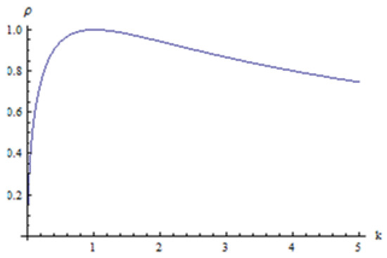
Figure 1.
Pianka overlap coefficient as a function of k.
In the following section, we find the maximum likelihood estimator of Pianka’s overlap coefficient , namely, , along with its distribution. In addition, we investigate the limiting distribution of .
3. Maximum Likelihood Estimator of
It is known that the MLEs for and based on two samples taken from and are provided by and , respectively. From the basic properties of the exponential distribution, we have with and and with , where stands for the gamma distribution with shape parameter and scale parameter . It follows that the estimates represent a complete minimal sufficient statistic for . Thus, from the invariance property of the MLE, the MLE of is
3.1. Limiting Distribution of
The following theorem concludes that the limiting distribution for the MLE of Pianka’s overlap coefficient for two exponential distributions with different scale parameters is the normal distribution, using to denote the normal distribution with location parameter and scale parameter .
Theorem 1.
Let and be two independent random samples from and respectively, with Then, the asymptotic distribution for is
Proof.
Using the asymptotic property of MLE and the multivariate delta method (δ−method), we have
That is,
where is the Fisher information.
We want to find the asymptotic distribution of as
Using the fact that and and the continuous mapping theorem, we obtain
Now, we are interested in the asymptotic distribution of
Because is a function of and using an alternative form of the multivariate δ−method [35] we obtain and
Therefore, the asymptotic distribution of is
□
3.2. The Exact Distribution of
To ease the derivation of the distribution of we can rewrite Equation (4) as follows:
where and . Now, we apply the following steps.
- Step 1.
- Find the pdf of by considering the following transformations.Let and ; then, and The absolute value of the Jacobian of this transform isThus, the joint pdf of and isBy integrating out, the pdf of isConsequently, the pdf of H iswhere
- Step 2.
- Solve forFrom Equation (5) and the transformation , we haveNow, let , allowing to be rewritten as the quadratic equationThe two solutions of Equation (6) areand
- Step 3.
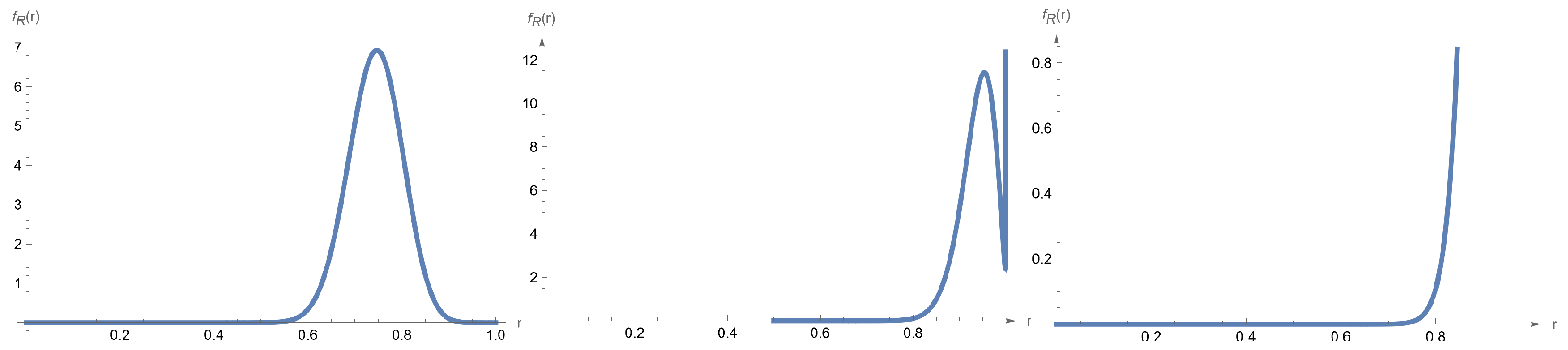
- The pdf of isFigure 2 shows different plots of the density of for . Based on the figure, the pdf of can be bell-shape, bimodal, or J-shaped.
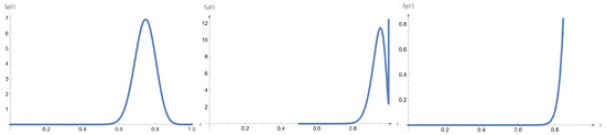 Figure 2. The pdf of for ) = (2,10), (5,10), and (8,10).
4. Interval Estimation of
In this section, we find interval estimation of Pianka’s overlap coefficient by considering both asymptotic and transformation techniques; later, in Section 6, we perform a Monte Carlo analysis to compare the effectiveness of these two different approaches.
4.1. Asymptotic Technique
A large sample confidence interval for can be easily calculated. From theorem (2.1) and the continuous mapping theorem, we have
Hence, a large sample confidence interval for is
where is the γth percentile of the standard normal distribution.
4.2. Transformation Technique
From the assumption in Equation (3), , where the MLE of k is . From Section 3 and the relationship between the gamma distribution and the chi-square distribution, it is easy to conclude that and ; thus, has an F-distribution with degrees of freedom.
Let L and U be the lower and upper confidence limits, respectively; from the concept of the confidence interval, we have
However, the overlap coefficient is not a monotone function of k. Therefore, using the transformation technique, we can obtain a confidence interval for , as follows:
where is the percentile of the F−distribution with degrees of freedom.
5. Bayes Estimator of
Let and be two independent random samples taken from and , respectively. Let , and where is the inverse gamma distribution.
Using the fact that and , the posterior distribution of given is
where and are prior probability distributions for and , respectively.
Then,
where and
The Bayes estimator is
The above estimate does not have a simple closed form; thus, we obtain it numerically. For the asymptotic distribution of the Bayes estimator , the Bernstein–von Misses theorem [36] concludes that the Bayesian estimator and the maximum likelihood estimator are asymptotically equivalent for large sample sizes.
In the next section, we present a simulation study to compare the two approaches for finding the interval estimator of Pianka’s overlap coefficient, as described earlier in Section 4. Additionally, we investigate the performance of the maximum likelihood estimator ( and Bayes estimator ( of the Pianka’s overlap coefficient detailed in Section 3 and Section 5.
6. Simulation Study
To compare the two approaches of interval estimation of Pianka’s overlap coefficient, we consider two criteria:
- 1.
- The term “valid confidence level” can be applied to an interval estimation process when, in repeated sampling, the actual coverage of the true but unmeasured statistic is close to the nominal confidence level;
- 2.
- If the expected length of the simulated period is short, a method for estimating intervals can be described as “valid length-efficient”.
To compare the estimators, we use the bias, mean square error (MSE), and efficiency for each estimator. In order to use the above criteria, we conducted a simulation study, as follows:
- 1.
- A random sample of size n is generated from This random sample is used to calculate
- 2.
- A random sample of size m is generated from This random sample is used to calculate
- 3.
- The lower limit upper limit , and width are calculated with a nominal confidence level of .
- 4.
- The MLE and the Bayes ( estimators are calculated.
- 5.
- Steps 1–4 above are repeated 10,000 times.
- 6.
- The average of the lower limits (AL), median of the lower limits (ML), average of the upper limits (AU), median of the upper limits (MU), average width (AW), and median width (MW) are calculated for each interval.
- 7.
- The percentage of out of the 10,000 samples generated in Step 3 is called the “coverage probability” and is denoted by .
- 8.
- Histogram Plots for and are generated.
- 9.
- Bias and MSE are calculated for and , then efficiency is calculated
- 10.
- Steps 1–9 above are repeated forandfor each value of
Mathematica was used to simulate each of the interval estimation and point estimation methods for the Pianka’s overlap measure .
Table 1, Table 2 and Table 3 show the simulated interval estimators using the asymptotic and transformation techniques based on exponential random samples with a nominal confidence level of . These results show that the average width (AW) is almost the same as the median width (MW) and that the transformation method consistently performs better in terms of the confidence interval width. Moreover, the transformation method appears to be effective in terms of the coverage probability except for values of k around one and very small sample sizes.

Table 1.
Simulation results for the two approaches of interval estimation of Pianka’s OVL coefficient for .
Table 2.
Simulation results for the two approaches of interval estimation of Pianka’s OVL coefficient for .
Table 3.
Simulation results fir the two approaches of interval estimation of Pianka’s OVL coefficient for .
As the sample size increases, the coverage probability of the two techniques approaches the nominal value. The coverage probability of the asymptotic technique works very well, and increases as k approaches one; however, when and for small sample sizes the transformation technique performs exceptionally well.
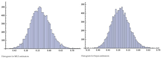
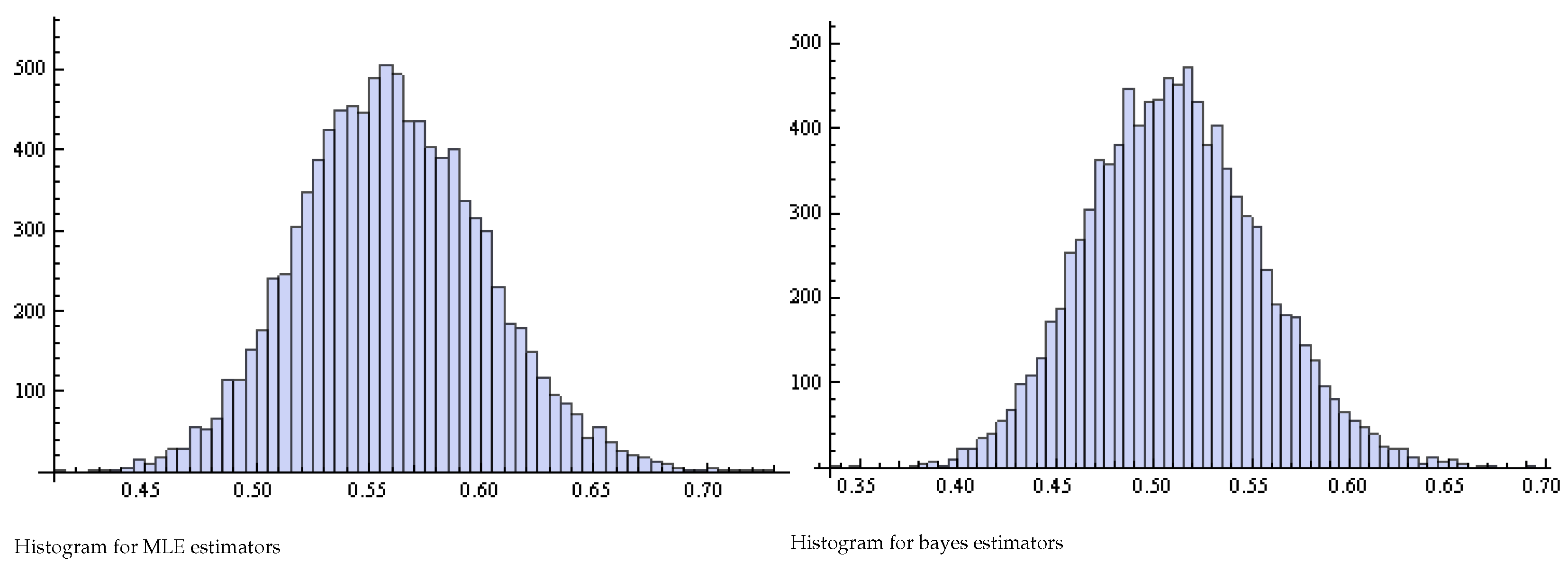
Figure 3.
Histogram of Pianka estimators for and .
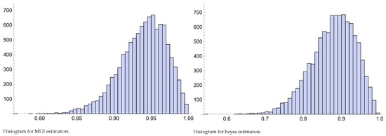
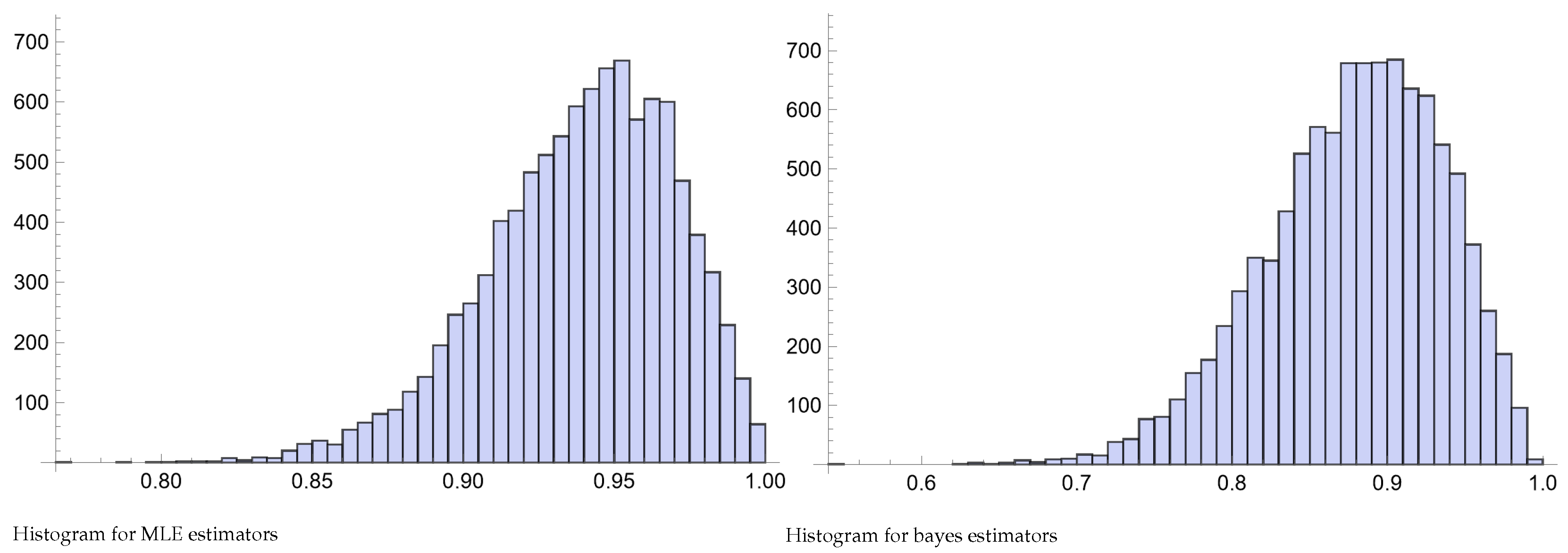
Figure 4.
Histogram of Pianka estimators for and .
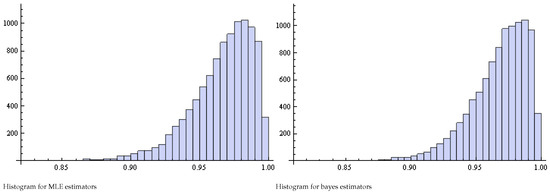
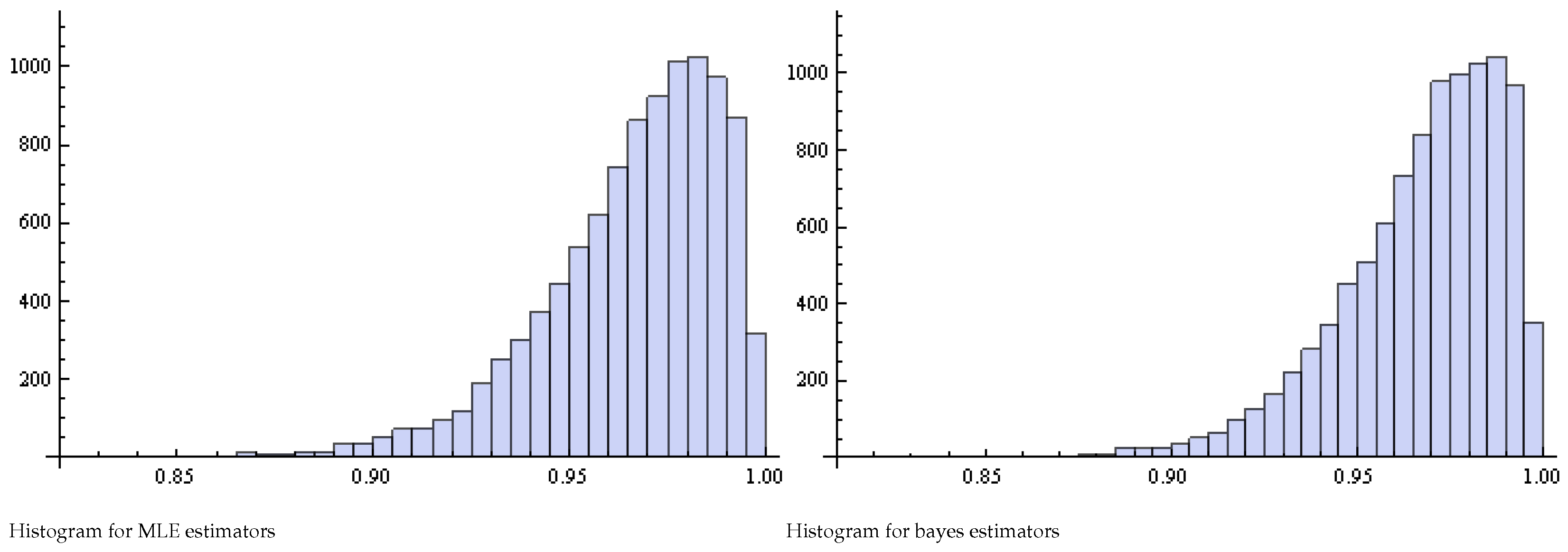
Figure 5.
Histogram of Pianka estimators for and .
Table 4, Table 5 and Table 6 present the results of the simulation study carried out to compare the MLE and Bayes estimators for the Pianka’s overlap coefficient. Based on these results, which only consider the values of the absolute values of the bias are in all cases less than and decrease as the sample size increases. It appears that the MLE estimator works well, and the Bayes estimator seems to work quite well at However, for the calculations are provided in terms of for the Pianka’s overlap measure. For sample sizes larger than 30, the bias and MSE are quite close to zero.
Table 4.
Bias, MSE, and efficiency of the two estimators of Pianka’s OVL coefficient for . Exact Pianka’s coefficient .
Table 5.
Bias, MSE, and efficiency of the two estimators of Pianka’s OVL coefficient for Exact Pianka’s coefficient .
Table 6.
Bias, MSE, and efficiency of the two estimators of Pianka’s OVL coefficient for . Exact Pianka’s coefficient .
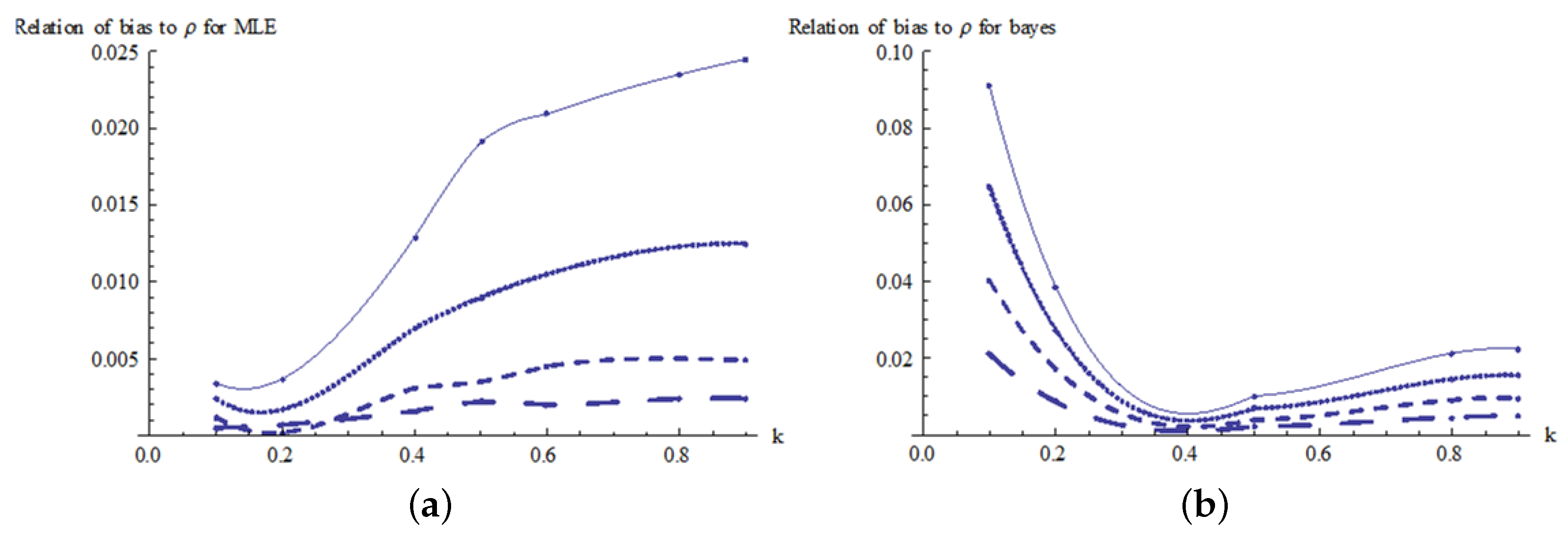
The estimates of the bias are plotted in Figure 6 for the MLE and Bayes estimators. From these results, it can be seen that the bias decreases significantly as the sample size increases. Figure 6a shows that the actual Pianka’s overlap is underestimated; however, for very small values of k and small sample sizes the true Pianka’s overlap is overestimated. Furthermore, the bias increases as k increases for the MLE estimator.
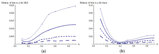
Figure 6.
Relationship of bias to k for Pianka’s coefficient: (a) relation of bias to for the MLE estimator and (b) relation of bias to for the Bayes estimator.
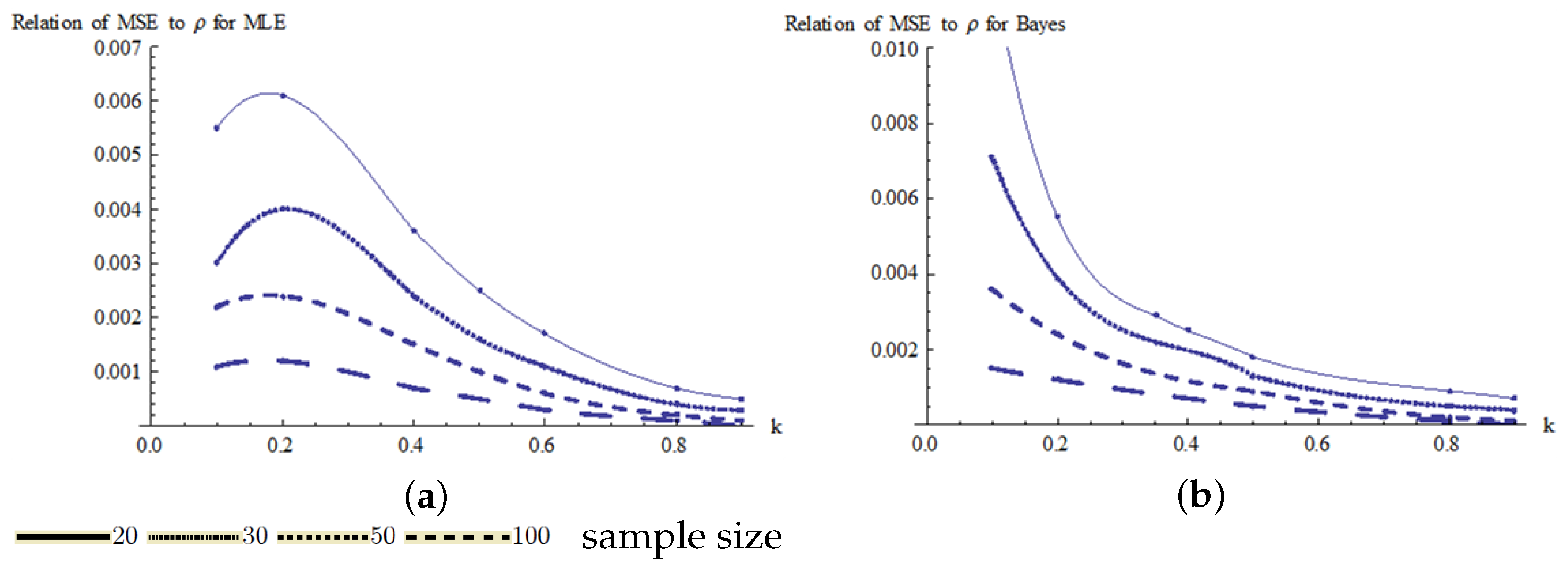
The estimates of MSE are plotted in Figure 7 for the MLE and Bayes estimators. From these results, it can be seen that the MSE decreases significantly as the sample size increases. Figure 7a shows that for small k values and small sample sizes, there is a significant increase in the MSE for the MLE estimator. For the Bayes estimator, Figure 6b and Figure 7b show that both the bias and the MSE decrease as the value of k increases.
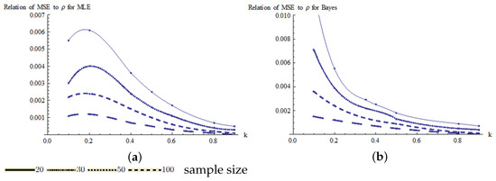
Figure 7.
Relationship of MSE to k for Pianka’s coefficient: (a) relation of MSE to for the MLE estimator and (b) relation of bias to for Bayes estimator.
7. Conclusions
We have estimated Pianka’s overlap coefficient for two exponential populations with different scale parameters using the MLE and Bayes estimators, then compared these estimators by calculating the bias and MSE in a simulation study. In addition, we have constructed confidence intervals for the Pianka’s overlap measure using asymptotic and transformation techniques, then compared them using the “valid confidence level” and “valid length-efficiency”.
We investigated the accuracy of the Pianka’s overlap coefficient through a Monte Carlo analysis. In conclusion, it appears that there is no ideal approach. Therefore, a transformation procedure is recommended when and the sample size is small. The asymptotic approach can be used if computers are available. For larger sample sizes and , the transformation approach is recommended.
Author Contributions
Conceptualization, S.A. and M.A.; Methodology, S.A. and M.A.; Software, S.A. and M.A.; Validation, S.A. and M.A.; Formal analysis, S.A. and M.A.; Resources, S.A. and M.A.; Writing—original draft, S.A.; Writing—review & editing, M.A. All authors have read and agreed to the published version of the manuscript.
Funding
This research received no external funding.
Data Availability Statement
Not applicable.
Conflicts of Interest
The authors declare no conflict of interest.
References
- Tilton, J.W. The measurement of overlapping. J. Educ. Psychol. 1937, 28, 656–662. [Google Scholar] [CrossRef]
- Gini, C.; Livada, G. Nuovi Contribute Alla Teoria Della Transvariazione; Atti della VI Riunione della Società Italiana di Statistica: Rome, Italy, 1943. [Google Scholar]
- Matusita, K. Decision rules based on distance, for problems of fit, two samples and applications. Ann. Inst. Math. Stat. 1955, 19, 181–192. [Google Scholar] [CrossRef]
- Anderson, G. Toward an empirical analysis of polarization. J. Econom. 2004, 122, 1–26. [Google Scholar] [CrossRef]
- Mizuno, S.; Yamaquchi, T.; Fukushima, A.; Matsuyama, Y.; Ohashi, Y. Overlap coefficient for assessing the similarity of pharmacokinetic data between ethnically different populations. Clin. Trials 2005, 2, 174–181. [Google Scholar] [CrossRef]
- Beran, R. Minimum Hellinger distance estimates for parametric models. Ann. Stat. 1977, 5, 455–463. [Google Scholar] [CrossRef]
- Rao, K.J.N.; Tintner, G. On the variate difference method. Aust. J. Stat. 1963, 5, 106–116. [Google Scholar] [CrossRef]
- Smith, E.P. Niche breadth, resource availability, and inference. Ecology 1982, 63, 1675–1681. [Google Scholar] [CrossRef]
- Pearson, K. On the Criterion that a Given System of Deviations From the Probable in the Case of a Correlated System of Variables is such that it Can be Reasonably Supposed to have a Risen From Random Sampling. Lond. Edinb. Dublin Philos. Mag. J. Sci. 1991, 50, 157–172. [Google Scholar] [CrossRef]
- Hellinger, E. Neue begründung der theorie quadratischer formen von unendlichvielen veränderlichen. J. Reine Angew. Math. 1909, 136, 210–271. [Google Scholar] [CrossRef]
- Nishiyama, T. A tight lower bound for the Hellinger distance with given means and variances. arXiv 2020, arXiv:2010.13548. [Google Scholar]
- Nishiyama, T.; Sason, I. On relations between the relative entropy and χ2-divergence, generalizations and applications. Entropy 2020, 22, 563. [Google Scholar] [CrossRef]
- Morisita, M. Measuring of the dispersion and analysis of distribution patterns, Memoires of the Faculty of Science, Series E. Biol. Kyushu Univ. 1959, 2, 215–235. [Google Scholar]
- Weitzman, M.S. Measures of overlap of income distributions of white and Negro families in the United States. In US Bureau of the Census; U.S. Department of Commerce: Washington, DC, USA, 1970; Volume 22. [Google Scholar]
- Kullback, S.; Leibler, R.A. On information and sufficiency. Ann. Math. Stat. 1951, 22, 79–86. [Google Scholar] [CrossRef]
- Jeffreys, H. An invariant form for the prior probability in estimation problems. Proc. R. Soc. Lond. Ser. A Math. Phys. Sci. 1946, 186, 453–461. [Google Scholar]
- Abu, A.H.; Hassanat, A.; Lasassmeh, O.; Tarawneh, A.; Alhasanat, M.; Eyal, S.H.; Prasath, V. Effects of distance measure choice on k-nearest neighbor classifier performance: A review. Big Data 2019, 7, 221–248. [Google Scholar]
- Cha, S. Comprehensive survey on distance/similarity measures between probability density functions. City 2007, 1, 1. [Google Scholar]
- Taneja, I. On symmetric and nonsymmetric divergence measures and their generalizations. Adv. Imaging Electron Phys. 2005, 138, 177–250. [Google Scholar]
- Abele, L.G. The community structure of coral-associated decapod crustaceans in a variable environment. Ecol. Process. Coast. Mar. Syst. Mar. Sci. 1979, 10, 265–287. [Google Scholar]
- Chao, A.; Hwang, W.; Chen, Y.; Kuo, C. Estimating the number of shared species in two communities. Stat. Sin. 2000, 10, 227–246. [Google Scholar]
- Moravec, H. Mind Children: The Future of Robot and Human Intelligence; Harvard University Press: Cambridge, MA, USA, 1988. [Google Scholar]
- Viola, P.; Wells, W., III. Alignment by maximization of mutual information. Int. J. Comput. Vis. 1997, 24, 137–154. [Google Scholar] [CrossRef]
- Inman, H.F.; Bradley, E.L. The overlapping coefficient as a measure of agreement between probability distributions and point estimation of the overlap of two normal densities. Commun. Stat. Theory Methods 1989, 18, 3851–3874. [Google Scholar] [CrossRef]
- Milanovic, B.; Shlomo, Y. Decomposing world income distribution: Does the world have a middle class? Rev. Income Wealth 2002, 48, 155–178. [Google Scholar] [CrossRef]
- Al-Saidy, O.; Samawi, H.M.; Al-Saleh, M.F. Inference on overlap coefficients under the Weibul distribution: Equal Shape Parameter. ESAIM Probab. Stat. 2005, 9, 206–219. [Google Scholar] [CrossRef]
- Al-Saleh, M.F.O.; Samawi, H. Interference on Overlapping Coefficients in Two Exponential Populations. J. Mod. Appl. Stat. Methods 2007, 6, 503–516. [Google Scholar] [CrossRef]
- Samawi, H.; Al-Saleh, M.F.O. Inference on Overlapping Coefficients in Two Exponential Populations Using Ranked Set Sample. Commun. Korean Stat. Soc. 2008, 15, 147–159. [Google Scholar]
- Hamza, D.; Papa, N.; Malick, M. Overlap Coefficients Based on Kullback-Leibler Divergence: Exponential Populations Case. Int. J. Appl. Math. Res. 2017, 6, 135–140. [Google Scholar]
- Sibil, J.; Seemon, T.; Thomas, M. Interval Estimation of the Overlapping Coefficient of Two Exponential Distributions. J. Stat. Theory Appl. 2019, 18, 26–32. [Google Scholar]
- Pianka, E. Niche Overlap and Diffuse Competition. Proc. Natl. Acad. Sci. USA 1974, 71, 2141–2145. [Google Scholar] [CrossRef]
- Vieira, E.M.; Port, D. Niche overlap and resource partitioning between two sympatric fox species in southern Brazil. J. Zool. 2006, 272, 57–63. [Google Scholar] [CrossRef]
- Jacqueline, B.C.; Mathew, S.C.; Georgeanna, S.; Mike, L. Dietary overlap and prey selectivity among sympatric carnivores: Could dingoes suppress foxes through competition for prey? J. Mammal. 2011, 92, 590–600. [Google Scholar]
- Sa-Oliveira, J.C.; Ronaldo, A.; Victoria, J.I.N. Diet and niche breadth and overlap in fish communities within the area affected by an Amazonian reservoir (Amapá, Brazil). Ann. Braz. Acad. Sci. 2014, 86, 383–405. [Google Scholar] [CrossRef] [PubMed]
- Bodkin, R.G.; Klein, L.R.; Marwah, K. A History of Macroeconometric Model-Building; Edward Elgar Publishing: Cheltenham, UK, 1991. [Google Scholar]
- Doob, J. Application of the theory of martingales. Calc. Des Probab. Ses Appl. 1949, 13, 23–27. [Google Scholar]
Disclaimer/Publisher’s Note: The statements, opinions and data contained in all publications are solely those of the individual author(s) and contributor(s) and not of MDPI and/or the editor(s). MDPI and/or the editor(s) disclaim responsibility for any injury to people or property resulting from any ideas, methods, instructions or products referred to in the content. |
© 2023 by the authors. Licensee MDPI, Basel, Switzerland. This article is an open access article distributed under the terms and conditions of the Creative Commons Attribution (CC BY) license (https://creativecommons.org/licenses/by/4.0/).