Efficient Monitoring of a Parameter of Non-Normal Process Using a Robust Efficient Control Chart: A Comparative Study

Abstract

The control chart is a fundamental tool in statistical process control (SPC), widely employed in manufacturing and construction industries for process monitoring with the primary objective of maintaining quality standards and improving operational efficiency. Control charts play a crucial role in identifying special cause variations and guiding the process back to statistical control. While Shewhart control charts excel at detecting significant shifts, EWMA and CUSUM charts are better suited for detecting smaller to moderate shifts. However, the effectiveness of all these control charts is compromised when the underlying distribution deviates from normality. In response to this challenge, this study introduces a robust mixed EWMA-CUSUM control chart tailored for monitoring processes characterized via symmetric but non-normal distributions. The key innovation of the proposed approach lies in the integration of a robust estimator, based on order statistics, that leverages the generalized least square (GLS) technique developed by Lloyd. This integration enhances the chart’s robustness and minimizes estimator variance, even in the presence of non-normality. To demonstrate the effectiveness of the proposed control chart, a comprehensive comparison is conducted with several well-known control charts. Results of the study clearly show that the proposed chart exhibits superior sensitivity to small and moderate shifts in process parameters when compared to its predecessors. Through a compelling illustrative example, a real-life application of the enhanced performance of the proposed control chart is provided in comparison to existing alternatives.

1. Introduction

There is no production or manufacturing process which does not contain some amount of variation. In any production or manufacturing process, this amount of variation is categorized into two general categories, natural cause variation and assignable cause variation. Natural cause variation is also known as common cause variation and assignable cause variation is also considered as special cause variation. Even with the use of precise instruments, a controlled working environment, and monitoring the external factors that may influence the output, one cannot completely eliminate natural cause variations. A process is said to be statically in-control even in the presence of natural cause variations. This means we have to live with these variations no matter what we do to keep them away from the production or manufacturing process. On the other hand, the variations that can be controlled or minimized by careful inspection of the production process are considered as assignable cause variations. Process is considered as out-of-control if there are assignable cause variations present in the production process. Control charts are one of the techniques to detect and remove the assignable cause variations. Control charts are further divided into two broader categories, memoryless-type control charts and memory-type control charts. Shewhart-type control charts are considered as memoryless-type control charts and work exceptionally well for detecting a large magnitude of shifts in the process parameter(s). Shewhart [1] introduced the design scheme of memoryless-type control charts that are still in use for detecting large shifts in the process parameter(s) efficiently. As memoryless-type control charts rely only on the current observation(s) rather than using the pattern of the entire data set; therefore, these charts lack in detecting small to moderate shifts in the process parameter(s). To overcome this dilemma, there are memory-type control charts like exponentially weighted moving average (EWMA) and cumulative sum (CUSUM) control charts that are magnificent in detecting small to moderate shifts in the process parameter(s). Memory-type control charts not only use the recent information but also utilize the past observations to develop a better understanding of the trend. That is the reason these charts are good at detecting shifts of magnitude less than or equal to 1.5λ (Montgomery [2]). Average run length (ARL) is used to effectively measure and compare the performance of various control charts. Run length (RL) is the probability distribution of a random variable which is defined as the total number of samples plotted on the graph against the timeline until the first sample point signals an out-of-control situation. The average value of the run length distribution is known as ARL. If the process is in-control state, then ARL is denoted by ARL₀, and if the process is out-of-control state, then ARL is denoted by ARL₁ for the control charts.

Page [3] introduced the CUSUM control chart as a tool for monitoring process mean. Meanwhile, Roberts [4] developed the design structure of the EWMA control chart. Both of these charts are extensively used in the literature for the detection of small to moderate shifts in the process parameter. Mathematicians and statisticians have extended and modified the earlier work on EWMA and CUSUM control charts. Lucas [5] united the key features of CUSUM and Shewhart control charts for the early detection of small, moderate, and large shifts in the process parameter. The prominent aspect of the combined Shewhart-CUSUM quality control chart was that it relied only on the most recent observations resulting in less computer storage space and fast execution of the algorithm. Lucas and Saccucci [6] discussed the design structure of the EWMA control chart scheme by trying various different parameter values that had not been used before and found them useful in detecting small shifts in the process parameter. In addition to the above study, they also discussed various enhancements in the EWMA control chart scheme which included the fast initial response (FIR) feature in EWMA for problems pertaining to out-of-control signals at the start of the process, a combined Shewhart-EWMA control scheme to cover both small and large shifts in the process, and a robust EWMA design scheme to mitigate the effect of outliers in the data resulting in an out-of-control signal. Lucas and Crosier [7] suggested head start for CUSUM control charts targeting an out-of-control scenario at the start of the process and naming such a chart as FIR–CUSUM control chart. Following the same footprints, Steiner [8] presented fast initial response—exponentially weighted moving average (FIR-EWMA) control chart—to quickly detect out-of-control signals at the start of the process, if the process is actually in a statistically out-of-control state. Riaz et al. [9] incorporated run rules in the CUSUM chart making it more sensitive against small to large shifts in the process parameter. Abbas et al. [10] proposed run rule schemes tailored for the EWMA control chart, thereby enhancing its sensitivity across a spectrum of shifts in the process parameter, ranging from minor to substantial. This innovative approach serves to bolster the chart’s efficacy in detecting deviations, regardless of their magnitude.

Abbas et al. [11] developed a mixed EWMA-CUSUM (MEC) control chart for improved monitoring of the process parameter. In the MEC control chart, the EWMA statistic was used as an input variable in the design structure of the CUSUM control chart making it more sensitive than the conventional control charts for process monitoring. Obtaining the idea from the MEC control chart, Zaman et al. [12] introduced a mixed CUSUM-EWMA (MCE) control chart for monitoring process mean. The CUSUM statistic served as an input variable in the design structure of the EWMA control chart in the case of the MCE design scheme. Zaman et al. [13] presented a mixed CUSUM-EWMA control chart for efficiently monitoring process dispersion parameters. Abid et al. [14] proposed a mixed HWMA-CUSUM control chart by using homogeneously weighted moving average (HWMA) statistics as an input for the CUSUM control chart. The resulting chart was found efficient as compared to its competitive control charts. Abid et al. [15] also presented the reverse of a mixed HWMA-CUSUM control chart naming it mixed CUSUM-HWMA control chart for monitoring process location.

Riaz et al. [16] proposed the design structure of mixed Tukey EWMA-CUSUM chart (MEC-TCC) with the aim of efficiently detecting shifts in the process parameter and safeguarding the performance of the control chart against data anomalies and outliers causing non-normality. The performance of the MEC-TCC control chart was compared with its counterparts including classic EWMA, CUSUM, Shewhart, Tukey, and some mixed variants such as MEC, MCE, Tukey-CUSUM, and Tukey-EWMA and was found superior in terms of average run length performance. Ahmed et al. [17] proposed a robust hybrid exponentially weighted moving average (HEWMA) control chart for monitoring process mean under non-normality. A generalized least square (GLS) procedure based on ordered statistics was integrated as an input to determine the control limits for the non-normal process. The resulting control chart was robust and efficient against outliers and data anomalies. Nazir et al. [18] designed a mixed memory-type control chart for monitoring process mean both for normal and non-normal distribution. They obtained a chart scheme by mixing the double exponentially weighted moving average (DEWMA) chart and CUSUM chart and performing double exponential smoothing to achieve the desired results. The resulting chart outperformed its counterparts in the case of small to moderate size shifts in the process mean. Aslam [19] presented an innovative approach by introducing a mixed EWMA-CUSUM control chart tailored for Weibull-distributed quality characteristics. Rao et al. [20] introduced a novel control chart that combined EWMA and CUSUM techniques. Their proposed chart was specifically designed to detect subtle shifts in data following the Conway–Maxwell–Poisson (COM-Poisson) distribution. Through a comprehensive comparison with other established control charts, the researchers evaluated the effectiveness of their proposed approach. The investigation, conducted using average run lengths as a metric, demonstrated a notable improvement in efficiency when compared to the performance of existing control charts. Hussain et al. [21] introduced versatile, mixed EWMA-CUSUM median control charts, leveraging auxiliary variables to spot shifts in process location. These charts were contrasted with mean-based ones using diverse metrics. Results highlight the heightened sensitivity of median-based charts in detecting location shifts, especially in the presence of outliers. Sales et al. [22] introduced an empirical control chart for monitoring the median of log-symmetric distributions, suited for scenarios with asymmetric data. The method offers superior performance compared to traditional approaches, exhibiting improved in-control run length and heightened sensitivity in detecting negative median shifts. The performance of control chart can be improved by incorporating the artificial neural networks, for example, see Guh and Hsieh [23], Zan et al. [24], Chen and Yu [25], and Pugh [26], including many others that are worth reading.

The primary contribution of this endeavor lies in the development of a robust control chart that demonstrates increased sensitivity to minor or moderate deviations in the process parameters. By incorporating the GLS technique into the mixed EWMA-CUSUM control chart, this study has significantly improved its ability to detect subtle shifts, setting it apart from similar methods. While some similar works exist, the topic itself has not been thoroughly explored in the existing literature, revealing a gap in this field regarding sensitivity in the case of smaller variations. As a result of this research study, a novel mixed EWMA-CUSUM control chart is designed for monitoring processes with symmetric but non-normal distributions. An objective is to address both small to moderate and larger process variations. According to the results, this innovation outperforms eleven other existing control charts, achieving higher sensitivity when detecting smaller shifts. For larger shifts, its performance is comparable. This study introduces a broader coverage of shifts and variations compared to most existing works, particularly for small to moderate ones.

The organization of the rest of the paper is as follows: the basic structure of some classic memory-type control charts, including CUSUM, EWMA, mixed EWMA-CUSUM (MEC), is discussed in Section 2. Section 3 proposes the design scheme of the proposed mixed EWMA-CUSUM chart under non-normality for process monitoring ranging from small to moderate shifts. Section 4 covers the performance measure of the proposed and its counterparts control charts using the Monte Carlo algorithm. Section 5 is dedicated to the comparison of the proposed and conventional control charts. Some graphical presentations are also part of this section. An illustrative example is presented in Section 6 to demonstrate the superiority of our work over other methods available in the literature. Finally, Section 7 sums up the findings of this study with a conclusion.

2. Material and Methods: Memory-Type Control Charts Modified to the Case of LTS Distribution

Shewhart-type control charts only use the most recent observations while forgetting the past information and are good at detecting large shifts of magnitude of at least 1.5λ in the process parameters. That is the reason these control charts are known as memoryless-type control charts. On the other hand, the control charts that use not only the recent observations but also utilize the past information are good at detecting small to moderate shifts in a short span of time. Such control charts are known as memory-type control charts as these charts keep not only the recent observations but also the complete record of the past observations in their memory as well. Examples of memory-type control charts are CUSUM, EWMA, and their mixed variants. In the subsequent subsection, a succinct elaboration of key memory-type control charts is presented, followed by an overview of the LTS distribution.

2.1. Classical Cumulative Sum Control Chart

The classic CUSUM control chart was presented by Page [3] in an article published in Biometrika journal. He came up with the idea of cumulative deviations from the average of the data set usually known as the target value or any predefined value. There are two versions of the CUSUM control chart that are in use. These two versions of the CUSUM control chart are the V-mask cumulative sum and tabular cumulative sum control charts. Both of these control charts are used to evaluate an out-of-control situation but with a different design strategy. The V-mask CUSUM chart, due to its intricate procedure, remains less popular and sees limited adoption in practice. The V-mask CUSUM actually standardizes the cumulative deviations about the mean value and plots these deviations. The process is said to be in-control state if the plotted deviations stay closer to the target value and it shows an out-of-control state when the deviations depart significantly from the target value or the mean value. On the other hand, the tabular CUSUM is largely in use and very popular among scientists, statisticians, and mathematicians. The tabular CUSUM works just like a standard Shewhart chart with an upper and a lower control limit. In tabular CUSUM, the plotting statistic which is a function of the subgroup means is plotted against the control limits. The control limits are adjusted according to the prefixed value of ARL₀. The tabular CUSUM control chart used to monitor process mean is based on two statistics called upper CUSUM ($S_j^{+}$) and lower CUSUM ($S_j^{-}$). The two statistics are defined as:

$$\left.\begin{array}{l}{S}_j^{+}=\max \left[0,\left({\overline{X}}_j-{\theta }_0\right)-K+S_{j-1}^{+}\right]\\ S_j^{-}=\max \left[0,-\left({\overline{X}}_j-{\theta }_0\right)-K+S_{j-1}^{-}\right]\end{array}\right\}$$

(1)

where j indicates the time or the sample number and ${\overline{X}}_j$ is the sample mean of the jth sample, $X_j\sim N\left({\theta }_0,{\lambda }_0\right)$, where ${\theta }_0$ is the target mean and ${\lambda }_0$ is the standard deviation. Also, $K$ is the reference or the slack value and is usually taken as the half of the shift size (${\delta }^{\ast }$), that is, $K=\frac{{\delta }^{\ast }}{2}$. The value of the shift size (${\delta }^{\ast }$) can be computed by using the expression given as ${\delta }^{\ast }=\frac{\left|{\theta }_1-{\theta }_0\right|}{\sqrt{\mathrm{var}\left(\overline{X}\right)}}=\frac{\left|{\theta }_1-{\theta }_0\right|}{\raisebox{1ex}{${\lambda }_0$}\!\left/ \!\raisebox{-1ex}{$\sqrt{n}$}\right.}$, where ${\theta }_1$ is the out-of-control state mean and n is the sample size of the subgroup. The two statistics $S_j^{+}$ and $S_j^{-}$ are plotted against the control limit $H$, which is given as $H=h^{\ast }\sqrt{\mathrm{var}\left(\overline{X}\right)}=h^{\ast }\frac{{\lambda }_0}{\sqrt{n}}$. The process remains in-control state as long as the values of $S_j^{+}$ and $S_j^{-}$ stays inside the control limit $H$, otherwise the process is declared as out-of-control state and it needs immediate attention to fix the problem. The process mean is considered to be shifted above the target mean value in case the plotted value of $S_j^{+}$ goes above the control limit $H$. Similarly, the process mean is considered to be shifted below the target mean value if the plotted value of $S_j^{-}$ falls above the control limit $H$. Initially the values of the statistic $S_j^{+}$ and $S_j^{-}$ are set equal to zero, that is, $S_0^{+}=S_0^{-}=0$. There are two parameters of CUSUM control chart which are $H$ and $K$. The entire performance of the CUSUM control chart revolves around the careful choice of the parameters $H$ and $K$. Poor selection of $H$ and $K$ will vastly influence the ARL performance of the CUSUM control chart and vice versa. In case of sample subgroups of size n, the values of $K$ (reference variable) and $H$ (control limit) are computed using the formulas given as:

$$H=h^{\ast }\sqrt{\mathrm{var}\left(\overline{X}\right)}=h^{\ast }\frac{{\lambda }_0}{\sqrt{n}},\mathrm{and}K=k^{\ast }\sqrt{\mathrm{var}\left(\overline{X}\right)}=k^{\ast }\frac{{\lambda }_0}{\sqrt{n}},$$

(2)

where $h^{\ast }$ and $k^{\ast }$ are some constant values with $h^{\ast }\ge 0,k^{\ast }\ge 0$.

The conventional CUSUM control chart was originally formulated under the assumption that the underlying probability distribution of the variable of interest adheres to a normal distribution. Nonetheless, it is worth noting that the design framework remains unaffected via alterations in the probability distribution. Within the context of this research, all outcomes are derived under the supposition that the underlying distribution governing the study variable exhibits a long-tailed symmetric (LTS) probability distribution, characterized by distinct parameters such as the shape parameter “$p$“, the location parameter “$\theta$“, and the scale parameter “$\lambda$“. To aid in visual representation, this could be represented as $X_j~LTS\left(p,\theta ,\lambda \right)$.

Table 1. Run length profile of CUSUM control chart scheme under $LTS(2.5,0,1)$ at ARL₀ = 168.

$\mathit{K}=0.5,$ $\mathit{H}$ = 4.1, n = 10
$\mathit{\delta }$	ARL	SDRL	P25	P50	P75	P90
0	168.15	162.50	50	119	234	386
0.25	80.59	76.28	26	57	110	179
0.5	27.81	22.51	12	21	37	58
0.75	13.89	9.33	7	11	18	26
1	8.63	4.70	5	8	11	15
1.5	4.85	1.98	3	4	6	7
2	3.38	1.15	3	3	4	5

,

Table 2. Run length profile of CUSUM control chart scheme under $LTS(2.5,0,1)$ at ARL₀ = 400.

$\mathit{K}=0.5,$ $\mathit{H}$ = 5.065, n = 10
$\mathit{\delta }$	ARL	SDRL	P25	P50	P75	P90
0	401.02	397.69	119	280	555.25	918
0.25	143.04	136.06	46	101	197	322
0.5	39.67	32.58	17	30	53	82
0.75	17.34	11.25	9	14	22	32
1	10.49	5.44	7	9	13	18
1.5	5.80	2.24	4	5	7	9
2	4.05	1.28	3	4	5	6

and

Table 3. Run length profile of CUSUM control chart scheme under $LTS(2.5,0,1)$ at ARL₀ = 500.

$\mathit{K}=0.5,$ $\mathit{H}$ = 5.32, n = 10
$\mathit{\delta }$	ARL	SDRL	P25	P50	P75	P90
0	499.50	495.22	147	345.5	686	1129
0.25	164.61	155.48	52	119	225	368
0.5	42.17	34.78	18	32	56	88
0.75	18.52	11.78	10	16	24	34
1	10.97	5.61	7	10	14	18
1.5	6.08	2.28	4	6	7	9
2	4.20	1.30	3	4	5	6

present the average, standard deviation, and percentile profiles of run lengths for the CUSUM control chart scheme under the $LTS\left(2.5,0,1\right)$ assumption, considering a subgroup of size n = 10. When determining the cutoff points for percentiles and the average run length, it is assumed that the variable of interest follows a long-tailed symmetric probability distribution. A comprehensive exploration of this probability distribution will be provided in Section 3. It is important to note that the results in Table 1, Table 2 and Table 3 differ slightly from those obtained under the assumption of a normal distribution. In the present case, the values are inflated due to the non-conformance with normality assumptions. Furthermore, a slight adjustment in the control limit ($H$) has been made to acquire the desired results.

In contrast,

Table 4. ARL values of the classic CUSUM control chart scheme under $N\left(0,1\right)$ with n = 10.

$\mathit{\delta }$	$\mathit{K}$ = 0.5	$\mathit{K}$ = 0.5	$\mathit{K}$ = 0.5	$\mathit{K}$ = 0.5
	$\mathit{H}$ = 4	$\mathit{H}$ = 4.85	$\mathit{H}$ = 5	$\mathit{H}$ = 5.07
0	169.61	400.78	465.74	501.72
0.25	74.52	127.52	139.30	146.35
0.5	26.91	36.89	38.30	38.95
0.75	13.17	16.59	17.30	17.23
1	8.38	10.06	10.37	10.47
1.5	4.74	5.63	5.73	5.82
2	3.36	3.90	4.01	4.05

provides the average of the run lengths of the CUSUM control chart scheme assuming a normal underlying distribution with mean 0 and standard deviation equals to 1. The results indicate that the CUSUM control chart performs well when the distribution is normal, whereas it shows different behavior when the distribution follows an LTS distribution with specific parameters.

For instance, when the ARL is fixed at 168 and the shift size is 0.25 and 0.5, the corresponding ARL values for the LTS distribution are 80.59 and 27.81, respectively. On the other hand, for the same shift size in the mean, the ARL values for the CUSUM control chart under a normal distribution are 74.52 and 26.91, respectively. This indicates that the CUSUM control chart performs better under a normal distribution compared to the LTS distribution. Therefore, we can conclude that the CUSUM control chart scheme is more sensitive to detecting shifts in the process mean when the underlying variable of interest follows a normal distribution rather than an LTS distribution. This phenomenon can also be observed when fixing ARL₀ at 400 and 500. It is interesting to note that the gap between the ARL values for the LTS and normal distributions narrows as the shift size increases. This means that for small shift sizes, there is a significant difference in the ARL values of the CUSUM control chart between the LTS and normal distributions. However, as the shift size increases, the difference diminishes. Therefore, under a normal distribution, the CUSUM control chart scheme is more effective in detecting shifts.

2.2. Classical Exponentially Weighted Moving Average Control Chart

Roberts [4] introduced the EWMA control chart for earlier detection in process mean or variability in case of small to moderate shifts. Just like the CUSUM control chart, the EWMA control chart falls under the category of memory-type control charts as these charts not only use the current information but also utilizes the past information to make a complete pattern or trend of the data set. The EWMA statistic can be considered as the weighted average of all the observations, where the weights assigned to the observations decrease geometrically with the age of the observation (Montgomery [2]). The exponentially weighted moving average statistic $E_j$ is defined as:

$$E_j=\phi {\overline{X}}_j+\left(1-\phi \right)E_{j-1}$$

(3)

where $0\le \phi \le 1$ is a smoothing constant and the starting value of the statistic $E_j$ is the process target average such that $E_0={\theta }_0$, where ${\theta }_0$ is the target average value of the process. The term ${\overline{X}}_j$ is the sample mean for the jth sample. The value of $E_0$ will be equivalent to the sample mean value $\overline{X}$, if a retrospective sample is used for estimating the mean. If we continue to substitute recursively for $E_{j-i},i=2,3,4,\dots ,t$, we obtain

$$E_j=\phi {\displaystyle \sum _{i=0}^{j-1}{\left(1-\phi \right)}^i}{\overline{X}}_{j-i}+{\left(1-\phi \right)}^j{E}_0$$

(4)

If the sample means ${\overline{X}}_j$ are independent random variables with constant variance ${\sigma }_{\overline{X}}^2=\frac{{\lambda }_0}{\sqrt{n}}$, then the variance of $E_j$ is given as:

$$\mathrm{var}\left(E_j\right)={\sigma }_{E_j}^2={\sigma }_{\overline{X}}^2\left(\frac{\phi }{2-\phi }\right)\left[1-{\left(1-\phi \right)}^{2j}\right]$$

(5)

The standard error of the statistic $E_j$ can simply be obtained by taking the square root of (5), which is given as:

$${\sigma }_{E_j}={\sigma }_{\overline{X}}\sqrt{\left(\frac{\phi }{2-\phi }\right)\left[1-{\left(1-\phi \right)}^{2j}\right]}$$

(6)

The EWMA control chart scheme has three control limits, which are the upper control limit (UCL), center line (CL), and the lower control limit (LCL). The control limits with their appropriate formulas are given as:

$$\left.\begin{array}{l}UCL={\theta }_0+W{\sigma }_{E_j}\\ CL={\theta }_0\\ LCL={\theta }_0-W{\sigma }_{E_j}\end{array}\right\}$$

(7)

Or equivalently (7) can be written as:

$$\left.\begin{array}{l}UCL={\theta }_0+W{\sigma }_{\overline{X}}\sqrt{\left(\frac{\phi }{2-\phi }\right)\left[1-{\left(1-\phi \right)}^{2j}\right]}\\ CL={\theta }_0\\ LCL={\theta }_0-W{\sigma }_{\overline{X}}\sqrt{\left(\frac{\phi }{2-\phi }\right)\left[1-{\left(1-\phi \right)}^{2j}\right]}\end{array}\right\}$$

(8)

where $W$ is a positive coefficient and is known as the width of the control chart. Together with $\phi$, $W$ determines the performance of the EWMA control chart. The two quantities $\phi$ and $W$ are known as the parameters of the EWMA control chart; the performance of the chart entirely depends upon the sensible choice of its parameters.

Table 5. Run length profile of EWMA control chart scheme under $LTS(2.5,0,1)$ at ARL₀ = 168.

$\mathit{\phi }=0.5,$ $\mathit{W}$ = 2.91, n = 10
$\mathit{\delta }$	ARL	SDRL	P25	P50	P75	P90
0	168.89	168.04	49	117	233	391.1
0.25	118.72	118.75	35	84	163	271.1
0.5	57.51	56.39	17	40	79	132
0.75	26.96	25.18	9	19	37	60
1	14.22	12.66	5	10	19	30
1.5	5.64	4.09	3	5	7	11
2	3.05	1.78	2	3	4	5

,

Table 6. Run length profile of EWMA control chart scheme under $LTS(2.5,0,1)$ at ARL₀ = 400.

$\mathit{\phi }=0.5,$ $\mathit{W}$ = 3.34, n = 10
$\mathit{\delta }$	ARL	SDRL	P25	P50	P75	P90
0	399.09	402.25	115	276	552	917
0.25	282.81	283.55	81	199	388	649.1
0.5	134.59	132.32	41	94	183	312
0.75	58.68	57.31	18	41	80	133
1	27.99	25.85	10	20	38	61
1.5	8.60	6.64	4	7	11	17
2	4.21	2.65	2	4	5	8

and

Table 7. Run length profile of EWMA control chart scheme under $LTS(2.5,0,1)$ at ARL₀ = 500.

$\mathit{\phi }=0.5,$ $\mathit{W}$ = 3.455, n = 10
$\mathit{\delta }$	ARL	SDRL	P25	P50	P75	P90
0	498.34	498.73	143	345	691	1149.1
0.25	356.66	355.44	101	248	497	809
0.5	168.84	163.76	50	120	237	385
0.75	73.65	71.56	23	51	101	168.1
1	33.58	30.99	12	24	45	74
1.5	9.86	7.83	4	8	13	20
2	4.56	2.92	3	4	6	8

illustrate the ARL profiles corresponding to the in-control ARL values of 168, 400, and 500, respectively, under the $LTS\left(2.5,0,1\right)$ setting for a subgroup of size n = 10. The calculation of average run lengths and percentiles has been conducted for different magnitudes of shifts. Upon examination of the data, it becomes apparent that the ARL values display diminished sensitivity for small shift size. Consequently, the chart necessitates a substantial number of samples before detecting an out-of-control signal.

Table 8. ARL values of the EWMA control chart scheme under $N\left(0,1\right)$ with n = 10 at ARL₀ = 500.

$\mathit{\delta }$	$\mathit{\phi }$ = 0.1 $\mathit{W}$ = 2.824	$\mathit{\phi }$ = 0.25 $\mathit{W}$ = 3	$\mathit{\phi }$ = 0.5 $\mathit{W}$ = 3.072	$\mathit{\phi }$ = 0.75 $\mathit{W}$ = 3.088
0	500.77	499.29	499.37	500.57
0.25	103.58	170.45	255.19	325.24
0.5	28.88	48.37	88.71	143.44
0.75	13.60	19.24	34.97	63.14
1	8.29	10.31	17.04	30.29
1.5	4.14	4.76	6.33	9.96
2	2.66	2.94	3.38	4.47

presents the ARL values, all fixed at 500, for various parameter values of the EWMA control chart assuming a normal distribution. The EWMA control chart exhibits satisfactory performance at specific combinations of chart parameters, while its performance deteriorates as the $\phi$ value increases. Nevertheless, in the case of a normal distribution, the EWMA control chart outperforms its performance under the LTS distribution. Notably, the chart demonstrates reduced sensitivity towards minor shifts in the process mean when dealing with a non-normal distribution.

Throughout the study, a subgroup of size n = 10 was consistently used instead of individual observations for all types of control charts. This approach allows for a more efficient and effective analysis of the process, as it reduces the impact of natural variation within individual observations and provides a clearer picture of the overall subgroup behavior. By utilizing subgroup data, the control charts are able to capture the collective variation within each subgroup and detect any shifts or abnormalities in the process more accurately.

2.3. Mixed Exponentially Weighted Moving Average—Cumulative Sum Control Chart

Abbas et al. [11] suggested a mixed memory-type control chart by combining the conventional CUSUM and EWMA control charts. The plotting statistic of the EWMA control chart $E_j$ in (3) was used as an input variable in the design structure of the CUSUM control chart. Thus, this makes a mixed EWMA-CUSUM (MEC) control chart for the effective monitoring of process mean. This control chart is especially designed for detecting small to moderate shifts in the process mean and it is more sensitive than its counterparts. The MEC control chart depends on two plotting statistics called $U_j^{+}$ and $U_j^{-}$, which are defined as:

$$\left.\begin{array}{l}{U}_j^{+}=\max \left[0,\left(E_j-{\theta }_0\right)-K_{E_j}+U_{j-1}^{+}\right]\\ U_j^{-}=\max \left[0,-\left(E_j-{\theta }_0\right)-K_{E_j}+U_{j-1}^{-}\right]\end{array}\right\},$$

(9)

where $K_{E_j}$ is the time-varying reference value for the MEC control chart, and the quantities $U_j^{+}$ and $U_j^{-}$ are the upper and lower CUSUM statistics of the MEC control chart, respectively. The initial values of the two plotting statistics are set equal to zero, that is, $U_0^{+}=U_0^{-}=0$. Moreover, the statistic $E_j$ is the usual EWMA variable given in (3). The two statistics $U_j^{+}$ and $U_j^{-}$ are plotted against the control limit $H_{E_j}$. As long as the values of $U_j^{+}$ and $U_j^{-}$ stay within the control limit $H_{E_j}$, the process remains statistically in-control state, otherwise the process is in out-of-control state. There are three parameters of the mixed EWMA-CUSUM (MEC) control chart, which are $K_{E_j}$, $H_{E_j}$, and $\phi$. The formulas to compute $K_{E_j}$ (reference value), and $H_{E_j}$ (control limit) due to Montgomery [2] are presented as:

$$\begin{array}{l}{K}_{E_j}=k_E^{\ast }\sqrt{\mathrm{var}\left(E_j\right)}=k_E^{\ast }\sqrt{{\sigma }_{\overline{X}}^2\left[\frac{\phi }{2-\phi }\left(1-{\left(1-\phi \right)}^{2j}\right)\right]},\\ K_{E_j}=k_E^{\ast }{\sigma }_{\overline{X}}\sqrt{\frac{\phi }{2-\phi }\left(1-{\left(1-\phi \right)}^{2j}\right)},\end{array}$$

(10)

$$\begin{array}{l}{H}_{E_j}=h_E^{\ast }\sqrt{\mathrm{var}\left(E_j\right)}=h_E^{\ast }\sqrt{{\sigma }_{\overline{X}}^2\left[\frac{\phi }{2-\phi }\left(1-{\left(1-\phi \right)}^{2j}\right)\right]},\\ H_{E_j}=h_E^{\ast }{\sigma }_{\overline{X}}\sqrt{\frac{\phi }{2-\phi }\left(1-{\left(1-\phi \right)}^{2j}\right)},\end{array}$$

(11)

where $k_E^{\ast }$ and $h_E^{\ast }$ are constant values normally used to fix the predefined false alarm rate and to obtain the prefixed value of ARL₀. One interesting thing to notice here is that if the statistic $U_j^{+}$ is plotted above the control limit $H_{E_j}$, this indicates an increase in the process mean and is said to be shifted above the target mean value. Likewise, if the statistic $U_j^{-}$ is plotted above the control limit $H_{E_j}$, this indicates a negative shift in the process mean and is said to be shifted below the target mean value.

Table 9. Run length profile of the mixed EWMA-CUSUM control chart under $LTS(2.5,0,1)$ at ARL₀ = 168.

$\mathit{\phi }$ $=0.5,{\mathit{k}}_{\mathit{E}}^{\ast }$ $=0.5,{\mathit{h}}_{\mathit{E}}^{\ast }$ = 8.12, n = 10
$\mathit{\delta }$	ARL	SDRL	P25	P50	P75	P90
0	169.54	160.64	55	120.5	233	382
0.25	60.22	51.30	24	45	80	127
0.5	22.39	14.39	12	19	28	41
0.75	12.77	6.34	8	11	16	21
1	9.02	3.62	6	8	11	14
1.5	5.78	1.68	5	5	7	8
2	4.41	1.04	4	4	5	6

,

Table 10. Run length profile of the mixed EWMA-CUSUM control chart under $LTS(2.5,0,1)$ at ARL₀ = 400.

$\mathit{\phi }$ $=0.5,{\mathit{k}}_{\mathit{E}}^{\ast }$ $=0.5,{\mathit{h}}_{\mathit{E}}^{\ast }$ = 10.63, n = 10
$\mathit{\delta }$	ARL	SDRL	P25	P50	P75	P90
0	401.16	391.52	122	276	552	917.1
0.25	92.20	77.95	36	69	123	196
0.5	29.17	18.32	16	24	37	53
0.75	16	7.63	11	14	19	26
1	11.05	4.18	8	10	13	17
1.5	7.04	1.91	6	7	8	10
2	5.34	1.15	5	5	6	7

and

Table 11. Run length profile of the mixed EWMA-CUSUM control chart under $LTS(2.5,0,1)$ at ARL₀ = 500.

$\mathit{\phi }$ $=0.5,{\mathit{k}}_{\mathit{E}}^{\ast }$ $=0.5,{\mathit{h}}_{\mathit{E}}^{\ast }$ = 11.33, n = 10
$\mathit{\delta }$	ARL	SDRL	P25	P50	P75	P90
0	501.21	497.16	153	344	686	1144.1
0.25	104.25	91.01	41	77	138	221
0.5	31.26	19.60	18	26	39	57
0.75	16.88	7.83	11	15	21	27
1	11.55	4.22	9	11	14	17
1.5	7.35	1.97	6	7	8	10
2	5.55	1.18	5	5	6	7

presents the average, standard deviation, and percentile profiles for the run lengths of the mixed EWMA-CUSUM control charts under the $LTS\left(2.5,0,1\right)$ assumption, considering a subgroup size of n = 10. The fixed ARL values of 168, 400, and 500 were obtained by using various choices of scheme parameters. By utilizing a combination of the EWMA and CUSUM control charts, this mixed control chart scheme offers a more comprehensive analysis of the process performance. The average, standard deviation, and percentile profiles provided in Table 9, Table 10 and Table 11 allow for a deeper understanding of the behavior of the mixed EWMA-CUSUM control charts under the LTS distribution.

For the purpose of comparison,

Table 12. ARL values for the mixed EWMA-CUSUM control chart scheme under $N\left(0,1\right)$ with n = 10, $k_E^{\ast }$ = 0.5.

$\mathit{\delta }$	$\mathit{\phi }$ = 0.1 ${\mathit{h}}_{\mathit{E}}^{\ast }$ = 21.3	$\mathit{\phi }$ = 0.25 ${\mathit{h}}_{\mathit{E}}^{\ast }$ = 13.29	$\mathit{\phi }$ = 0.75 ${\mathit{h}}_{\mathit{E}}^{\ast }$ = 5.48	$\mathit{\phi }$ = 0.1 ${\mathit{h}}_{\mathit{E}}^{\ast }$ = 33.54	$\mathit{\phi }$ = 0.25 ${\mathit{h}}_{\mathit{E}}^{\ast }$ = 18.7	$\mathit{\phi }$ = 0.75 ${\mathit{h}}_{\mathit{E}}^{\ast }$ = 6.94	$\mathit{\phi }$ = 0.1 ${\mathit{h}}_{\mathit{E}}^{\ast }$ = 37.42	$\mathit{\phi }$ = 0.25 ${\mathit{h}}_{\mathit{E}}^{\ast }$ = 20.16	$\mathit{\phi }$ = 0.75 ${\mathit{h}}_{\mathit{E}}^{\ast }$ = 7.32
0	168.15	169.18	170.83	399.84	401.27	398.63	502.33	502.75	505.26
0.25	52.74	55.23	68.34	74.37	79.38	104.91	79.98	83.78	120.46
0.5	24.96	23.72	24.16	33.98	32.68	31.36	35.40	30.78	33.36
0.75	17.38	15.94	12.62	23.04	18.79	15.58	23.97	18.83	16.43
1	13.56	11.74	8.25	18.19	14.23	10.16	18.85	13.89	10.76
1.5	9.86	8.54	4.89	13.54	9.88	6.08	13.79	9.57	6.31
2	7.98	6.08	3.56	10.76	7.09	4.41	11.17	7.59	4.59

presents the ARL values of the mixed EWMA-CUSUM control chart fixed at 168, 400, and 500, for various combinations of parameters under a normal distribution. This table provides valuable insights into the performance of the mixed control charting scheme and its ability to detect shifts in the process mean. Upon analyzing the table, it becomes evident that the mixed control charting scheme under a normal distribution quickly detects small shifts in the process mean compared to the same scheme under a long-tailed symmetric probability distribution. This indicates that the mixed control chart is more effective in detecting deviations from the mean when the underlying distribution is normal.

Furthermore, as the value of ARL increases, it implies that the scheme requires more samples to detect the shift in the process mean or, in other words, becomes less sensitive to detecting changes in the mean. This suggests that a higher ARL value corresponds to a longer time or more observations are needed to trigger an alarm, indicating a shift in the process mean.

The comparison of ARL values between the mixed EWMA-CUSUM control chart under normal distribution and the long-tailed symmetric distribution provides valuable insights into the sensitivity and performance of the control charting scheme under different underlying distributions. These findings further support the conclusion that the mixed control charting scheme is more effective in detecting shifts in the process mean when the underlying variable of interest follows a normal distribution.

3. LTS Distribution, Lloyd’s Estimator, and Proposed Design Scheme for MEC Control Chart under Non-normality

Before coming to the design structure of our proposed control chart that is assumed to be efficient in detecting small to moderate shifts in the process mean in case the quality characteristic is not following a normal distribution but some other symmetric distribution, it is important to discuss a few of the terms that are to be used later in the proposed scheme.

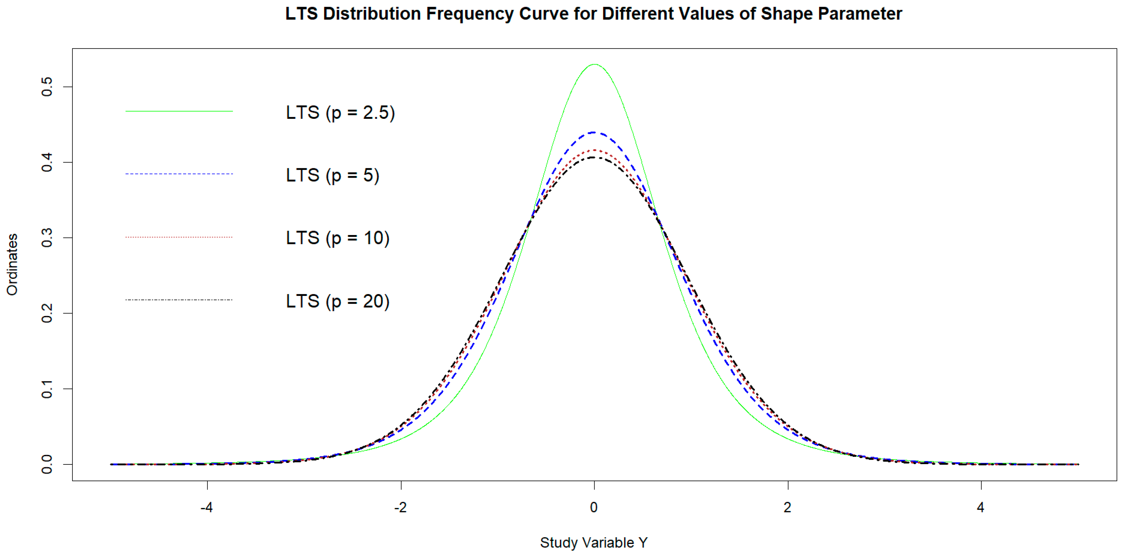
3.1. Long-Tailed Symmetric Family of Distribution

The long-tailed symmetric family of distribution is a general class of symmetric distribution that has a long tail on both ends while plotting a frequency curve. The process random variables $x_1,x_2,x_3,\dots ,x_n$ are assumed to be independently and identically distributed having a long-tailed symmetric distribution (LTS) with the probability density function (pdf) given as:

$$f\left(x\right):LTS\left(p,\theta ,\lambda \right)=\frac{1}{\lambda \sqrt{q}B\left(\frac{1}{2},p-\frac{1}{2}\right)}{\left\{1+\frac{{\left(x-\theta \right)}^2}{q{\lambda }^2}\right\}}^{-p},-\infty <x<\infty$$

(12)

where $p$ is the shape parameter and $q=2p-3$ for $p\ge 2$ with mean $E\left(x\right)=\theta$ and variance $\mathrm{var}\left(x\right)={\lambda }^2$, such as, $x_j\sim LTS\left(\theta ,{\lambda }^2\right)$. $B\left(\frac{1}{2},p-\frac{1}{2}\right)$ is the beta function which is equivalent to $B\left(\frac{1}{2},p-\frac{1}{2}\right)=\frac{\mathrm{\Gamma }\left(\frac{1}{2}\right)\mathrm{\Gamma }\left(p-\frac{1}{2}\right)}{\mathrm{\Gamma }\left(p\right)}$. Throughout this study, we assume that the value of $p$ is known; the plausible value of $p$ can be determined with the help of Q-Q plot in case $p$ is unknown. The kurtosis of (12) is ${\beta }_2=\frac{3q}{q-2}$ or ${\beta }_2=\frac{3}{\left(1-\frac{2}{q}\right)}$ and for $q\to \infty$, ${\beta }_2\to 0$, which means the LTS distribution reduces to normal distribution for $q\to \infty$ or equivalently $p\to \infty$. It is also worthwhile mentioning here that for $p$ = 1, (12) exhibits the same characteristics as that of the Cauchy distribution and for $p$ = 5, (12) becomes asymptotically symmetrical to logistic distribution with the first four moments in common. Huber [27] and Hampel et al. [28] identified that many real-life data sets can be mapped or approximated using the Student’s t-distribution. As a matter of fact, LTS distribution can be generated with the help of t-distribution and LTS is simply a scaled t-distribution with $\upsilon =2p-1$ degrees of freedom. Ahmed et al. [17] have pointed out that robust estimators which can counter outliers and deviations from the assumed distribution can be achieved via letting LTS distribution to epitomize the non-normal symmetrical phenomenon.

Figure 1 portrays the behavior of the LTS distribution at four different values of the shape parameter $p$. It can be seen that the shape of the LTS distribution is more heavily tailed than LTS ($p$ = 20). As discussed earlier, for $p$ = 20, LTS distribution reduces to a normal distribution as 20 is considered a very large value for the shape parameter.

3.2. Lloyd BLUE Estimator

Lloyd [29] proposed least square estimates of mean ($\theta$) and standard deviation ($\lambda$) by using order statistics. He showed the ordered estimate of $\overline{X}$ has a sampling variance which never exceeds that of the sample mean; it is equal to the sample mean provided the row totals of the variance–covariance matrix of the ordered observations have the same total. If the row totals are not the same, then the sampling variance of the ordered estimate of $\overline{X}$ has a strictly smaller variance than the sampling variance of $\overline{x}$.

By following his earlier work, let $x_1,x_2,\dots ,x_n$ be a simple random sample of size n from a long-tailed symmetrical family of distribution (12). Let $x_{\left(1\right)}\le x_{\left(2\right)}\le x_{\left(3\right)}\le \dots \le x_{\left(n\right)}$ be the order statistics of the said sample. Let $w_{\left(j\right)}=\frac{x_{\left(j\right)}-\theta }{\lambda }$ be the standardized variate of the order statistics $x_{\left(j\right)}$. Let the means, variances, and covariances of the order statistics from (12) be signified by $t_{\left(j\right)}$, ${\omega }_{jj}$, and ${\omega }_{ji}$, respectively. This can also be expressed symbolically as $E\left(w_{\left(j\right)}\right)=t_{\left(j\right)}$, $\mathrm{var}\left(w_{\left(j\right)}\right)={\omega }_{jj}$, $\mathrm{cov}\left(w_{\left(j\right)},w_{\left(i\right)}\right)={\omega }_{ji}$ for $j,i=1,2,3,\dots ,n$. The means, variances, and covariances of the order statistics $x_{\left(j\right)}$ of (12) are then be expressed as $E\left(x_{\left(j\right)}\right)=\theta +\lambda t_{\left(j\right)}$, $\mathrm{var}\left(x_{\left(j\right)}\right)={\lambda }^2{\omega }_{jj}$, $\mathrm{cov}\left(x_{\left(j\right)},x_{\left(i\right)}\right)={\lambda }^2{\omega }_{ji}$ for $j\le i$ and $j\ne i$. Moreover, $x^{\prime }=\left(x_{\left(1\right)},x_{\left(2\right)},\dots ,x_{\left(n\right)}\right)$, $t^{\prime }=\left(t_{\left(1\right)},t_{\left(2\right)},\dots ,t_{\left(n\right)}\right)$, $1^{\prime }=\left(1,1,\dots ,1\right)$, and $\Delta ={\omega }_{ji}$ or $j,i=1,2,3,\dots ,n$.

The best linear unbiased estimator (BLUE) of $\theta$ and $\lambda$ is given by Lloyd [29] for symmetrical distribution as,

$${\theta }^{\ast }=\frac{1^{\prime }{\Delta }^{-1}x}{1^{\prime }{\Delta }^{-1}1}\mathrm{or}{\theta }^{\ast }=\frac{{\displaystyle \sum _{j=1}^n{\displaystyle \sum _{i=1}^n{\nu }_{ji}}{x}_{\left(j\right)}}}{{\displaystyle \sum _{j=1}^n{\displaystyle \sum _{i=1}^n{\nu }_{ji}}}}={\displaystyle \sum _{j=1}^n{\gamma }_j{x}_{\left(j\right)}},$$

(13)

and

$${\lambda }^{\ast }=\frac{t^{\prime }{\Delta }^{-1}x}{t^{\prime }{\Delta }^{-1}t}\mathrm{or}{\lambda }^{\ast }=\frac{{\displaystyle \sum _{j=1}^n{\displaystyle \sum _{i=1}^n{\nu }_{ji}{t}_{\left(j\right)}{x}_{\left(j\right)}}}}{{\displaystyle \sum _{j=1}^n{\displaystyle \sum _{i=1}^n{\nu }_{ji}{t}_{\left(j\right)}{t}_{\left(i\right)}}}},$$

(14)

where $t^{\prime }$ is a row vector of elements $t_{\left(j\right)}$ for $j=1,2,3,\dots ,n$ and ${\gamma }_j={\displaystyle \sum _{i=1}^n{\nu }_{ji}}/{\displaystyle \sum _{j=1}^n{\displaystyle \sum _{i=1}^n{\nu }_{ji}}}$; ${\nu }_{ji}$ are the member elements of the inverse matrix $\Delta$. The variances in ${\theta }^{\ast }$ and ${\lambda }^{\ast }$ are given by

$$\mathrm{var}\left({\theta }^{\ast }\right)=\frac{{\lambda }^2}{1^{\prime }{\Delta }^{-1}1}\mathrm{or}\mathrm{var}\left({\theta }^{\ast }\right)=\frac{{\lambda }^2}{{\displaystyle \sum _{j=1}^n{\displaystyle \sum _{i=1}^n{\nu }_{ji}}}},$$

(15)

and

$$\mathrm{var}\left({\lambda }^{\ast }\right)=\frac{{\lambda }^2}{t^{\prime }{\Delta }^{-1}t}\mathrm{or}\mathrm{var}\left({\lambda }^{\ast }\right)=\frac{{\lambda }^2}{{\displaystyle \sum _{j=1}^n{\displaystyle \sum _{i=1}^n{\nu }_{ji}{t}_{\left(j\right)}{t}_{\left(i\right)}}}},$$

(16)

It is to be noted that the function ${\gamma }_j$ assigns higher weights to the central values and lower weights to the extreme values to nullify the effects of the outliers in the data. The value of $t_{\left(j\right)}$ may be determined by the relation,

$$F\left(w\right)={\displaystyle \underset{-\infty }{\overset{t_{\left(j\right)}}{\int }}f\left(w\right)dw}=\raisebox{1ex}{$j$}\!\left/ \!\raisebox{-1ex}{$\left(n+1\right)$}\right.,f\left(w\right)=\frac{1}{\sqrt{q}B\left(\frac{1}{2},p-\frac{1}{2}\right)}{\left\{1+\frac{w^2}{q}\right\}}^{-p},-\infty <w<\infty$$

(17)

The elements of $\Delta$, the variance covariance matrix of the order statistics of (12), may be determined from the equation given by

$${\omega }_{ji}\cong \frac{q_j\left(1-q_i\right)}{\left(n+2\right)f\left(v_j\right)f\left(v_i\right)},$$

(18)

where $q_j=j/\left(n+1\right)$, $q_i=i/\left(n+1\right)$, $F\left(v_j\right)=q_j$; where $v_j$ is a fractile of the reduced variable $u=\frac{x-\theta }{\lambda }$ with the cumulative density function $F\left(u\right)$ and $f\left(u\right)=F^{\prime }\left(u\right)$ is the density function of the LTS given in (12). The exact values of $t_{\left(j\right)}$ and $\Delta$ have been tabulated by Tiku and Kumra [30] and Vaughan [31]. Tiku and Kumra [30] had computed exact values of $t_{\left(j\right)}$ and $\Delta$ up to eight decimal places for $p=2(0.5)10$ and $n\le 20$.

Moreover, if subgroups of size n are used instead of individual observations and random variables are replaced with the means of the random variables of sizes “n” each, then the Lloyd’s BLUE estimator of mean ($\theta$) is given as:

$${\theta }^{\ast }=\frac{1^{\prime }{\Delta }^{-1}{\mu }^{\ast }}{1^{\prime }{\Delta }^{-1}1}\mathrm{or}{\theta }^{\ast }=\frac{{\displaystyle \sum _{j=1}^n{\displaystyle \sum _{i=1}^n{\nu }_{ji}}{\mu }_{\left(j\right)}^{\ast }}}{{\displaystyle \sum _{j=1}^n{\displaystyle \sum _{i=1}^n{\nu }_{ji}}}}={\displaystyle \sum _{j=1}^n{\gamma }_j{\mu }_{\left(j\right)}^{\ast }},$$

(19)

Also, the variance of the ${\theta }^{\ast }$ is given as:

$$\mathrm{var}\left({\theta }^{\ast }\right)=\frac{\raisebox{1ex}{${\lambda }^2$}\!\left/ \!\raisebox{-1ex}{$n$}\right.}{1^{\prime }{\Delta }^{-1}1}\mathrm{or}\mathrm{var}\left({\theta }^{\ast }\right)=\frac{\raisebox{1ex}{${\lambda }^2$}\!\left/ \!\raisebox{-1ex}{$n$}\right.}{{\displaystyle \sum _{j=1}^n{\displaystyle \sum _{i=1}^n{\nu }_{ji}}}},$$

(20)

where ${\mu }^{\ast }$ is the vector of means of size n.

3.3. Proposed Scheme of Mixed Exponentially Weighted Moving Average—Cumulative Sum Control Chart

In this subsection, we suggest a concoction of the classic CUSUM and EWMA schemes via mingling the features of their design structures. The proposed mixed exponentially weighted moving average—cumulative sum (M_xEC) control chart is based on two statistics called $P{S}_j^{+}$ and $P{S}_j^{-}$, which are delimited as:

$$\left.\begin{array}{l}P{S}_j^{+}=\max \left[0,\left(R_j-{\theta }_0\right)-K_{R_j}+P{S}_{j-1}^{+}\right]\\ P{S}_j^{-}=\max \left[0,-\left(R_j-{\theta }_0\right)-K_{R_j}+P{S}_{j-1}^{-}\right]\end{array}\right\},$$

(21)

where $K_{R_j}$ is the time-varying reference value or the slack value for the suggested charting structure, and the quantities $P{S}_j^{+}$ and $P{S}_j^{-}$ are recognized as the upper and lower CUSUM statistics, respectively, and are based on the EWMA statistic $R_j$ which is defined as:

$$R_j={\phi }_r{\theta }^{\ast }+\left(1-{\phi }_r\right)R_{j-1},$$

(22)

where ${\phi }_r$ in (22) is the smoothing constant such that $0<{\phi }_r\le 1$ and ${\theta }^{\ast }$ is the best linear unbiased estimator of mean given in (19). Furthermore, the initial value of the EWMA statistic $R_j$ is set equal to the target mean value, such as, $R_0={\theta }_0$. The mean and variance of the EWMA statistic $R_j$ is given as:

$$Mean\left(R_j\right)={\theta }_0\mathrm{and}Var\left(R_j\right)=\mathrm{var}\left({\theta }^{\ast }\right)\left[\frac{{\phi }_r}{2-{\phi }_r}\left(1-{\left(1-{\phi }_r\right)}^{2j}\right)\right],$$

(23)

In the above Equations (21) and (22), we are considering the case of subgroups of size n, where $n\ge 2$, for individual observations use n = 1. The two statistics $P{S}_j^{+}$ and $P{S}_j^{-}$ are plotted against the control limit, say $H_{R_j}$. The process remains in-control state till the values of $P{S}_j^{+}$ and $P{S}_j^{-}$ are plotted inside the control limit $H_{R_j}$, otherwise the process is a victim of out-of-control state. Interestingly, if the statistic $P{S}_j^{+}$ is plotted above the control limit $H_{R_j}$, the process mean is increasing and said to be shifted above the target mean value, and if the statistic $P{S}_j^{-}$ is plotted above the control limit $H_{R_j}$, the process mean is showing a negative shift and said to be shifted below the target mean value. The control limit $H_{R_j}$ is selected according to a prefixed value of ARL₀. There exists a direct proportion between the prefixed value of ARL₀ and the control limit $H_{R_j}$. For a large value of prefixed ARL₀, a large value of control limit $H_{R_j}$ is required and vice versa. The three key parameters of the proposed M_xEC control chart are ${\phi }_r$, $K_{R_j}$, and $H_{R_j}$. The quantities $K_{R_j}$ and $H_{R_j}$ can be expressed by using the formulas given as:

$$\left.\begin{array}{l}{K}_{R_j}=k_R^{\ast }\sqrt{\mathrm{var}\left(R_j\right)}=k_R^{\ast }\sqrt{\mathrm{var}\left({\theta }^{\ast }\right)\left[\frac{{\phi }_r}{2-{\phi }_r}\left(1-{\left(1-{\phi }_r\right)}^{2j}\right)\right]}\\ H_{R_j}=h_R^{\ast }\sqrt{\mathrm{var}\left(R_j\right)}=h_R^{\ast }\sqrt{\mathrm{var}\left({\theta }^{\ast }\right)\left[\frac{{\phi }_r}{2-{\phi }_r}\left(1-{\left(1-{\phi }_r\right)}^{2j}\right)\right]}\end{array}\right\},$$

(24)

where $k_R^{\ast }$ and $h_R^{\ast }$ are constant values normally used to fix the predefined false alarm rate and to obtain the prefixed value of ARL₀ just like the constants $k_E^{\ast }$ and $h_E^{\ast }$ in (10) and (11). The expression for the $\mathrm{var}\left({\theta }^{\ast }\right)$ is given in (20). It is worthwhile mentioning here that $\theta$ and ${\lambda }^2$ are the population mean and variance, respectively. If these two population parameters are not known, then these two unknown parameters can be estimated by using the preliminary samples. Moreover, the random variable $x_j$ is following a long-tailed symmetric family of distribution given in (12). The constants $k_R^{\ast }$ and $h_R^{\ast }$ in (24) are just like the constants k and h in the traditional CUSUM control chart. We can choose the value of $h_R^{\ast }$ from the tables (provided later in the next section) for a prefixed ARL₀ at our desired level. As a matter of fact, a good working practice is to choose $k_R^{\ast }$ equal to exactly half of the shift size (in units of the standard deviation of $R_j$). Therefore, we choose $k_R^{\ast }=0.5$ due to the fact that it makes the CUSUM structure more subtle to small or moderate shifts of magnitude less than or equal to 1.5 times the standard deviations (Montgomery [2]).

4. Performance Measure of Proposed and Conventional Control Charts

There are several techniques available to gauge the performance of the control charts. By exploring the literature, we find different techniques that have been used by researchers to compare and evaluate the performance of the control charts, which includes Markov chains, integral equations, extra quadratic loss, performance comparison index study, relative average run lengths, Monte Carlo simulations, and various types of approximations. In this study, we have used the Monte Carlo algorithm to evaluate the performance of the control charts by computing average run lengths (ARLs). R programming language has been used to develop the programmes to calculate the run lengths. In order to obtain the desired values of ARL₀ (the in-control average run length value), the algorithm is repeated 50,000 times to compute the average of those 50,000 run lengths. A comprehensive study on the performance of the ARLs of the proposed mixed EWMA-CUSUM (M_xEC) control chart to efficiently monitor the process mean of a non-normal but symmetrical distribution is given in

Table 13. Run length profile of the proposed mixed EWMA-CUSUM (M_xEC) control chart scheme under $LTS(2.5,0,1)$ at ARL₀ = 168.

${\mathit{\phi }}_{\mathit{r}}$ $=0.5,{\mathit{k}}_{\mathit{R}}^{\ast }$ $=0.5,{\mathit{h}}_{\mathit{R}}^{\ast }$ = 5.61, n = 10
$\mathit{\delta }$	ARL	SDRL	P25	P50	P75	P90
0	167.50	160.97	52	117	230	380
0.25	11.61	6.24	7	10	14	20
0.5	5.12	1.54	4	5	6	7
0.75	3.53	0.79	3	3	4	5
1	2.79	0.56	2	3	3	3
1.5	2.05	0.23	2	2	2	2
2	1.86	0.34	2	2	2	2

,

Table 14. Run length profile of the proposed mixed EWMA-CUSUM (M_xEC) control chart scheme under $LTS(2.5,0,1)$ at ARL₀ = 400.

${\mathit{\phi }}_{\mathit{r}}$ $=0.5,{\mathit{k}}_{\mathit{R}}^{\ast }$ $=0.5,{\mathit{h}}_{\mathit{R}}^{\ast }$ = 7.32, n = 10
$\mathit{\delta }$	ARL	SDRL	P25	P50	P75	P90
0	402.67	394.23	122.75	280	553	902
0.25	14.55	14.55	9	13	18	24.1
0.5	6.15	6.15	5	6	7	8
0.75	4.19	4.19	4	4	5	5
1	3.30	3.30	3	3	4	4
1.5	2.37	2.37	2	2	3	3
2	2	2	2	2	2	2

,

Table 15. Run length profile of the proposed mixed EWMA-CUSUM (M_xEC) control chart scheme under $LTS(2.5,0,1)$ at ARL₀ = 500.

${\mathit{\phi }}_{\mathit{r}}$ $=0.5,{\mathit{k}}_{\mathit{R}}^{\ast }$ $=0.5,{\mathit{h}}_{\mathit{R}}^{\ast }$ = 7.77, n = 10
$\mathit{\delta }$	ARL	SDRL	P25	P50	P75	P90
0	498.81	484.28	155	348	687	1120.1
0.25	15.15	7.54	10	13	19	25
0.5	6.43	1.78	5	6	7	9
0.75	4.36	0.88	4	4	5	5
1	3.43	0.59	3	3	4	4
1.5	2.51	0.50	2	3	3	3
2	2.02	0.13	2	2	2	2

and

Table 16. ARL values for the proposed EWMA-CUSUM (M_xEC) control chart scheme under $LTS(2.5,0,1)$ with n = 10, $k_R^{\ast }$ = 0.5.

$\mathit{\delta }$	${\mathit{\phi }}_{\mathit{r}}$ = 0.1 ${\mathit{h}}_{\mathit{R}}^{\ast }$ = 14.49	${\mathit{\phi }}_{\mathit{r}}$ = 0.25 ${\mathit{h}}_{\mathit{R}}^{\ast }$ = 9.17	${\mathit{\phi }}_{\mathit{r}}$ = 0.75 ${\mathit{h}}_{\mathit{R}}^{\ast }$ = 3.87	${\mathit{\phi }}_{\mathit{r}}$ = 0.1 ${\mathit{h}}_{\mathit{R}}^{\ast }$ = 23.33	${\mathit{\phi }}_{\mathit{r}}$ = 0.25 ${\mathit{h}}_{\mathit{R}}^{\ast }$ = 12.83	${\mathit{\phi }}_{\mathit{r}}$ = 0.75 ${\mathit{h}}_{\mathit{R}}^{\ast }$ = 4.85	${\mathit{\phi }}_{\mathit{r}}$ = 0.1 ${\mathit{h}}_{\mathit{R}}^{\ast }$ = 25.92	${\mathit{\phi }}_{\mathit{r}}$ = 0.25 ${\mathit{h}}_{\mathit{R}}^{\ast }$ = 14.12	${\mathit{\phi }}_{\mathit{r}}$ = 0.75 ${\mathit{h}}_{\mathit{R}}^{\ast }$ = 5.10
0	168.98	168.40	167.80	401.15	399.88	401.08	499.96	500.82	500.41
0.25	15.18	12.70	11.56	20.15	15.81	14.34	21.42	16.92	15.31
0.5	8.59	6.49	4.52	11.46	8.02	5.38	12.20	8.55	5.59
0.75	6.32	4.71	2.93	8.49	5.77	3.44	9.04	6.13	3.55
1	5.13	3.77	2.25	6.91	4.66	2.61	7.39	4.96	2.70
1.5	3.88	2.88	1.73	5.19	3.45	1.98	5.56	3.74	2.01
2	3.06	2.16	1.16	4.18	2.96	1.58	4.57	3.02	1.70

for some specific values of $\delta$, ${\phi }_r$, and $h_R^{\ast }$. The prefixed values of the in-control ARL are set at 168, 400, and 500, which are the frequently used choices available in the literature. On the same guidelines, one may achieve other values of ARL₀ for different choices of parameters.

In addition to the ARL values presented in Table 13, Table 14, Table 15 and Table 16, relative standard errors for these results have also been calculated and it was observed that they are all below 1.1%. By ensuring that the relative standard errors are within an acceptable range and validating our simulation algorithm against established results, we can have confidence in the reliability and validity of the presented ARL values and their implications for the performance of the control chart schemes.

Some of the key takeaways about our proposed EWMA-CUSUM control chart scheme under $LTS\left(p=2.5,\theta =0,\lambda =1\right)$ for monitoring the process mean are:

• For true comparison purposes, the time varying reference value $k_R^{\ast }$ has been kept fixed at 0.5 (Table 13, Table 14 and Table 15).
• With the increase in the shift constant ($\delta$), the values of ARL, SDRL, and percentiles decreases (Table 13, Table 14 and Table 15).
• The value of ARL increases with the increase in control limit ($h_R^{\ast }$) (see Table 16).
• When the smoothing constant (${\phi }_r$) increases, then the control limit ($h_R^{\ast }$) decreases, to achieve the fixed ARL₀ (Table 16).
• The value of ARL₁ decreases with the increase in smoothing constant (${\phi }_r$) (Table 16).
• The value of ARL₁ goes down with the decrease in control limit ($h_R^{\ast }$) (see Table 16).
• The ARL values represent the average number of observations or samples required for the control chart to signal an out-of-control condition. The control chart scheme triggers an alarm within a few samples, as evidenced by the small ARL values, particularly for large shift sizes. The control chart scheme exhibits high sensitivity to small shifts in the process mean, as indicated by the ARL values of 15.15 and 6.43 for shift sizes of 0.25 and 0.5, respectively. This suggests that even relatively small deviations from the mean will be promptly detected by the control chart (Table 15).
• The SDRL values provide an indication of the variability or dispersion in the run lengths. Smaller SDRL values suggest more consistent performance and less variability in detecting shifts (Table 13, Table 14 and Table 15).
• The percentile values (P25, P50, P75, P90) indicate that most shifts are detected within a reasonable number of samples, with higher percentiles representing longer run lengths for extreme cases (Table 13, Table 14 and Table 15).
• The control chart scheme achieves very low ARL values of 4.19 and 3.30 for shift sizes of 0.75 and 1, respectively, for a fixed ARL₀ values of 400 (Table 14). This indicates that moderate shifts in the process mean can be detected efficiently with a relatively small number of samples.
• The control chart scheme exhibits quick detection of shifts, as indicated by the low percentile values (P25, P50, P75, P90) for all shift sizes. This implies that the majority of shifts are detected within a relatively short period (Table 13, Table 14 and Table 15).

These insights highlight the sensitivity, efficiency, stability, and early detection capabilities of the proposed EWMA-CUSUM control chart scheme under $LTS\left(2.5,0,1\right)$ for various shift sizes, reaffirming its effectiveness in detecting shifts in the process mean.

5. Comparisons

This section provides a comprehensive comparison between the proposed mixed EWMA-CUSUM scheme and several existing representative control charts, including classic CUSUM, classic EWMA, FIR-CUSUM, FIR-EWMA, classic Shewhart, adaptive CUSUM with EWMA-based shift estimator, adaptive EWMA, weighted CUSUM, mixed EWMA-CUSUM, and run rules-based CUSUM and EWMA. The performance of these control charts is evaluated based on their ARL values. By examining all the available tables, we can gain insights into how the proposed mixed EWMA-CUSUM scheme performs in relation to the other control charts discussed in the literature.

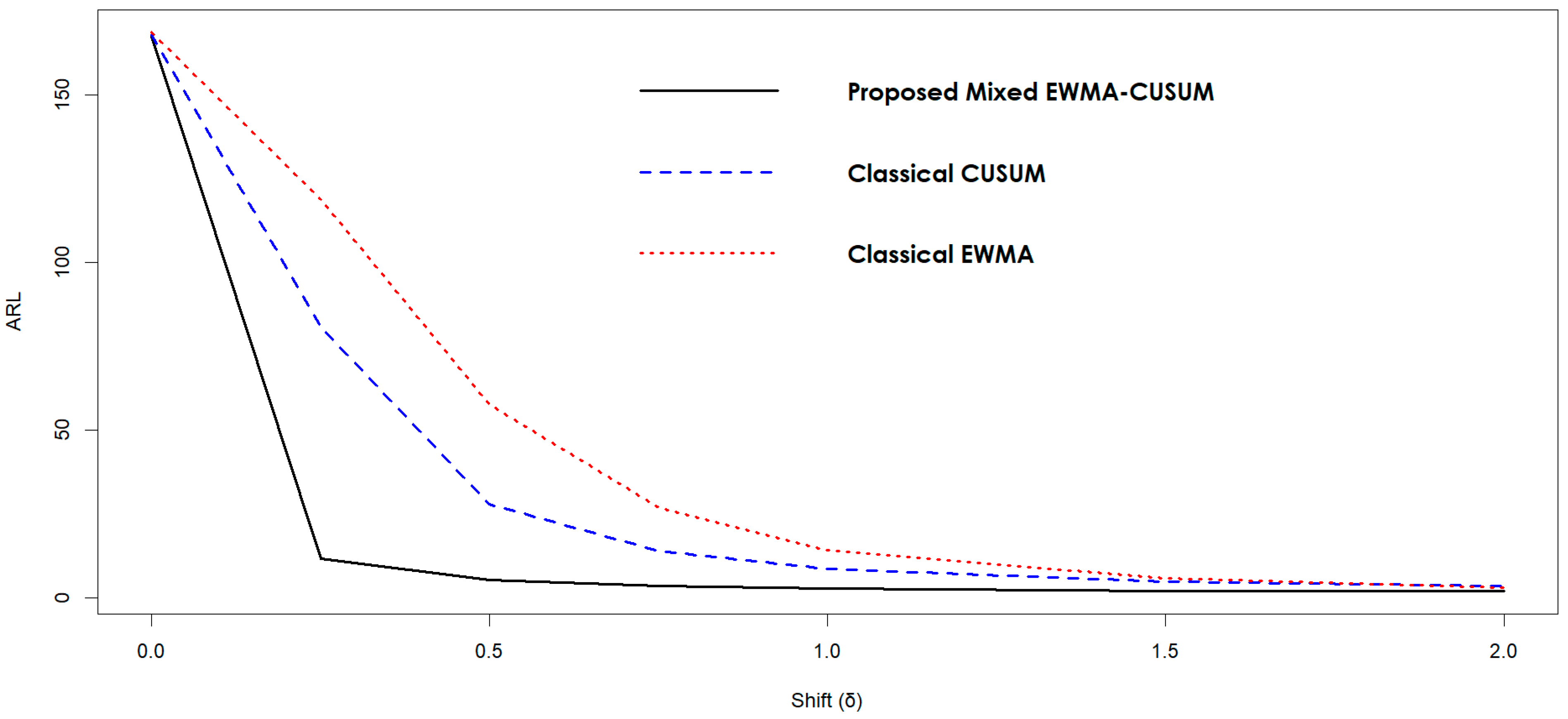
5.1. Proposed Mixed EWMA-CUSUM (MxEC) vs. Classical CUSUM

The different values of ARL for the classic CUSUM control chart scheme proposed by Page [3] are presented in Table 4. Meanwhile, Table 1, Table 2 and Table 3 provide insights about complete run length profile for different ARL₀ values equivalent to 168, 400, and 500, respectively, under $LTS(2.5,0,1)$. The proposed control scheme presented in Table 13, Table 14, Table 15 and Table 16 has outclassed the CUSUM control chart in terms of performance and efficiency in detecting small to moderate shifts in the process mean for all values of ${\phi }_r$. Especially, the performance of proposed scheme is outstanding in the case of $\delta \le 1$, when compared with the classic CUSUM scheme.

5.2. Proposed Mixed EWMA-CUSUM (MxEC) vs. FIR-CUSUM

The FIR-CUSUM introduced by Lucas and Crosier [7] offers a head start to the CUSUM statistic. The head start is represented with S₀ and the ARLs of the CUSUM with FIR features are provided in the subsequent tables (

Table 17. ARL values for the FIR CUSUM scheme with n = 10 and $K$ = 0.5 at ARL₀ = 168.

$\mathit{\delta }$	0	0.25	0.5	0.75	1	1.5	2
$H$ = 4, S0 = 1	162.56	71.16	24.38	11.74	7.16	3.87	2.71
$H$ = 4, S0 = 2	148.93	62.77	20.21	8.99	5.32	2.91	2.04

,

Table 18. Run length profile of FIR-CUSUM control chart scheme under $LTS\left(2.5,0,1\right)$ with n = 10 at ARL₀ = 168.

	$\mathit{K}=0.5,$ $\mathit{H}$ = 4.14, S0 = 1						$\mathit{K}=0.5,$ $\mathit{H}$ = 4.21, S0 = 2
$\mathit{\delta }$	ARL	SDRL	P25	P50	P75	P90	ARL	SDRL	P25	P50	P75	P90
0	167.08	164.23	50	118	231	375	166.97	178.26	39	111	235	403
0.25	78.57	77.70	23	54	109	181	73.24	78.13	16.75	49	104	173
0.5	26.73	23.84	10	20	36	57	22.67	23.06	6	15	32	53
0.75	12.08	8.99	6	10	16	24	9.95	8.89	4	7	13	22
1	7.27	4.59	4	6	9	13	5.65	4.16	3	4	7	11
1.5	3.95	1.85	3	4	5	6	3.08	1.67	2	3	4	5
2	2.79	1.06	2	3	3	4	2.16	0.94	2	2	3	3

,

Table 19. Run length profile of FIR-CUSUM control chart scheme under $LTS\left(2.5,0,1\right)$ with n = 10 at ARL₀ = 400.

	$\mathit{K}=0.5,$ $\mathit{H}$ = 5.08, S0 = 1						$\mathit{K}=0.5,$ $\mathit{H}$ = 5.09, S0 = 2
$\mathit{\delta }$	ARL	SDRL	P25	P50	P75	P90	ARL	SDRL	P25	P50	P75	P90
0	400.42	401.65	115	277	554	915	400.09	406.43	109	278	555	937
0.25	143.07	142.17	43	99	196	321	133.79	136.15	36	91	185	318
0.5	37.69	32.85	14	28	50	81	33.56	31.75	11	24	46	75
0.75	15.79	11.43	8	12	20	31	13.18	10.59	6	10	17	28
1	9.31	5.40	5.75	8	12	16	7.57	5.02	4	6	10	14
1.5	4.90	2.07	3	4	6	8	3.93	1.89	3	4	5	6
2	3.42	1.18	3	3	4	5	2.77	1.06	2	3	3	4

and

Table 20. Run length profile of FIR-CUSUM control chart scheme under $LTS\left(2.5,0,1\right)$ with n = 10 at ARL₀ = 500.

	$\mathit{K}=0.5,$ $\mathit{H}$ = 5.34, S0 = 1						$\mathit{K}=0.5,$ $\mathit{H}$ = 5.35, S0 = 2
$\mathit{\delta }$	ARL	SDRL	P25	P50	P75	P90	ARL	SDRL	P25	P50	P75	P90
0	501.05	498.24	145	347	701	1143.1	500.73	501.65	140	345	701	1164.1
0.25	163.25	160.12	51	114	225	367	157.81	162.21	42	108	219	373
0.5	40.79	34.65	16	31	55	85.1	37.40	35.93	12	26	51	85
0.75	16.72	11.66	8	14	22	32	14.15	11.38	6	11	18	29
1	9.75	5.59	6	8	12	17	7.92	5.06	4	7	10	15
1.5	5.21	2.17	4	5	6	8	4.20	1.95	3	4	5	7
2	3.61	1.24	3	3	4	5	2.94	1.10	2	3	3	4

). Table 17 indicates the abatement in the ARL₀ values by including FIR in CUSUM chart, and notably, ARL₀ becomes very small for large values of S₀ (S₀ = 2, ARL₀ = 148.93).

Table 18, Table 19 and Table 20 refer to the complete run length profiles of FIR-CUSUM for two choices of head start value S₀ = 1, 2. By comparing these tables with the proposed control chart (Table 13, Table 14 and Table 15), it is evident that our proposed control chart scheme has beaten the FIR-CUSUM scheme by a big margin in terms of performance and quick detection of change in the process mean. For small shift sizes, our proposed scheme performs even better and detects the change in much smaller samples than its counterpart.

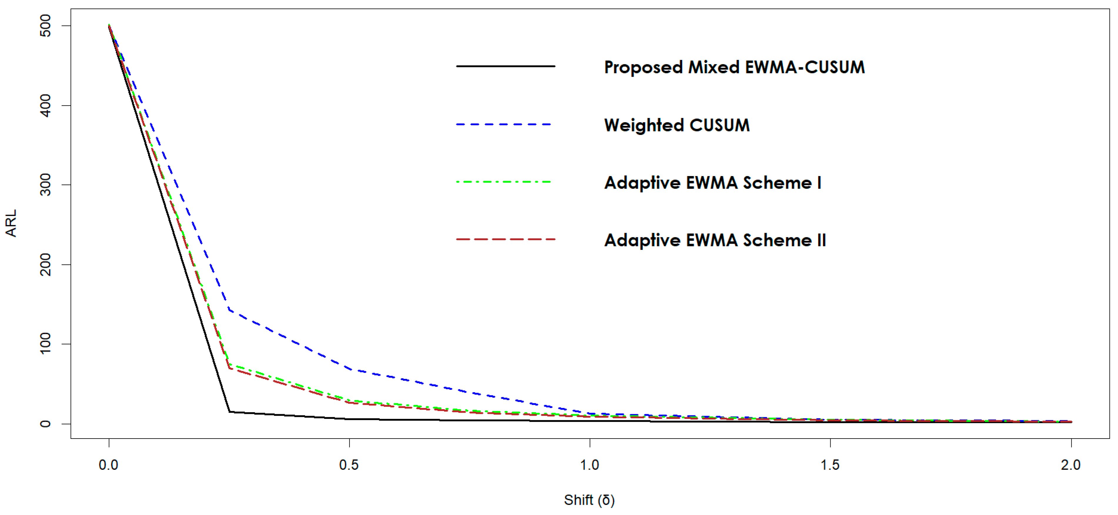
5.3. Proposed Mixed EWMA-CUSUM (MxEC) vs. Weighted CUSUM

Yashchin [32] came up with an idea of a weighted CUSUM in which he assigned weights (represented with ϒ) to the past observations in the CUSUM statistic. By comparing

Table 21. ARL values for the symmetric two-sided weighted CUCUM scheme under $LTS\left(2.5,0,1\right)$ with n = 10 at ARL₀ = 500.

$\mathit{K}$= 0.5		$\mathit{\delta }$
Υ	$\mathit{H}$	0.5	1	1.5	2
0.7	3.16	85.94	15.78	6.05	3.50
0.8	3.46	69.37	13.27	5.63	3.49
0.9	3.97	53.93	11.29	5.49	3.58
1.0	5.09	38.98	10.42	5.72	4.00

with the corresponding tables of proposed control scheme (see Table 15 and Table 16), it is evident that our proposed scheme has an advantage over the weighted CUSUM scheme by a long margin. Our proposed chart clearly outperforms the weighted CUSUM chart when small to moderate shifts are to be detected ($\delta \le 1$), and for large shift sizes the gap between the ARL values fills up.

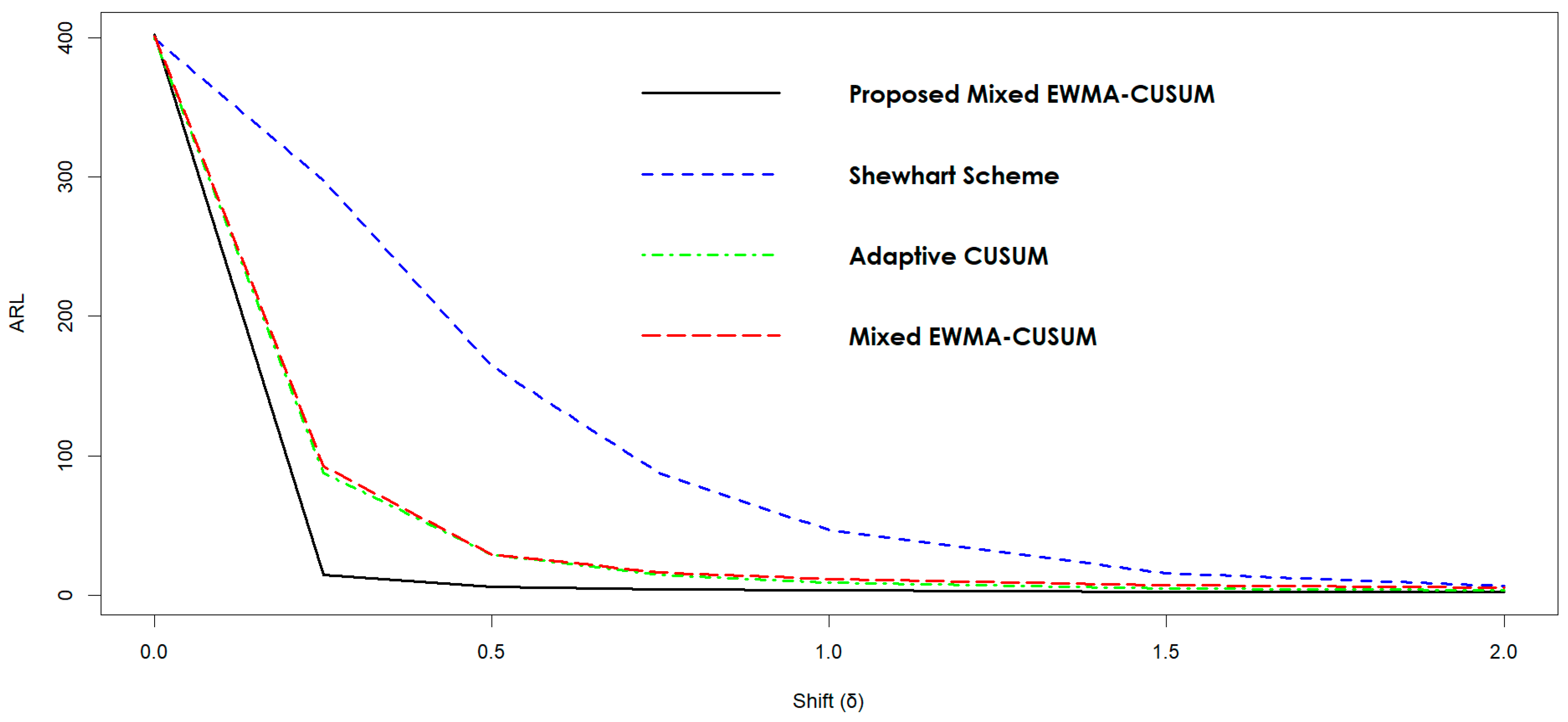
5.4. Proposed Mixed EWMA-CUSUM (MxEC) vs. Adaptive CUSUM

Jiang et al. [33] introduced a novel approach that combines adaptive CUSUM with an EWMA-based shift estimator. Their method involves dynamically updating the reference value of the CUSUM chart using the EWMA estimator and a suitable weighting function. The ARL values for the adaptive CUSUM, which are presented in

Table 22. ARL values for the adaptive CUSUM under $LTS\left(2.5,0,1\right)$ with ${\delta }_{\min }^{+}$, n = 10, $\lambda$ = 0.3 at ARL₀ = 400.

$\mathit{\delta }$	$\mathit{\phi }$ = 1.5 $\mathit{h}$ = 5.07	$\mathit{\phi }$ = 2 $\mathit{h}$ = 4.79	$\mathit{\phi }$ = 3 $\mathit{h}$ = 4.425	$\mathit{\phi }$ = 4 $\mathit{h}$ = 4.355	$\mathit{\phi }=$ $\mathit{\infty }$ $\mathit{h}$ = 4.345
0	398.32	401.93	400.36	398.97	401.03
0.25	92.73	91.64	87.41	85.92	85.82
0.5	30.24	30.17	28.88	28.54	28.37
0.75	14.68	14.54	14.23	13.79	13.43
1	9.13	8.97	8.78	8.54	8.21
1.5	4.92	4.78	4.87	4.81	4.78
2	3.25	3.23	3.32	3.28	3.26

along with the parameters of the chart, namely ${\delta }_{\min }^{+}$, $\lambda$, $\phi$, and $h$, are also specified. Upon comparing the performance of the proposed approach, it is evident that it outperforms the adaptive CUSUM when dealing with small and moderate values of $\delta$. However, for large values of $\delta$, both the proposed approach and the adaptive CUSUM exhibit almost similar ARL performance, as depicted in the tables.

5.5. Proposed Mixed EWMA-CUSUM (MxEC) vs. Run Rules-Based CUSUM

Action limit (AL) and warning limit (WL) are key parameters in the CUSUM chart used for monitoring processes. The AL represents a threshold level for the CUSUM chart statistic, and if the statistic exceeds this limit, it indicates that the process is out of control. The AL value is typically greater than the critical limit ($H$) used for determining out-of-control situations with a fixed average run length (ARL₀).

On the other hand, the WL is a level for the CUSUM chart statistics, where consecutive points show a pattern that suggests an out-of-control situation, but without crossing the AL. The WL value is usually smaller than the critical level ($H$) for a fixed ARL₀. Based on these definitions, Riaz et al. [9] proposed two schemes for the CUSUM chart:

• Scheme I: A process is considered out of control if any of the following conditions are met:
  • A single data point of the positive CUSUM (S+) falls outside the AL.
  • A single data point of the negative CUSUM (S-) falls outside the AL.
  • Two consecutive data points of S+ fall between the WL and the AL.
  • Two consecutive data points of S- fall between the WL and the AL.
• Scheme II: A process is deemed out of control if any of the following conditions are met:
  • A single data point of S+ falls outside the AL.
  • A single data point of S- falls outside the AL.
  • Two out of three consecutive data points of S+ fall between the WL and the AL.
  • Two out of three consecutive data points of S- fall between the WL and the AL.

The ARLs for the two run rules-based CUSUMs are given in

Table 23. ARL values for the run rules-based CUCUM under $LTS\left(2.5,0,1\right)$ with n = 10 at ARL₀ = 168.

Scheme I
Limits		$\mathit{\delta }$
WL	AL	0.25	0.5	0.75	1	1.5	2
3.42	4.8	71.97	25.65	13.54	8.66	5.17	3.68
3.44	4.6	72.38	25.72	13.5	8.57	5.11	3.61
3.48	4.4	71.94	25.62	13.49	8.52	4.94	3.53
3.53	4.2	71.48	25.34	13.33	8.41	4.83	3.43
Scheme II
3.5	4.44	71.49	25.38	13.40	8.46	4.94	3.54
3.6	4.19	72.94	25.37	13.35	8.38	4.83	3.44
3.7	4.08	73.11	25.37	13.31	8.34	4.78	3.38
3.8	4.03	73.59	25.41	13.28	8.32	4.75	3.35

and

Table 24. ARL values for the run rules-based CUCUM under $LTS\left(2.5,0,1\right)$ with n = 10 at ARL₀ = 500.

Scheme I
Limits		$\mathit{\delta }$
WL	AL	0.25	0.5	0.75	1	1.5	2
4.8	5.12	141.12	38.60	17.39	10.52	5.91	4.06
4.7	5.2	150.38	38.62	17.63	10.61	5.90	4.15
4.6	5.39	145.21	38.21	17.47	10.56	6.01	4.24
4.5	∞	146.74	38.47	17.73	10.83	6.32	4.71
Scheme II
4.8	5.11	139.72	38.87	17.48	10.53	5.83	4.11
4.7	5.2	142.17	37.98	17.28	10.59	5.87	4.10
4.6	5.5	145.79	38.34	17.39	10.76	6.08	4.28
4.55	∞	149.13	39.93	17.59	10.98	6.47	4.88

. The comparison of the proposed control chart scheme with these tables indicates that the proposed scheme has the ability to perform better than the run rules-based CUSUM for any combination of parameter choices.

5.6. Proposed Mixed EWMA-CUSUM (MxEC) vs. Shewhart Scheme

Shewhart’s [1] control chart scheme is a very popular technique to monitor shifts in the process parameter. The ARL values for the Shewhart control chart scheme for a subgroup of size 10 is given in

Table 25. ARL values of Shewhart Mean ($\overline{X}$) control chart under $LTS\left(2.5,0,1\right)$ with n = 10.

$\mathit{\delta }$	0	0.25	0.5	0.75	1	1.5	2
ARL at L = 2.75	168.55	131.38	77.65	43.58	25.05	9.38	4.40
ARL at L = 3.024	399.74	297.59	164.39	87	46.63	15.69	6.50
ARL at L = 3.09	501.13	370.83	201.60	101.63	55.54	17.98	7.18

. Clearly, our proposed scheme offers superior ability over the Shewhart control chart scheme.

5.7. Proposed Mixed EWMA-CUSUM (MxEC) vs. Classical Time-Varying EWMA

The ARL values of the time-varying classic EWMA control chart by Roberts [4] are given in Table 5, Table 6, Table 7 and Table 8. For different choices of $\phi$ and a fixed value of $k_R^{\ast }$, the proposed scheme is compared with a classic EWMA scheme. It has been observed that the proposed scheme has a better performance in terms of ARL₁ for different choices of $\phi$. In particular, for smaller shift sizes ($\delta \le 1$), the proposed scheme quickly detects the change in the process mean as compared to the classic EWMA scheme.

5.8. Proposed Mixed EWMA-CUSUM (MxEC) vs. FIR-EWMA

Steiner [8] introduced the concept of FIR EWMA, which shares similarities with FIR CUSUM by providing an advantageous starting point for the EWMA statistic. Upon comparing the suggested approach to FIR-EWMA, we discovered that the suggested scheme outperforms FIR-EWMA when dealing with minor and moderate shifts ($\delta \le 1$). However, for substantial shifts, FIR-EWMA appears to be on a par with the proposed chart. FIR-EWMA scheme is presented in

Table 26. ARL values for the FIR EWMA scheme under $LTS\left(2.5,0,1\right)$ with n = 10 at ARL₀ = 500.

$\mathit{\delta }$	% Head Start	$\mathit{\phi }$ = 0.1 $\mathit{W}$ = 2.824	$\mathit{\phi }$ = 0.25 $\mathit{W}$ = 3	$\mathit{\phi }$ = 0.5 $\mathit{W}$ = 3.072	$\mathit{\phi }$ = 0.75 $\mathit{W}$ = 3.088
0	25	489	494	496	499.15
	50	471	486	488	496.54
0.5	25	29.45	47.34	88.13	141.05
	50	26.39	44.07	86.89	139.67
1	25	8.97	10.38	17.27	30.48
	50	6.88	8.97	16.38	29.83
2	25	3.64	3.23	3.74	4.47
	50	2.91	2.56	2.98	4.26

.

5.9. Proposed Mixed EWMA-CUSUM (MxEC) vs. Adaptive EWMA

Zaman et al. [34] proposed two adaptive EWMA schemes based on Huber’s function and Tukey’s bisquare function of prediction errors, respectively.

Table 27. Run length profile of the adaptive EWMA scheme I and II under $LTS(2.5,0,1)$ with n = 10 at ARL₀ = 500.

$\mathit{K}$ = 0.5, $\mathit{\phi }$ = 0.1, Υ = 4.15, $\mathit{W}$ = 4.865 (Scheme I)						$\mathit{K}$ = 0.2, $\mathit{\phi }$ = 0.05, Υ = 31.12, $\mathit{W}$ = 8.95 (Scheme II)
$\mathit{\delta }$	ARL	SDRL	P25	P50	P75	P90	ARL	SDRL	P25	P50	P75	P90
0	501.29	498.75	139	348	695	1168	500.01	497.62	135	344	689	1154
0.25	75.38	73.18	26	55	112	178	70.17	62.59	26	53	109	172
0.5	29.47	26.94	11	22	37	49	26.23	22.36	12	21	35	48
0.75	16.68	13.67	6	10	16	22	14.17	10.82	6	11	14	21
1	10.25	8.51	3	6	11	15	8.98	4.12	4	7	9	12
1.5	5.25	3.79	2	3	5	7	4.82	1.98	2	4	5	7
2	3.26	1.18	1	2	3	4	2.99	1.09	1	2	3	4

refers to the run length profile of adaptive EWMA for scheme I and II. Unlike traditional EWMA charts with fixed control limits, the adaptive EWMA method incorporates an adaptive factor that adjusts the smoothing constant of the EWMA statistic based on the historical data. This adaptive factor allows the control limits to adapt and change in response to shifts in process behavior, ensuring that the chart remains sensitive to detecting changes in the process mean.

Upon conducting a comparative analysis between our proposed scheme and the adaptive EWMA Schemes I and II, we observed that our proposed scheme exhibits superior performance in relation to the ARL₁ values.

5.10. Proposed Mixed EWMA-CUSUM (MxEC) vs. Runs Rules-Based EWMA

Abbas et al. [10] introduced the concept of integrating run rules schemes into the structure of EWMA charts. They provided ARLs for two run rules-based EWMA schemes in

Table 28. ARL values of the run rules-based EWMA under $LTS(2.5,0,1)$ with n = 10 at ARL₀ = 500.

Scheme I					Scheme II
$\mathit{\delta }$	${\mathit{\phi }}_{\mathit{s}}$ = 0.1 ${\mathit{W}}_{\mathit{s}}$ = 2.556	${\mathit{\phi }}_{\mathit{s}}$ = 0.25 ${\mathit{W}}_{\mathit{s}}$ = 2.554	${\mathit{\phi }}_{\mathit{s}}$ = 0.5 ${\mathit{W}}_{\mathit{s}}$ = 2.36	${\mathit{\phi }}_{\mathit{s}}$ = 0.75 ${\mathit{W}}_{\mathit{s}}$ = 2.115	${\mathit{\phi }}_{\mathit{s}}$ = 0.1 ${\mathit{W}}_{\mathit{s}}$ = 2.3	${\mathit{\phi }}_{\mathit{s}}$ = 0.25 ${\mathit{W}}_{\mathit{s}}$ = 2.345	${\mathit{\phi }}_{\mathit{s}}$ = 0.5 ${\mathit{W}}_{\mathit{s}}$ = 2.202	${\mathit{\phi }}_{\mathit{s}}$ = 0.75 ${\mathit{W}}_{\mathit{s}}$ = 1.982
0	500.76	502.25	499.02	502.18	501.88	498.43	500.68	501.59
0.25	103.34	169.15	237.12	280.17	66.87	96.87	133.77	155.72
0.5	29.75	47.32	79.46	108.89	21.62	32.24	46.39	56.88
0.75	14.27	18.38	30.85	45.35	11.83	14.49	20.26	26.46
1	8.98	10.84	15.07	22.13	7.85	7.98	11.29	13.82
1.5	4.97	5.29	6.14	7.79	4.48	4.73	5.18	5.84
2	3.45	3.56	3.72	3.98	3.54	3.58	3.62	3.78

. By comparing the performance of the proposed schemes with these run rules-based EWMA schemes, it is determined that our proposed scheme exhibits superior performance for all choices of $\phi$ as compared to the run rules-based EWMA schemes.

5.11. Proposed Mixed EWMA-CUSUM (MxEC) vs. Mixed EWMA-CUSUM

Abbas et al. [11] introduced the mixed EWMA-CUSUM scheme, which is outlined in Table 9, Table 10, Table 11 and Table 12. The study compared the ARLs of the mixed EWMA-CUSUM chart with the proposed chart for different combinations of scheme parameters. The findings indicate that the proposed chart possesses a distinct advantage over the mixed EWMA-CUSUM control chart in terms of performance and efficiency when detecting changes in the process mean at the earliest stage.

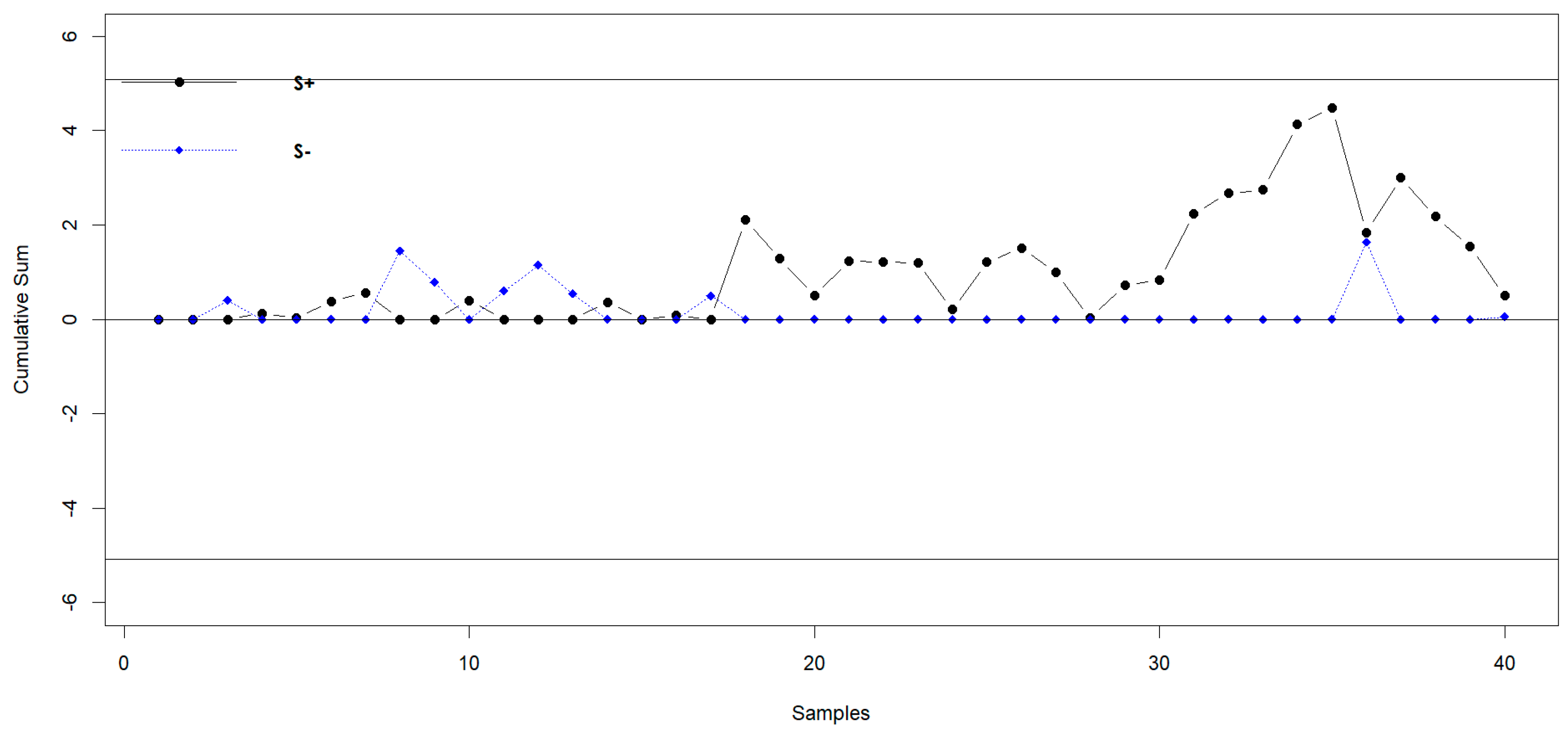
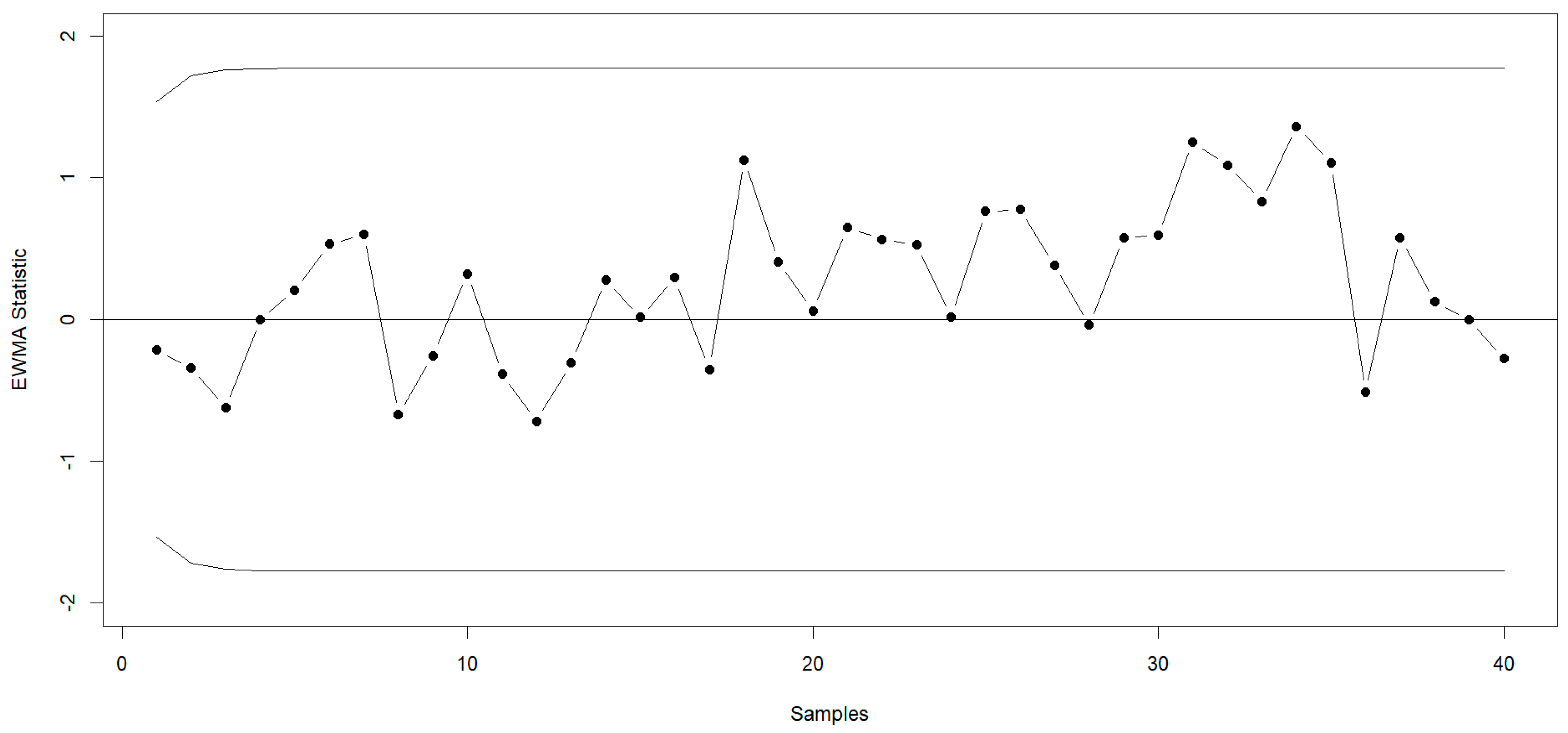
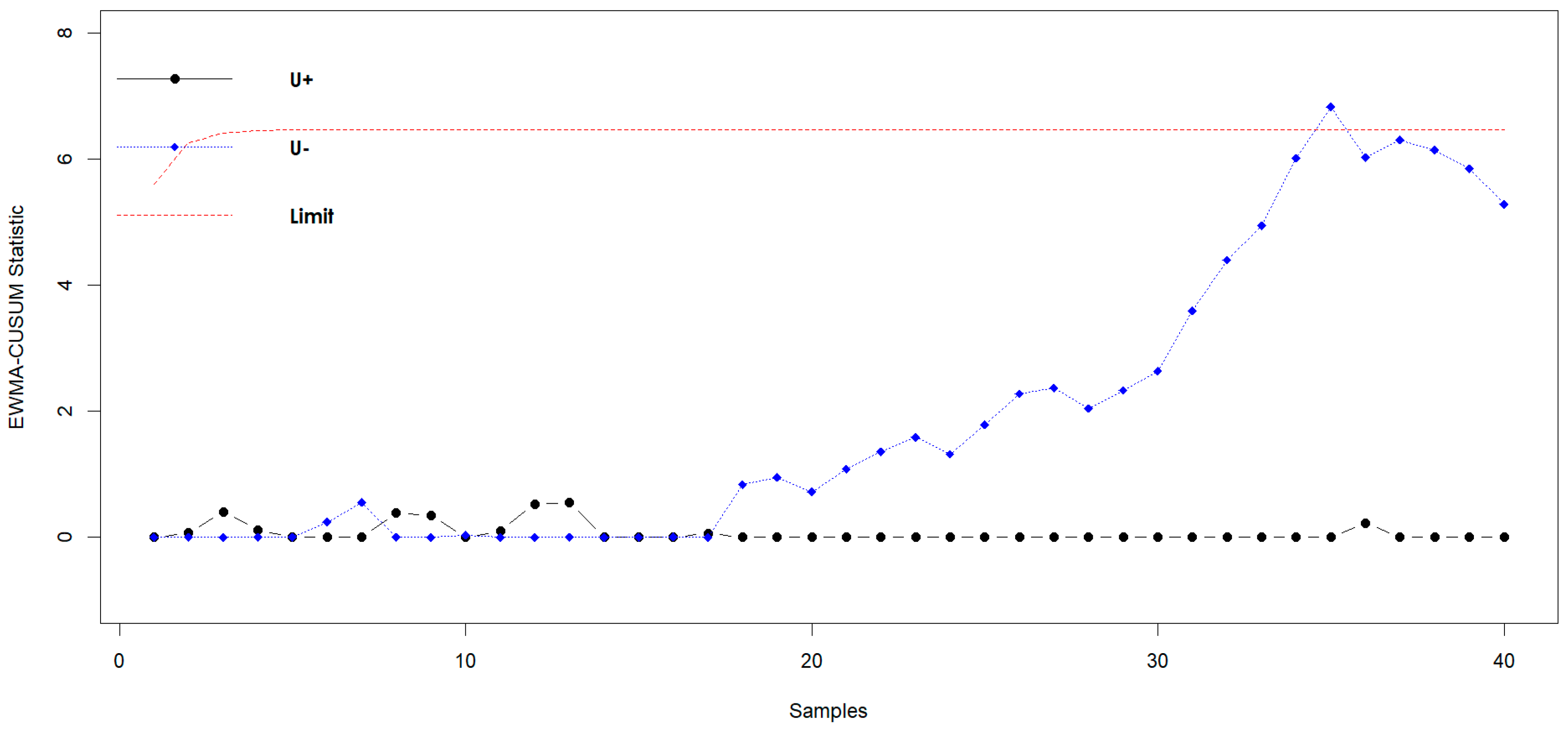
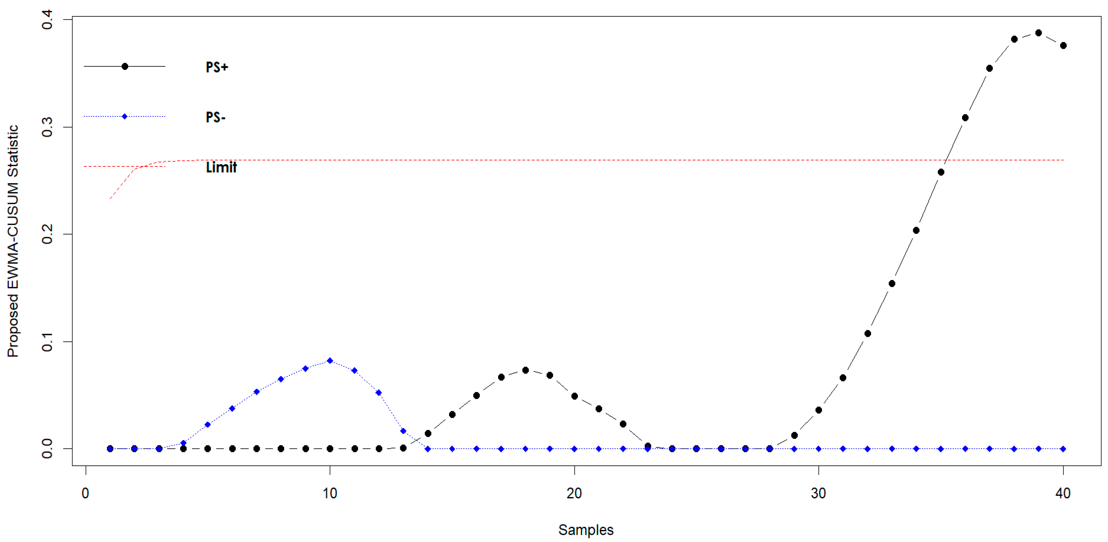
5.12. Graphical Presentation

To provide a comprehensive comparison between the proposed scheme and other existing counterparts, graphical displays in the form of ARL curves have been created. Five selective graphs representing different charts and schemes (discussed in Table 1, Table 2, Table 3, Table 4, Table 5, Table 6, Table 7, Table 8, Table 9, Table 10, Table 11, Table 12, Table 13, Table 14, Table 15, Table 16, Table 17, Table 18, Table 19, Table 20, Table 21, Table 22, Table 23, Table 24, Table 25, Table 26, Table 27 and Table 28) are presented as Figure 2, Figure 3, Figure 4, Figure 5 and Figure 6. In Figure 2, Figure 3, Figure 4, Figure 5 and Figure 6, the term “RR CUSUM (EWMA)” refers to run rules-based CUSUM (EWMA) schemes, while the remaining terms and symbols are self-explanatory.

Upon examining the ARL curves of the various schemes under investigation, it is observed that the ARL curves of the proposed schemes consistently fall on the lower side. This indicates that the proposed scheme demonstrates dominance over the other schemes. Notably, for smaller values of the shift parameter “$\delta$“, the difference between the ARL of the proposed scheme and the other schemes is more pronounced. However, as the shift parameter increases to large values, this difference tends to diminish. For larger values of the shift parameter, the ARL curve of the proposed chart appears close to the ARL curves of some other charts, suggesting relatively similar performance of the proposed chart for larger shifts.

In compendium, it can be inferred that the proposed scheme is generally effective in detecting small and moderate shifts, showcasing its superiority over other schemes. However, for larger shifts, the performance of the proposed scheme is comparatively similar as compared to some of the other schemes under investigation.

6. Real-Life Application

In order to provide practical insight into the proposed scheme, it is beneficial to demonstrate its application using real-life data sets. Drawing inspiration from previous studies conducted by Lucas and Crosier [7], Riaz et al. [9], and Zaman et al. [12], we present an illustrative example to showcase the implementation of the proposed scheme in a real-life scenario.

For this purpose, we generate a data set consisting of 40 observations. The first 20 observations represent the in-control situation, where the values are generated from a long-tailed symmetric probability distribution with a shape parameter of 2.5, a mean of 0, and a standard deviation of 1 (i.e., $X_j~LTS\left(p=2.5,\theta =0,\lambda =1\right)$). The subsequent 20 observations represent an out-of-control situation, where a small shift is introduced in the process, resulting in values generated from long-tailed symmetric probability distribution with a shape parameter of 2.5, a mean of 0.5, and a standard deviation of 1 (i.e., $X_j~LTS\left(p=2.5,\theta =0.5,\lambda =1\right)$).

To assess the performance of different control chart methods, namely the classic CUSUM, the classic EWMA, mixed EWMA-CUSUM, and the proposed scheme, we apply these methods to the generated data set. The parameter values chosen for the classic CUSUM scheme are $K$ = 0.5 and $H$ = 5.09; for the classic EWMA scheme values are $\phi$ = 0.5 and $W$ = 3.072, for the mixed EWMA-CUSUM scheme values are $\phi$ = 0.5, $k_E^{\ast }$ = 0.5, and $h_E^{\ast }$ = 11.2, and for the proposed scheme, values are ${\phi }_r$ = 0.5, $k_R^{\ast }$ = 0.5, and $h_R^{\ast }$ = 7.77. These parameter selections are made to ensure that the average run length under the in-control condition (ARL₀) is equal to 500.

Table 29. Application example of proposed scheme using ${\phi }_r$ = 0.5, $k_R^{\ast }$ = 0.5, and $h_R^{\ast }$ = 7.77 at ARL₀ = 500.

Sample No.	${\mathit{y}}_{\mathit{j}}$	${\mathit{R}}_{\mathit{j}}$	${\mathit{K}}_{{\mathit{R}}_{\mathit{j}}}$	$\mathit{P}{\mathit{S}}_{\mathit{j}}^{+}$	$\mathit{P}{\mathit{S}}_{\mathit{j}}^{-}$	${\mathit{H}}_{{\mathit{R}}_{\mathit{j}}}$
1	−0.4349	0.0063	0.0150	0	0	0.2333
2	−0.4739	0.0032	0.0168	0	0	0.2608
3	−0.9013	−0.0085	0.0172	0	0	0.2673
4	0.6214	−0.0226	0.0173	0	0.0053	0.2689
5	0.4051	−0.0346	0.0173	0	0.0225	0.2692
6	0.8579	−0.0326	0.0173	0	0.0378	0.2693
7	0.6719	−0.0325	0.0173	0	0.0530	0.2694
8	−1.9477	−0.0293	0.0173	0	0.0650	0.2694
9	0.1620	−0.0273	0.0173	0	0.0749	0.2694
10	0.8997	−0.0248	0.0173	0	0.0824	0.2694
11	−1.0975	−0.0078	0.0173	0	0.0729	0.2694
12	−1.0499	0.0032	0.0173	0	0.0523	0.2694
13	0.1022	0.0183	0.0173	0.0009	0.0167	0.2694
14	0.8610	0.0306	0.0173	0.0142	0	0.2694
15	−0.2477	0.0354	0.0173	0.0323	0	0.2694
16	0.5758	0.0351	0.0173	0.0500	0	0.2694
17	−1.0004	0.0343	0.0173	0.0670	0	0.2694
18	2.6021	0.0239	0.0173	0.0735	0	0.2694
19	−0.3164	0.0124	0.0173	0.0686	0	0.2694
20	−0.2892	−0.0023	0.0173	0.0490	0	0.2694
21	1.2362	0.0058	0.0173	0.0375	0	0.2694
22	0.4803	0.0029	0.0173	0.0231	0	0.2694
23	0.4866	−0.0033	0.0173	0.0024	0	0.2694
24	−0.4928	−0.0101	0.0173	0	0	0.2694
25	1.5063	−0.0135	0.0173	0	0	0.2694
26	0.7896	−0.0110	0.0173	0	0	0.2694
27	−0.0107	−0.0059	0.0173	0	0	0.2694
28	−0.4599	0.0168	0.0173	0	0	0.2694
29	1.1920	0.0297	0.0173	0.0123	0	0.2694
30	0.6065	0.0409	0.0173	0.0359	0	0.2694
31	1.9126	0.0477	0.0173	0.0663	0	0.2694
32	0.9250	0.0584	0.0173	0.1074	0	0.2694
33	0.5797	0.0641	0.0173	0.1542	0	0.2694
34	1.8840	0.0666	0.0173	0.2034	0	0.2694
35	0.8481	0.0717	0.0173	0.2579	0	0.2694
36	−2.1358	0.0679	0.0173	0.3084	0	0.2694
37	1.6618	0.0634	0.0173	0.3545	0	0.2694
38	−0.3279	0.0447	0.0173	0.3818	0	0.2694
39	−0.1319	0.0233	0.0173	0.3878	0	0.2694
40	−0.5497	0.0054	0.0173	0.3759	0	0.2694

provides a comprehensive overview of the computations conducted to assess the performance of our proposed control chart scheme. The table includes all the essential parameters that were calculated for a random sample comprising 40 observations. These calculations play a crucial role in evaluating the effectiveness and reliability of our control chart scheme in monitoring and detecting any potential deviations from the established control limits.

When we examined the classic CUSUM and EWMA schemes individually, as depicted in Figure 7 and Figure 8, they failed to detect any out-of-control situations within the given data set. This suggests that relying solely on these traditional methods may lead to undetected anomalies and a higher risk of quality issues going unnoticed. However, when we applied the mixed EWMA-CUSUM scheme on the data set, as illustrated in Figure 9, it did indicate an out-of-control signal at sample 35. However, rather than indicating further out-of-control signals, the control chart returned to a normal state starting from sample 36 onwards. This signifies that our proposed scheme has an advantage over the classic CUSUM, EWMA, and mixed EWMA-CUSUM schemes, as it successfully identified an abnormal pattern in the data.

In contrast, by analyzing the data presented in Table 29 and studying Figure 10, it becomes evident that the control chart scheme we proposed has proven to be effective in identifying out-of-control signals. Specifically, at samples 36, 37, 38, 39, and 40, our scheme detected a total of five instances of out-of-control signals. This is a significant finding that showcases the capability of our proposed scheme in detecting deviations from the expected control limits.

These findings provide compelling evidence of the superiority of our proposed control chart scheme over the traditional methods. Moreover, these results align perfectly with the conclusions presented in Section 5, further validating the effectiveness and reliability of our proposed approach.

7. Summary and Conclusions

In this study, we addressed the critical challenge of process monitoring in situations where the underlying distribution deviates from normality. Our primary objective was to develop a robust mixed EWMA-CUSUM control chart that would demonstrate superior sensitivity to minor or moderate deviations in process parameters while still addressing larger variations. The innovation in our approach lies in the integration of a robust estimator based on order statistics, utilizing the generalized least square (GLS) technique pioneered by Lloyd. This integration significantly enhances the chart’s robustness and minimizes estimator variance, even in the presence of non-normality. This research has made a substantial contribution to the field by providing a novel, mixed EWMA-CUSUM control chart tailored for monitoring processes with symmetric but non-normal distributions.

This research study was motivated by the recognition that traditional control charts, including Shewhart control charts, while effective at detecting significant shifts, may fall short in capturing smaller variations, particularly when the underlying distribution deviates from normality. By integrating a robust estimator based on order statistics and leveraging the GLS technique pioneered by Lloyd, our approach addresses this limitation head-on. This novel chart design significantly improves its ability to detect subtle shifts, setting it apart from similar methods. The incorporation of these statistical techniques enhances the robustness of the chart, making it applicable to a wide range of processes characterized by symmetric but non-normal distributions. The comparative analysis undertaken in this study, involving eleven well-established control charts, underscored the superior performance of our proposed chart when it comes to detecting small to moderate shifts. This is in line with our primary objective of achieving higher sensitivity for smaller variations. Moreover, the proposed chart’s performance for larger shifts remained comparable to existing alternatives, demonstrating its versatility and effectiveness across a broad spectrum of process variations.

In conclusion, this research not only introduced a practical solution to the challenge of monitoring non-normally distributed processes but also expanded the scope of control chart applications. The mixed EWMA-CUSUM control chart developed in this study represents a valuable tool for industries where maintaining quality standards and operational efficiency are paramount. Its enhanced sensitivity to smaller variations can lead to timely interventions, ultimately contributing to improved process performance and product quality.

References

1. Shewhart, W.A. The Economic Control of Quality of Manufactured Product. J. R. Stat. Soc. 1932, 95, 546. [Google Scholar] [CrossRef]
2. Montgomery, D.C. Introduction to Statistical Quality Control; John Wiley & Sons: Hoboken, NJ, USA, 2020. [Google Scholar]
3. Page, E.S. Continuous Inspection Schemes. Biometrika 1954, 41, 100–115. [Google Scholar] [CrossRef]
4. Roberts, S.W. Control Chart Tests Based on Geometric Moving Averages. Technometrics 2000, 42, 97–101. [Google Scholar] [CrossRef]
5. Lucas, J.M. Combined Shewhart-CUSUM Quality Control Schemes. J. Qual. Technol. 1982, 14, 51–59. [Google Scholar] [CrossRef]
6. Lucas, J.M.; Saccucci, M.S. Exponentially Weighted Moving Average Control Schemes: Properties and Enhancements. Technometrics 1990, 32, 1–12. [Google Scholar] [CrossRef]
7. Lucas, J.M.; Crosier, R.B. Fast Initial Response for CUSUM Quality-Control Schemes: Give Your CUSUM A Head Start. Technometrics 2000, 42, 102–107. [Google Scholar] [CrossRef]
8. Steiner, S.H. EWMA Control Charts with Time-Varying Control Limits and Fast Initial Response. J. Qual. Technol. 1999, 31, 75–86. [Google Scholar] [CrossRef]
9. Riaz, M.; Abbas, N.; Does, R.J.M.M. Improving the Performance of CUSUM Charts. Qual. Reliab. Eng. Int. 2011, 27, 415–424. [Google Scholar] [CrossRef]
10. Abbas, N.; Riaz, M.; Does, R.J.M.M. Enhancing the Performance of EWMA Charts. Qual. Reliab. Eng. Int. 2011, 27, 821–833. [Google Scholar] [CrossRef]
11. Abbas, N.; Riaz, M.; Does, R.J.M.M. Mixed Exponentially Weighted Moving Average-Cumulative Sum Charts for Process Monitoring. Qual. Reliab. Eng. Int. 2013, 29, 345–356. [Google Scholar] [CrossRef]
12. Zaman, B.; Riaz, M.; Abbas, N.; Does, R.J.M.M. Mixed Cumulative Sum-Exponentially Weighted Moving Average Control Charts: An Efficient Way of Monitoring Process Location. Qual. Reliab. Eng. Int. 2015, 31, 1407–1421. [Google Scholar] [CrossRef]
13. Zaman, B.; Abbas, N.; Riaz, M.; Lee, M.H. Mixed CUSUM-EWMA Chart for Monitoring Process Dispersion. Int. J. Adv. Manuf. Technol. 2016, 86, 3025–3039. [Google Scholar] [CrossRef]
14. Abid, M.; Mei, S.; Nazir, H.Z.; Riaz, M.; Hussain, S. A Mixed HWMA-CUSUM Mean Chart with an Application to Manufacturing Process. Qual. Reliab. Eng. Int. 2021, 37, 618–631. [Google Scholar] [CrossRef]
15. Abid, M.; Mei, S.; Nazir, H.Z.; Riaz, M.; Hussain, S.; Abbas, Z. A Mixed Cumulative Sum Homogeneously Weighted Moving Average Control Chart for Monitoring Process Mean. Qual. Reliab. Eng. Int. 2021, 37, 1758–1771. [Google Scholar] [CrossRef]
16. Riaz, M.; Khaliq, Q.-U.-A.; Gul, S. Mixed Tukey EWMA-CUSUM Control Chart and Its Applications. Qual. Technol. Quant. Manag. 2017, 14, 378–411. [Google Scholar] [CrossRef]
17. Ahmed, A.; Sanaullah, A.; Hanif, M. A Robust Alternate to the HEWMA Control Chart under Non-Normality. Qual. Technol. Quant. Manag. 2020, 17, 423–447. [Google Scholar] [CrossRef]
18. Nazir, H.; Abid, M.; Akhtar, N.; Riaz, M.; Qamar, S. An Efficient Mixed-Memory-Type Control Chart for Normal and Non-Normal Processes. Sci. Iran. 2021, 28, 1736–1749. [Google Scholar] [CrossRef]
19. Aslam, M. A Mixed EWMA—CUSUM Control Chart for Weibull-Distributed Quality Characteristics. Qual. Reliab. Eng. Int. 2016, 32, 2987–2994. [Google Scholar] [CrossRef]
20. Rao, G.S.; Aslam, M.; Rasheed, U.; Jun, C.-H. Mixed EWMA–CUSUM chart for COM-Poisson distribution. J. Stat. Manag. Syst. 2020, 23, 511–527. [Google Scholar] [CrossRef]
21. Hussain, S.; Wang, X.; Ahmad, S.; Riaz, M. On a class of mixed EWMA-CUSUM median control charts for process monitoring. Qual. Reliab. Eng. Int. 2020, 36, 910–946. [Google Scholar] [CrossRef]
22. Sales, L.O.F.; Pinho, A.L.S.; Bourguignon, M.; Medeiros, F.M.C. Control charts for monitoring the median in non-negative asymmetric data. Stat. Methods Appl. 2022, 31, 1037–1068. [Google Scholar] [CrossRef]
23. Guh, R.S.; Hsieh, Y.C. A neural network-based model for abnormal pattern recognition of control charts. Comput. Ind. Eng. 1999, 36, 97–108. [Google Scholar] [CrossRef]
24. Zan, T.; Liu, Z.; Wang, H.; Wang, M.; Gao, X. Control chart pattern recognition using the convolutional neural network. J. Intell. Manuf. 2020, 31, 703–716. [Google Scholar] [CrossRef]
25. Chen, S.; Yu, J. Deep recurrent neural network-based residual control chart for autocorrelated processes. Qual. Reliab. Eng. Int. 2019, 35, 2687–2708. [Google Scholar] [CrossRef]
26. Pugh, G.A. Synthetic neural networks for process control. Comput. Ind. Eng. 1989, 17, 24–26. [Google Scholar] [CrossRef]
27. Huber, P.J. Robust Statistics: Huber/Robust Statistics; Wiley Series in Probability and Statistics; John Wiley & Sons, Inc.: Hoboken, NJ, USA, 1981. [Google Scholar] [CrossRef]
28. Hampel, F.; Ronchetti, E.; Rousseeuw, P.J.; Stahel, W.A. Robust Statistics: The Approach Based on Influence Functions. J. R. Stat. Society. Ser. A (Gen.) 1987, 150, 281. [Google Scholar] [CrossRef]
29. Lloyd, E.H. Least-Squares Estimation of Location and Scale Parameters using Order Statistics. Biometrika 1952, 39, 88–95. [Google Scholar] [CrossRef]
30. Tiku, M.L.; Kumra, S. Expected Values and Variances and Covariances of Order Statistics for a Family of Symmetric Distributions (Student’st). Sel. Tables Math. Stat. 1985, 8, 141–270. [Google Scholar]
31. Vaughan, D.C. Expected Values, Variances and Covariances of Order Statistics for Student’s t-Distribution with Two Degrees of Freedom. Commun. Stat.—Simul. Comp. 1992, 21, 391–404. [Google Scholar] [CrossRef]
32. Yashchin, E. Weighted Cumulative Sum Technique. Technometrics 1989, 31, 321–338. [Google Scholar] [CrossRef]
33. Jiang, W.; Shu, L.; Apley, D.W. Adaptive CUSUM Procedures with EWMA-Based Shift Estimators. IIE Trans. 2008, 40, 992–1003. [Google Scholar] [CrossRef]
34. Zaman, B.; Lee, M.H.; Riaz, M.; Abujiya, M.R. An Adaptive EWMA Scheme-Based CUSUM Accumulation Error for Efficient Monitoring of Process Location. Qual. Reliab. Eng. Int. 2017, 33, 2463–2482. [Google Scholar] [CrossRef]
Figure 1. The probability density function of LTS at p = 2.5, 5, 10, and 20.
Mathematics 11 04157 g001
Figure 2. ARL comparisons of proposed mixed EWMA-CUSUM, classic CUSUM, and classic EWMA at ARL0 = 168.
Mathematics 11 04157 g002
Figure 3. ARL comparisons of proposed mixed EWMA-CUSUM, FIR-CUSUM with S0 = 1 and 2, FIR-EWMA with 25% and 50% head start at ARL0 = 500.
Mathematics 11 04157 g003
Figure 4. ARL comparisons of proposed mixed EWMA-CUSUM, RR-CUSUM with Scheme 1 and 2, RR-EWMA with Scheme 1 and 2 at ARL0 = 500.
Mathematics 11 04157 g004
Figure 5. ARL comparisons of proposed mixed EWMA-CUSUM, weighted CUSUM, adaptive EWMA with scheme I and II at ARL0 = 500.
Mathematics 11 04157 g005
Figure 6. ARL comparisons of proposed mixed EWMA-CUSUM, Shewhart Scheme, adaptive CUSUM, mixed EWMA-CUSUM at ARL0 = 500.
Mathematics 11 04157 g006
Figure 7. The CUSUM scheme for the simulated data with K = 0.5 and H = 5.09 at ARL0 = 500.
Mathematics 11 04157 g007
Figure 8. The EWMA scheme for the simulated data with φ = 0.5 and W = 3.072 at ARL0 = 500.
Mathematics 11 04157 g008
Figure 9. The proposed mixed EWMA−CUSUM scheme for the simulated data with φ r = 0.5, k R = 0.5, and h R = 7.77 at ARL0 = 500.
Mathematics 11 04157 g009
Figure 10. The proposed mixed EWMA−CUSUM scheme for the simulated data with φ = 0.5, k E = 0.5, and h E = 11.2 at ARL0 = 500.
Mathematics 11 04157 g010