Application of Fractional Differential Model in Image Enhancement of Strong Reflection Surface

Abstract

Combined with advanced fractional differential mask operation, this paper used a fractional differential to normalize the 5 × 5 mask and conducted experiments to select fractional v = 0.7 to determine the equation. The position of the center of the light band was obtained by the gray centroid method, and the center of the light band was enhanced by the fractional differential algorithm. Three samples of hard disk substrate, roller, and printed circuit board were selected. The traditional processing was compared to the fractional differential algorithm in this paper, and several advanced algorithms were compared with the algorithm in this paper. Experimental data showed that fractional differential enhancement can effectively improve the accuracy of extracting the center of light fringes. It can be found that the average error of extracting the center by fractional differential processing was relatively small, and the image outline was clearer.

1. Introduction

In recent years, fractional differential theory has gradually attracted great attention from engineering and technical personnel, and it has been applied to electrochemistry [1], material mechanics [2], fluid field theory [3], control theory [4,5], electromagnetic field theory [6], biomedicine [7], and signal processing [8]. Fractional differential theory has achieved fruitful research results. It was found that fractional calculus theory is suitable for studying uncertain signals with nonlinear, non-causal, and non-stationary characteristics. Therefore, many classical algorithms in fractional calculus theory are very suitable for modern signal analysis and processing. In this paper, the fractional differential model was applied to the image enhancement of the on-line structured light vision measurement of strongly reflective surfaces.

In the process of light stripe image enhancement, the key is to enhance the speckle noise highlighted by the sense of particles while preserving the effective fringe image area with continuous gray scale. The commonly used image enhancement methods, both in the spatial domain and the frequency domain, have the contradiction of enhancing the high-frequency image and weakening the low-frequency part of the image [9]. For example, the histogram equalization method enhances the high-frequency component of the image, and the image histogram obeys the uniform distribution; however, the edge of the image is excessively cut and sharpened, which affects the identification of image information [10]. Later, the theory of Retinex proposed by Land [11] and others was widely used in image enhancement. The most classical algorithms are single-scale Retinex (SSR) [12] and multi-scale Retinex (MSR) [13]. They all use the Gaussian filter as a low-pass filter. Although the algorithm is simple, the image halo phenomenon is serious after enhancement, and the algorithm is based on the time-domain enhancement method. Additionally, the details are lost when processing the image. Andrivanov, Nikita et al., based on the deep double stochastic Gaussian model combined with nonlinear double stochastic filtering, achieved that the error of the recovered image was only 9% when only 50% of the image information was used [14]. Integer order differential gradient operators (first-order differential operators such as Sobel, Prewitt, and Canny operators; second-order differential operators such as Laplace operators) are usually effective in enhancing high-frequency details, but at the same time, low-frequency components are lost [15,16].

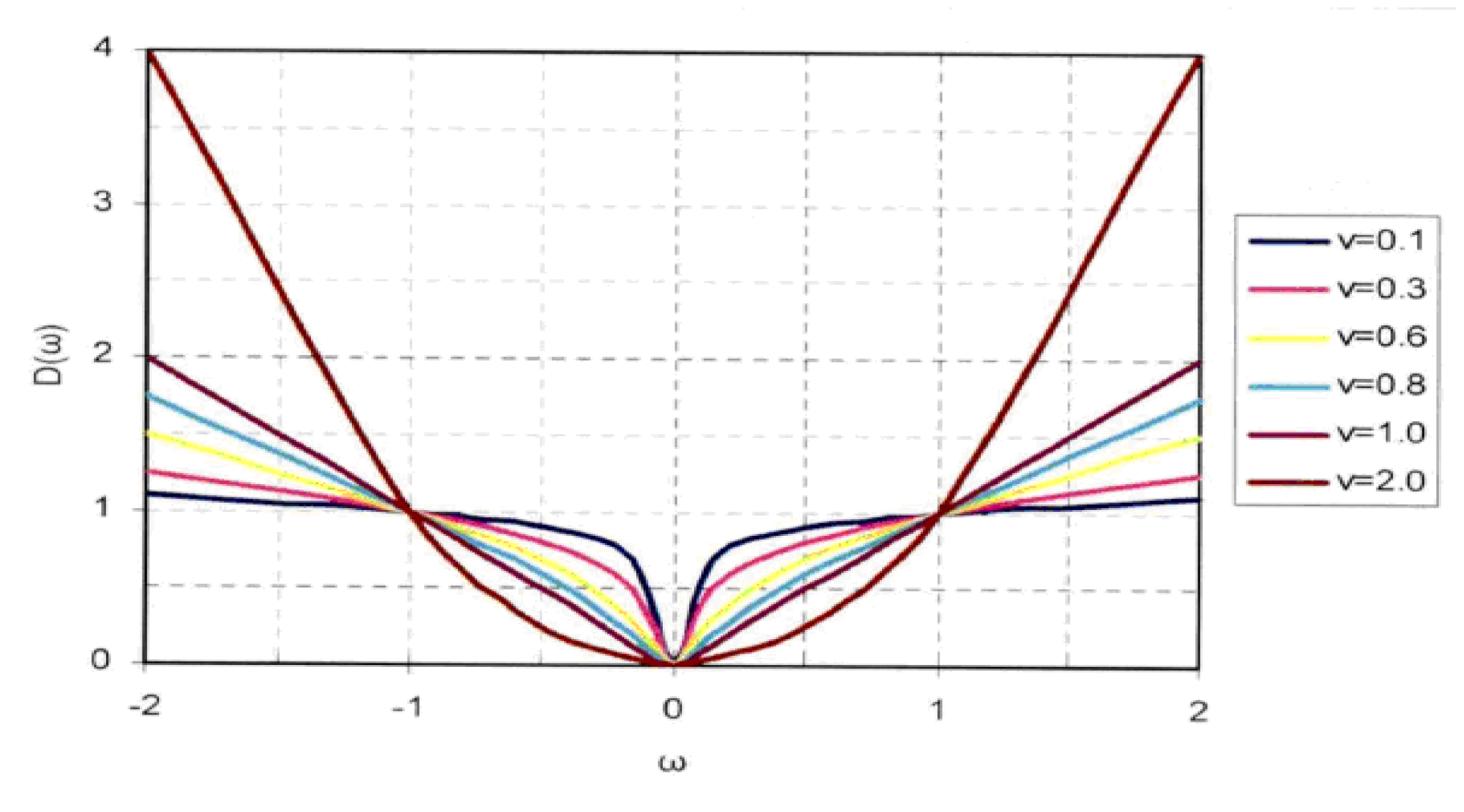
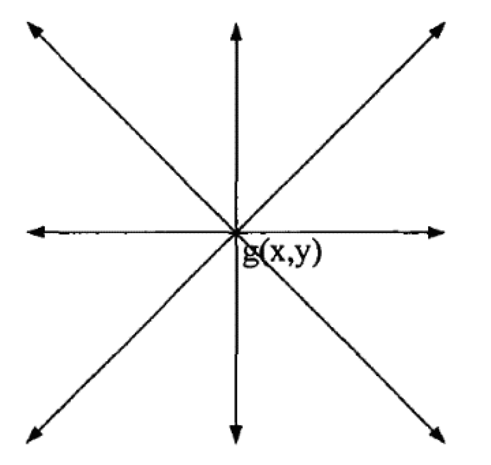
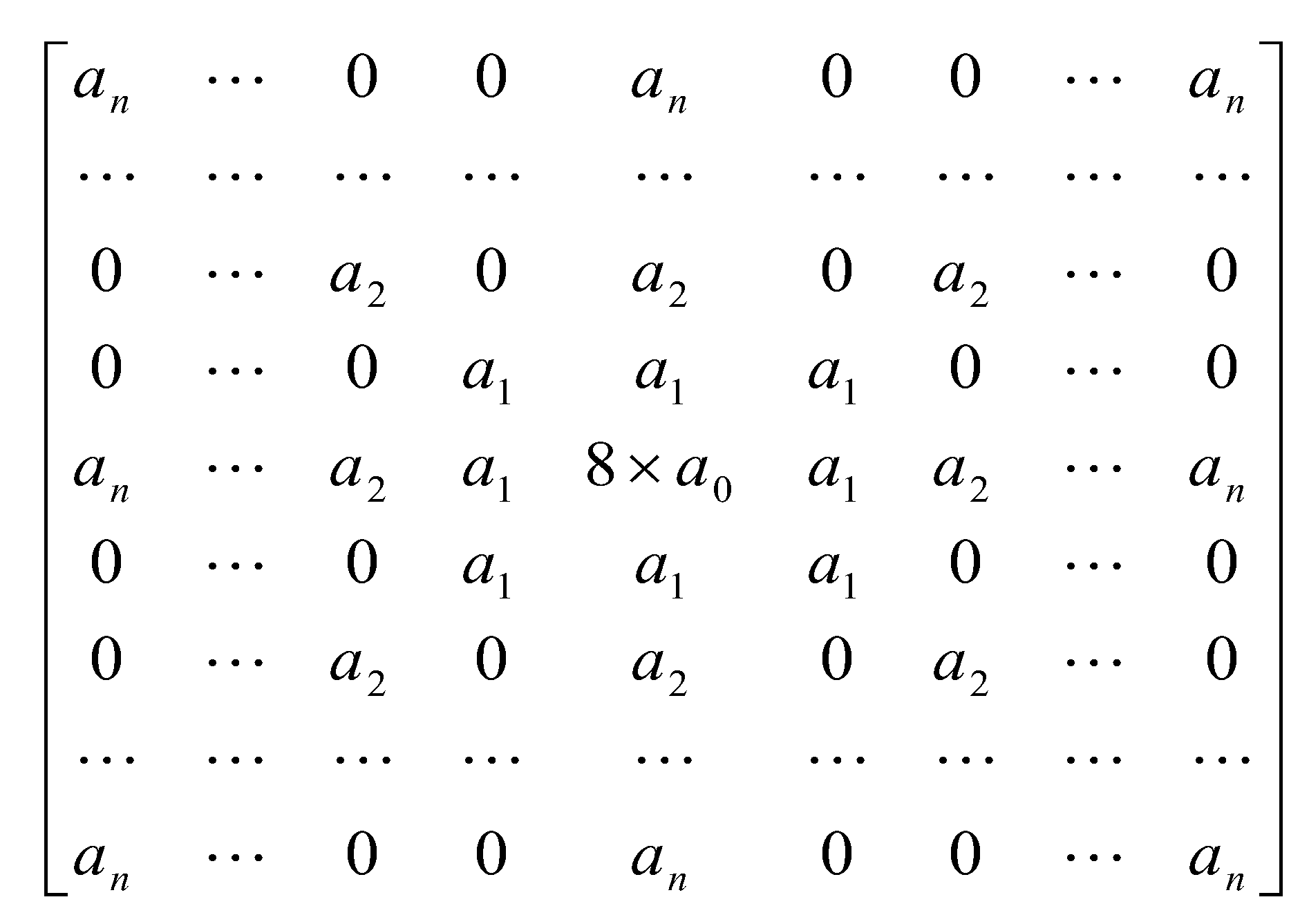
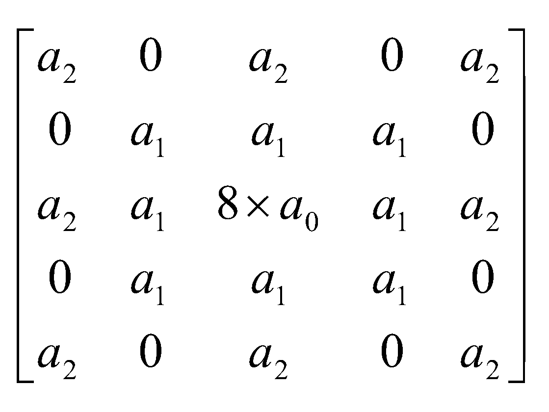
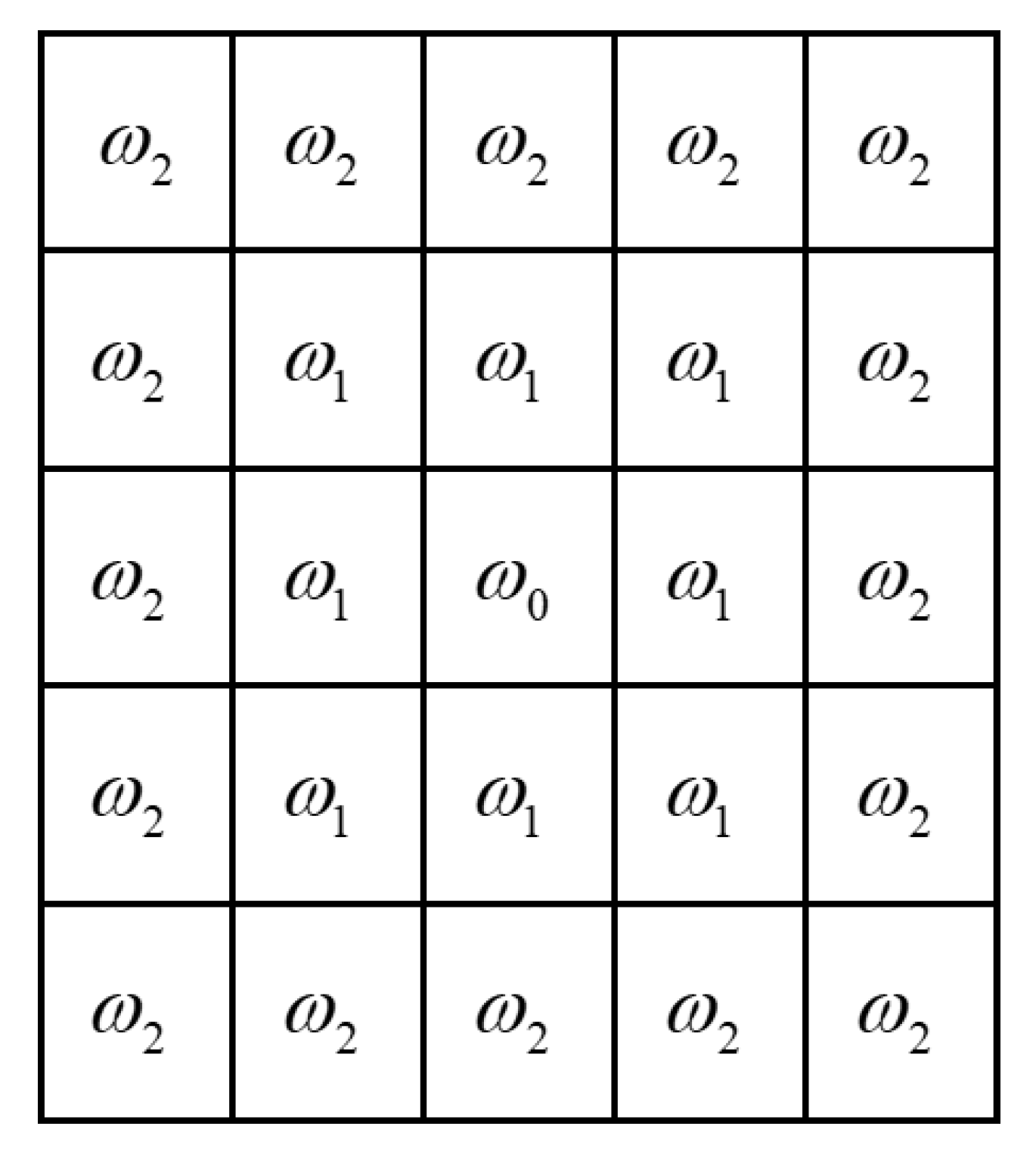
2. Fractional Differential Image Enhancement Model

Differential operation can enhance the high-frequency component of the signal. As shown in Figure 1, the second-order differential ($v=2$) increases the amplitude of the high-frequency part ($\omega >>1$), but the amplitude of the low-frequency part decreases significantly. The main difference between speckle noise on a strongly reflective surface and an effective continuous light stripe lies in the gray dispersion of image, that is, the difference between granular and continuous stripes. If the differential enhancement image processing method is used to highlight the graining characteristics of noise, then the high-frequency variation characteristics of the light stripe edge can be highlighted, but at the same time, it is hoped to effectively protect the information of low-frequency continuous fringes to extract the effective light stripe center by using the conventional gray center of the gravity method after removing the speckle noise of a strongly reflective surface. If the differential order is $0<v<1$, although the rise degree of the curve of the high-frequency part ($\omega >>1$) is lower than that of the integer order differential, then the amplitude of the low-frequency part is significantly higher than that of the integer order. Using fractional differentiation to process the image with a strong reflection speckle can highlight the edge of the image and enhance the texture information at the same time.

Under the Euclid measurement, the Grumwald-Letnikov fractional calculus is defined as [17,18,19]: $\forall v\in R$ ∀∈R. Rounding $v$ is $\left[v\right]$. If signal $f\left(t\right)\in \left[a,t\right](a<t,a\in R,t\in R)$ has a continuous $m+1$ derivative, when $v>0$, m takes at least the integer as $\left[v\right]$, then the $v$-order fractional derivative of $f\left(t\right)$ can be found in the following equation:

$${{\displaystyle D}}_G^{\mathrm{v}}s(t)\cong \underset{h\to 0}{\lim }{{\displaystyle f}}_h^{(v)}(t)\cong \underset{\begin{array}{l}h\to 0\\ nh=t-a\end{array}}{\lim }{{\displaystyle h}}^{-v}{\displaystyle \sum _{r=0}^{n-1}[\begin{array}{c}-v\\ r\end{array}]}f(t-rh)\cong \underset{n\to \infty }{\lim }\{\frac{{{\displaystyle (\frac{t-a}{v})}}^{-v}}{\mathsf{\Gamma }(-v)}{\displaystyle \sum _{r=0}^{n-1}\frac{\mathsf{\Gamma }(r-v)}{\mathsf{\Gamma }(r+1)}}f(t-\frac{r(t-a)}{n})\}$$

(1)

In the formula, $h$ stands for step size, $a$ represents the signal value, $n$ is the degree of continuous derivative, $t$ represents the time, and $r$ and $v$ represent integer order and fractional order, respectively.

Gamma Function:

$$\mathsf{\Gamma }(n)={\displaystyle \underset{0}{\overset{\infty }{\int }}{{\displaystyle e}}^{-t}}{{\displaystyle t}}^{n-1}dt=(n-1)!;[\begin{array}{c}-v\\ r\end{array}]=\frac{(-v)(-v+1)\dots (-v+r-1)}{r!}$$

(2)

To make $f_h^{\left(-v\right)}\left(t\right)$ the limit of approaches zero,$h\to 0$ when $n\to \infty$ and $h=\frac{t-a}{n}$. Namely, $n=\frac{t-a}{h}$. For image signals $f\left(x,y\right)$, the fractional partial differential is obtained for two independent variables $x$ and $y$, respectively, and the corresponding backward difference expression is obtained by the following [20,21,22,23],

$$\frac{{{\displaystyle \partial }}^{\mathrm{v}}f(x,y)}{\partial {{\displaystyle x}}^v}\approx f(x,y)+(-v)f(x-1,y)+\frac{(-v)(-v+1)}{2}f(x-2,y)+\dots +\frac{\mathsf{\Gamma }(-v+1)}{n!\mathsf{\Gamma }(-v+n+1)}f(x-n,y)$$

(3)

$$\frac{{{\displaystyle \partial }}^{\mathrm{v}}f(x,y)}{\partial {{\displaystyle y}}^v}\approx f(x,y)+(-v)f(x,y-1)+\frac{(-v)(-v+1)}{2}f(x,y-2)+\dots +\frac{\mathsf{\Gamma }(-v+1)}{n!\mathsf{\Gamma }(-v+n+1)}f(x,y-n)$$

(4)

Similarly, fractional differential expressions in six other directions such as $x$ negative direction, $y$ negative direction, and left-right diagonal direction can be obtained.

In Equations (3) and (4), the corresponding coefficients of the first $n+1$ term are equal, and the coefficients of the first $n+1$ term are as follows:

$${{\displaystyle a}}_0=1,{{\displaystyle a}}_1=-v,{{\displaystyle a}}_2=\frac{(-v)(-v+1)}{2},{{\displaystyle a}}_3=\frac{(-v)(-v+1)(-v+2)}{6},\dots ,{{\displaystyle a}}_n=\frac{\mathsf{\Gamma }(-v+2)}{n!\mathsf{\Gamma }(-v+n+1)}$$

(5)

Generally, for the image signal $f\left(x,y\right)$ of $M\times N$, M, N represents the height and width of the image. the image processing in the form of $m\times n$ is expressed as:

$$g(x,y)={\displaystyle \sum _{s=-a}^a{\displaystyle \sum _{t=-b}^{b}W(}}s,t)f(x+s,y+t)$$

(6)

where $a=\frac{m-1}{2}$, $b=\frac{n-1}{2}$ and $w\left(s,t\right)$ are strong reflection image filter mask operators. In order to obtain a complete enhanced image, all pixels whose distance between the center point of the mask and the edge of the original image $f$ is within $M-\frac{m-1}{2}$ and $N-\frac{n-1}{2}$ need to be fractional differential operation in eight directions one by one, as shown in Figure 2.

The same-sex filter in each direction constructed by Equation (5) can obtain the $\left(2n+1\right)\times \left(2n+1\right)$ fractional differential operator in eight symmetrical directions, as shown in Figure 3, and the elements not in the eight symmetrical operation directions are assigned a value of 0.

The fractional differential mask operator shown in Figure 3 has rotational isotropy and symmetry. In the application, by comprehensively analyzing the complexity of the differential operator and the effect of image enhancement, the operation scale is selected. In this paper, a $5\times 5$ operator as shown in Figure 4 was used as the strong reflection image filtering operator $w\left(s,t\right)$.

3. Fractional Differential Image Enhancement Model and Performance Evaluation

In order to make the best use of the autocorrelation of adjacent pixels and to make the weight of all pixels with a distance of 2 half of the original non-zero weight, the pixels with a weight of 0 were not omitted. At the same time, in order to make the pixel value of the enhanced image change within a certain range of the original pixel value, each item of the mask operator in Figure 4 was divided by $\left(8-12v+4v^2\right)$ for normalization. W₀, W₁, and W₂ were used to represent the values of 8a₀, a₁, and a₂ divided by $\left(8-12v+4v^2\right)$ in Figure 4, respectively. The result is shown in Formula (7). The value in the $5\times 5$ mask was replaced with W. The final $5\times 5$ mask operator is shown in Figure 5.

$${{\displaystyle \omega }}_0=\frac{2}{{{\displaystyle v}}^2-3\nu +2};{{\displaystyle \omega }}_1=\frac{-v}{{{\displaystyle 4\nu }}^2-12\nu +8};{{\displaystyle \omega }}_2=\frac{v}{16(v-2)}$$

(7)

The light bar images of three types of diffuse reflection samples were selected: PCB board, metal roller, and hard disk substrate. The image resolution was 1000 dpi and the size was 1200 pixels. The Sobel algorithm, Laplace algorithm, and fractional differential algorithm (order v = 0.5, v = 0.7 and v = 0.8) were selected for enhancement. The enhancement effects of different algorithms are shown in Figure 6, Figure 7 and Figure 8.

Table 1. Entropy and gradient values after enhanced processing by three algorithms.

	Information Entropy					Gradient
Image	Laplacian	Sobel	Differential			Laplacian	Sobel	Differential
			V = 0.5	V = 0.7	V = 0.8			V = 0.5	V = 0.7	V = 0.8
Pcb board	10.541	10.992	11.102	11.144	10.863	28.091	29.584	30.173	31.712	27.954
Roller	6.801	7.117	7.311	8.028	7.053	15.652	17.463	18.251	20.344	17.882
Hard disk base plate	6.154	7.206	7.494	7.779	7.196	14.396	15.461	17.512	18.197	16.996

shows the entropy and gradient values of the three images processed by different enhancement algorithms. The entropy and gradient values of the image after fractional differential enhancement were significantly higher than those of the other two algorithms, indicating that the fractional differential method retained more texture details after image enhancement. However, with the change of fractional order, it was found that when v = 0.7, the texture was significantly richer than that when v = 0.5, while when v = 0.8, there was excessive sharpening and enhancement. Therefore, v = 0.7 was selected in this paper.

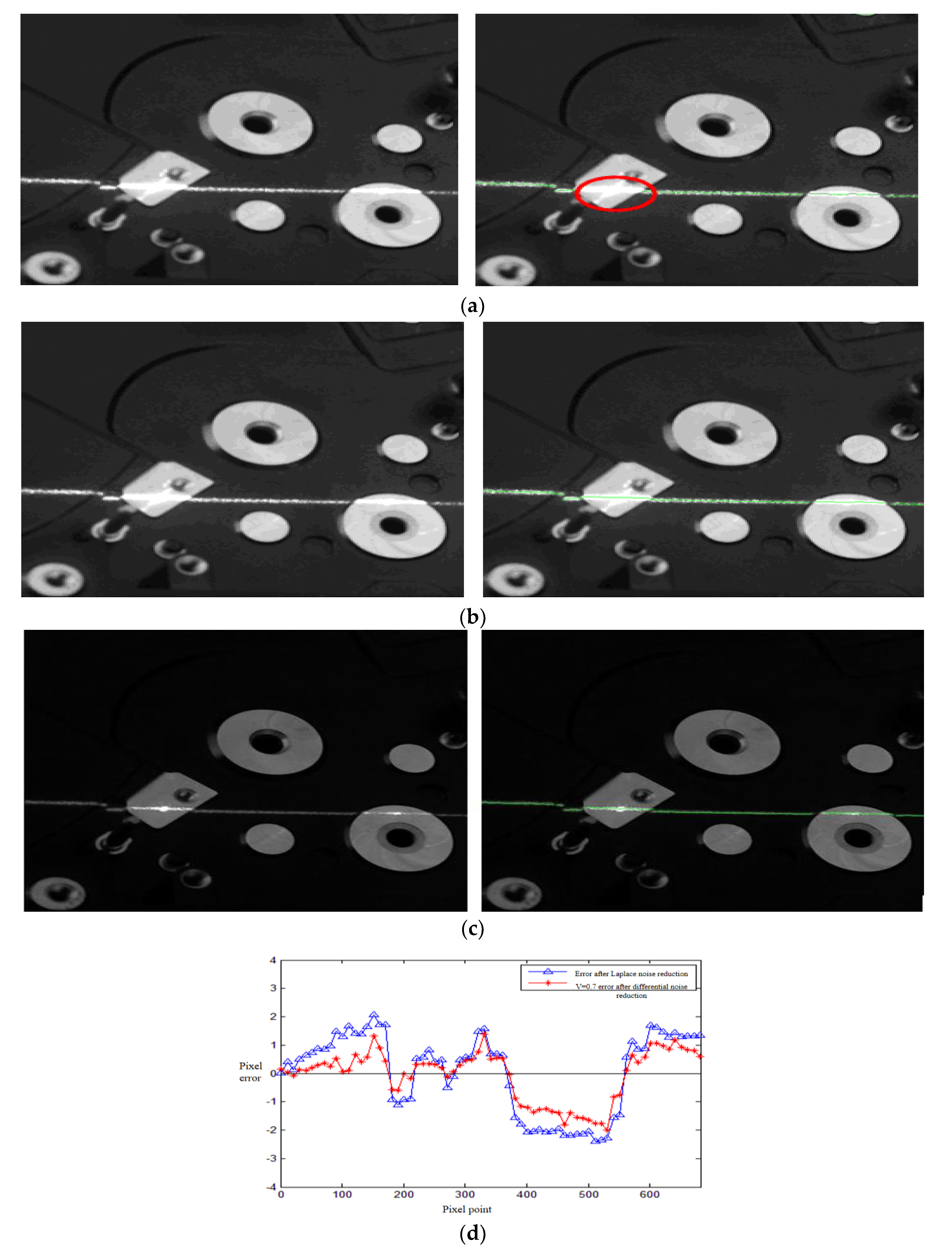
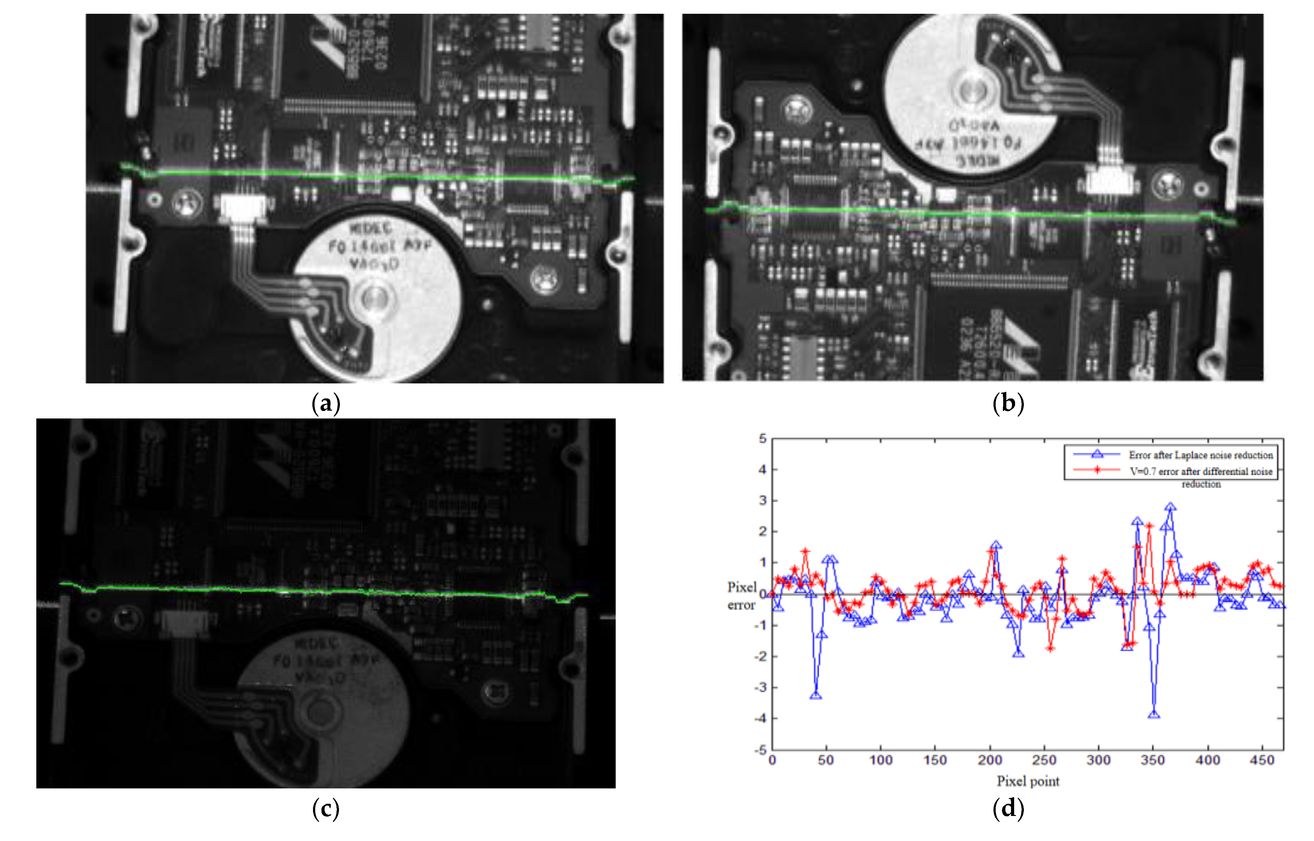
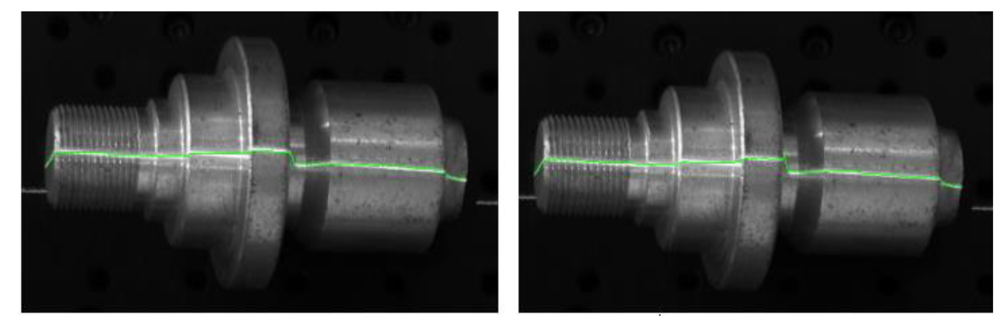
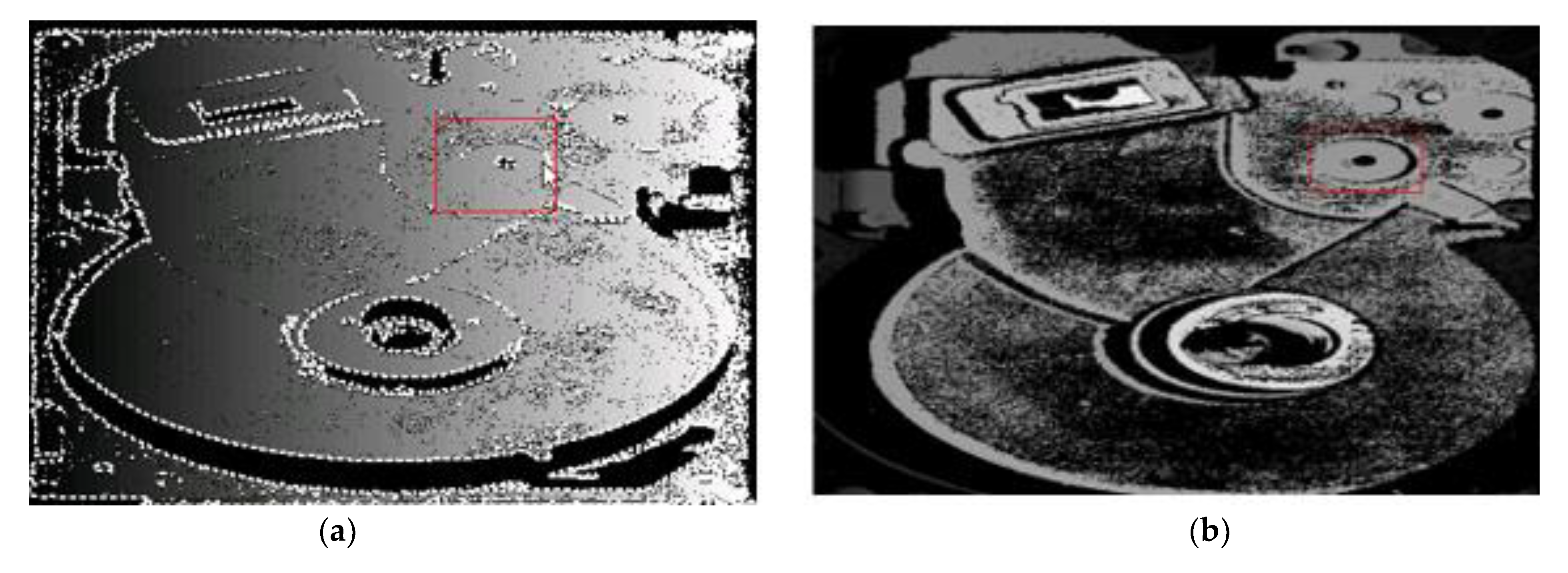
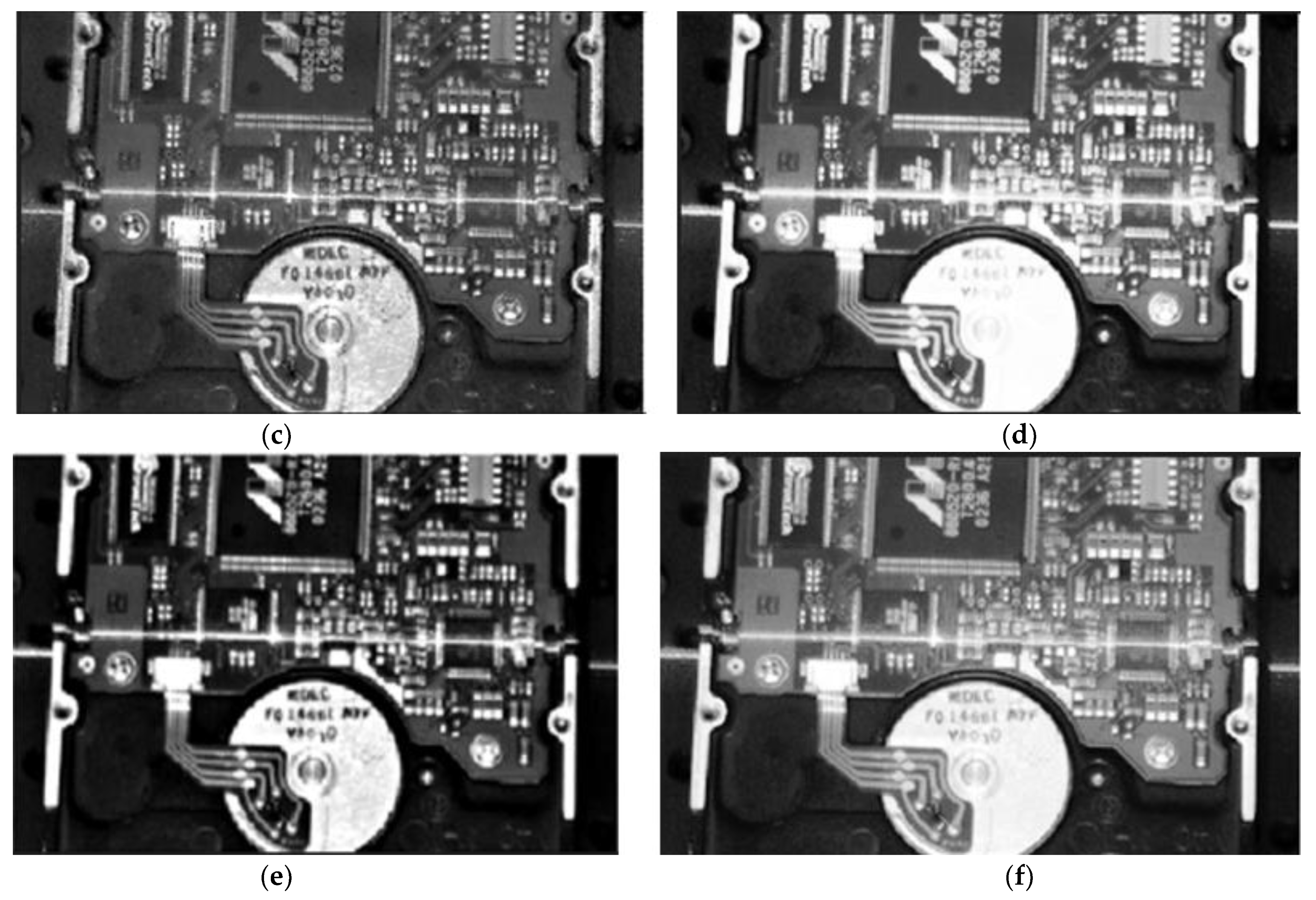
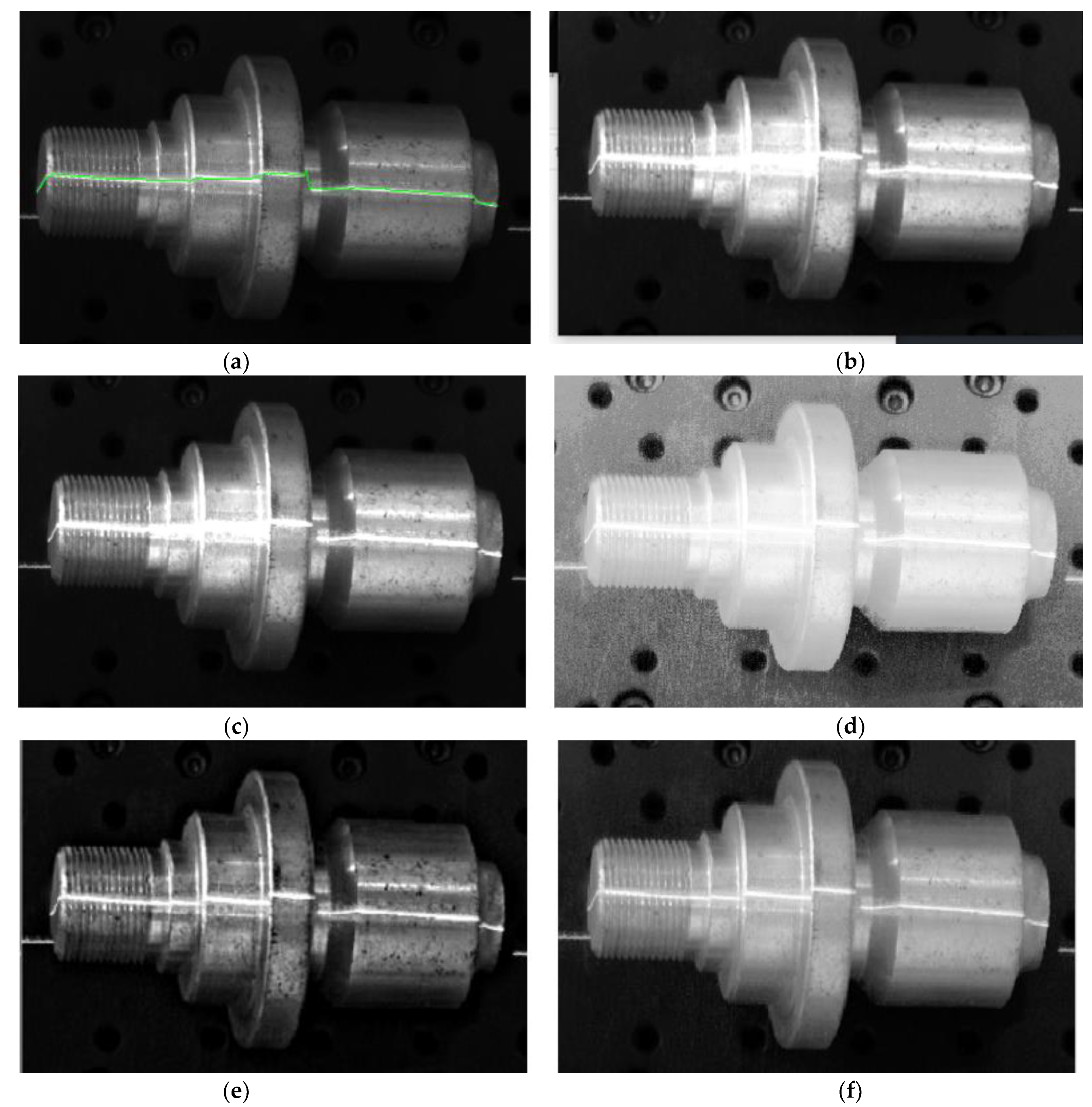
4. Experiment and Results of Structured Light Vision Measurement

After the light stripe image was enhanced by the fractional differential of the structured light vision measurement, the continuous light stripe and speckle noise were separated by connecting area statistics, and the speckle interference was removed to obtain the light stripe image. The effective fringe center was extracted using the gray center of gravity. The algorithm flow is shown in Figure 9. The center coordinates of the light bar image were obtained by the gray center of gravity method:

$$\left\{\begin{array}{c}{u}_j=j\\ v_i=\frac{{{\displaystyle \sum }}_{i}iG\left(i,j\right)}{{{\displaystyle \sum }}_{i}G\left(i,j\right)}\end{array}\right.$$

(8)

where G($i,j$) is the gray value of row i and column j in the light bar image, and ($u_j$,$v_j$) is the gray value of the extracted light bar image coordinates of the heart.

In order to verify the superiority of the method in this paper, a comparative experiment was set up to compare the algorithm in this paper with Laplacian denoising. Figure 10 shows the processing of the hard disk baseband highlight area by different algorithms. After denoising using the Laplace method, the center of light stripe was obtained by the gray center of gravity method. As shown in Figure 10a, the red ellipse marks the strong reflection area, and the extraction of the center of light stripe failed. The center of the light stripe was extracted by the fractional differentiation algorithm, as shown in Figure 10b. The image under the dark background dark light bar was taken and the light bar center was extracted, as shown in Figure 10c. The light bar center in the strong reflection area was extracted successfully. The performance comparison of extracting the light stripe center after the two methods is shown in Figure 10d. It can be seen from the figure that the error of the average extraction result of the fractional differential algorithm in the center of the hard disk baseband was reduced by 0.53 pixels compared to the Laplace algorithm. This proves that the algorithm in this paper had better performance when dealing with bright surfaces.

Images of the PCB board and roller were used for comparative experimental verification. Figure 11 shows the light stripe image in the strong reflection area of the PCB board. The center of the light stripe was extracted after the Steger method processing, as shown in Figure 11a; the center of the light stripe was extracted after fractional differential processing, as shown in Figure 11b; the center of the light stripe was extracted from the image under the dark background, as shown in Figure 11c; and the performance comparison is shown in Figure 11d. The average error of the extraction center of fractional differential processing was reduced by 0.61 pixels. Figure 12 shows the light stripe image in the strong reflection area of the roller. The center of the light stripe was extracted after the Steger method processing, as shown in Figure 12a; the center of the light stripe was extracted after fractional differential processing; as shown in Figure 12b; the center of the light stripe was extracted from the image under dark background, as shown in Figure 12c; and the performance comparison is shown in Figure 12d. The average error of the extraction center of fractional differential processing was reduced by 0.9 pixels.

After the strong reflection area was enhanced by fractional differentiation, the image outline was clearer, as shown in Figure 13.

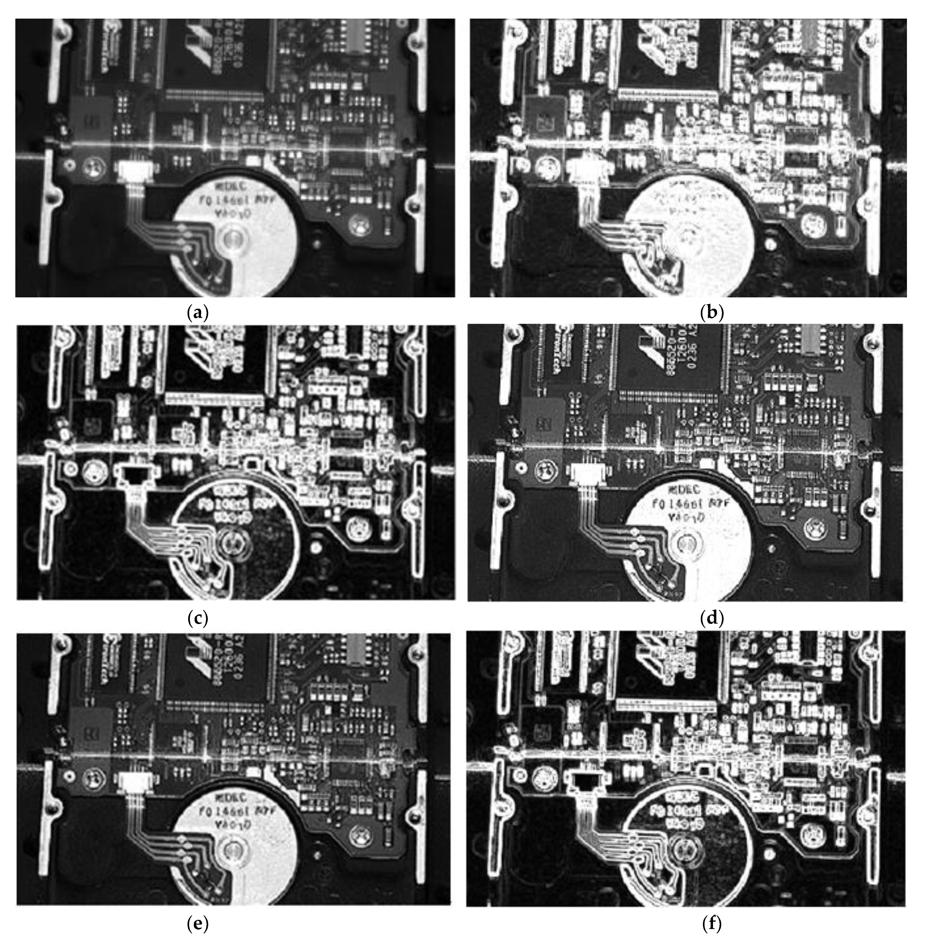
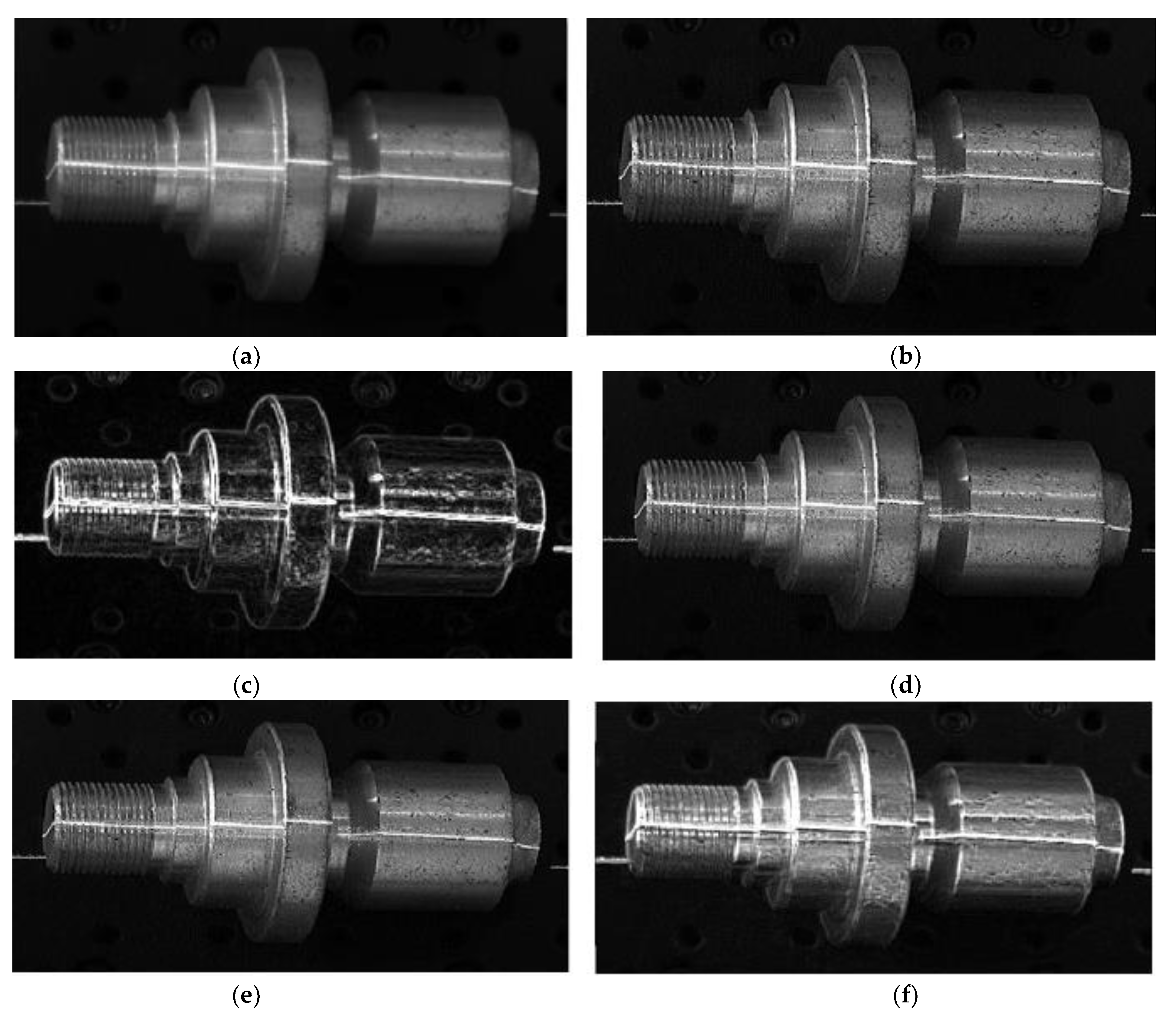
5. Comparative Experiment

In order to verify the effectiveness of the algorithm in this paper, five algorithms in recent years were selected, and a comparative experiment was performed by processing a PCB and metal roller. Ref. [24] firstly Fourier transformed the pixels in the spatial domain and then performed inverse Fourier transform to obtain a synthesized image. Ref. [25] selected the maximum value in each pixel channel to initialize the image light map, then refined the initial light map by strongly adding a structural prior, and finally synthesized the enhanced map according to the Retinex theory. Ref. [26] showed the pixel difference through a two-dimensional histogram, and used the image enhancement mapping function to process the histogram to export the image. Ref. [27] performed filtering based on the Laplacian operator, added a patch difference model, used the generalized Gamma distribution for parameter estimation, and determined the image enhancement algorithm according to the self-guided and external-guided characteristics of the filter. Ref. [28] adopted an improved AGC algorithm to achieve the CE of bright images with a new negative image strategy and used truncated CDF-modulated gamma correction to enhance dark images, which can alleviate local over-enhancement and structural distortion. The comparison results of PCB and metal roller processing are shown in Figure 14 and Figure 15.

6. Image Quality Assessment

Using NIQE (Natural Image Quality Evaluator), the design idea of this model was based on constructing a series of features for measuring image quality, and these features were used to fit a multivariate Gaussian model. These features were extracted from some simple and highly regular natural landscapes. This model actually measured the difference in the multivariate distribution of a test image, which was constructed with these features extracted from a series of normal natural images.

The NIQE quality evaluation model does not require the main performance evaluation score of the original image. It extracts image features from the original image library and then uses a multivariate Gaussian (MYG) model for modeling. Generally, the distance between the NSS feature model and the MVG extracted from the distorted image features is used to represent the quality of the distorted image, as shown in the Formula (9):

$$D(v1,v2,{\displaystyle {\sum }_1{\displaystyle {\sum }_2}})=\sqrt{({{\displaystyle (v1-v2)}}^T{{\displaystyle (\frac{{\displaystyle {\sum }_1}+{\displaystyle {\sum }_2}}{2})}}^{-1}(v1-v2))}$$

(9)

$v1,v2,{\displaystyle {\sum }_1,{\displaystyle {\sum }_2}}$ represent the mean vector and covariance matrix of the natural MVG model and the distorted image MVG model, respectively. A smaller result for this value indicates better image quality. The picture NIQE indices of the PCB and metal roller processed by different algorithms are shown in

Table 2. Each algorithm process PCB image NIQE value.

Image	NIQE Value
Steger method	23.755
Differential enhancement	17.624
Dark background dark ligh+ differential enhancement	15.403
Reference [24] algorithm	25.288
Reference [25] algorithm	18.624
Reference [26] algorithm	20.638
Reference [27] algorithm	17.953
Reference [28] algorithm	19.978

and

Table 3. Each algorithm process metal roller image NIQE value.

Image	NIQE Value
Steger method	16.294
Differential enhancement	15.852
Dark background dark ligh+ differential enhancement	14.474
Reference [24] algorithm	19.040
Reference [25] algorithm	18.745
Reference [26] algorithm	28.174
Reference [27] algorithm	16.967
Reference [28] algorithm	19.638

.

It can be seen from the above table that, by comparing the NIQE values of the PCB and metal roller images processed by several algorithms, the fractional differential algorithm proposed in this paper has the minimum NIQE value in the case of dark light source; that is, it is the best match with the original image. It can be seen that the fractional differential algorithm in this paper has a good effect in processing high reflection images.

7. Conclusions

In this paper, a fractional differential image enhancement model was applied to structured light vision measurement to enhance texture information while highlighting image edges. This paper selected three types of diffuse reflection samples of PCB, metal roller, and hard disk substrate and selected the Sobel algorithm, the Laplace algorithm, and the fractional differentiation algorithm (the order is v = 0.5, v = 0.7, and v = 0.8, respectively) for enhancement. The image entropy and gradient after order difference enhancement were obviously higher than those of the other two algorithms. When fractional order v = 0.7, the effect was more detailed. The center of the light band was obtained by the Gray barycentric method, and the center of light band was extracted by fractional differential algorithm. The experimental results show that the average extraction error of the fractional differential processing center was reduced by 0.53 pixels. Finally, for the strip image in the strong reflection area of the PCB, the Steger method was used to extract the strip center, and fractional differential processing was used to extract the strip center. By comparing the image results of the algorithm in this paper with several existing algorithms, as well as the quality evaluation index NIQE, it was found that the average error of the extraction center of fractional differential processing was relatively small, and the image outline was clearer. Because the algorithm can highlight the surface of the object more clearly, the algorithm can be used in factory production for the quality of workpiece classification, and it can be used in industrial production. Compared to the deep learning algorithm, this algorithm has some defects. It cannot be detected in real time and is greatly affected by environmental factors. In the future, this algorithm is considered to be extended to the deep learning framework, which is expected to improve the detection accuracy and efficiency.

References

1. Gao, C.; Zhou, J.; Zhang, W. Fractional Directional Differentiation and Its Application for Multiscale Texture Enhancement. Math. Probl. Eng. 2012, 2012, 325785. [Google Scholar] [CrossRef] [Green Version]
2. Chen, Y.; Li, Y.; Guo, H.; Hu, Y.; Luo, L.; Yin, X.; Gu, J.; Toumoulin, C. CT Metal Artifact Reduction Method Based on Improved Image Segmentation and Sinogram In-Painting. Math. Probl. Eng. 2012, 2012, 786281. [Google Scholar] [CrossRef] [Green Version]
3. Fellah, M.; Fellah, Z.E.A.; Depollier, C. Transient wave propagation in inhomogeneous porous materials: Application of frac-tional derivatives. Signal Process. 2006, 86, 2658–2667. [Google Scholar] [CrossRef]
4. Meerschaert, M.M.; Mortensen, J.; Wheatcraft, S.W. Fractional vectorcal culusfor fractional advection-dispersion. Physicaa 2006, 367, 181–190. [Google Scholar] [CrossRef]
5. Kamal, S.; Sharma, R.K.; Dinh, T.N.; Ms, H.; Bandyopadhyay, B. Sliding mode control of uncertain fractional-order systems: A reaching phase free approach. Asian J. Control 2021, 23, 199–208. [Google Scholar] [CrossRef]
6. Asadi, M.; Farnam, A.; Nazifi, H.; Roozbehani, S.; Crevecoeur, G. Robust Stability Analysis of Unstable Second Order Plus Time-Delay (SOPTD) Plant by Fractional-Order Proportional Integral (FOPI) Controllers. Mathematics 2022, 10, 567. [Google Scholar] [CrossRef]
7. Machado, J.T.; Jesus, I.S.; Galhano, A.; Cunha, J.B. Fractional order electromagnetic. Signal Process. 2006, 86, 2637–2644. [Google Scholar] [CrossRef] [Green Version]
8. Davis, G.B.; Kohandel, M.; Sivaloganathan, S.; Tenti, G. The constitutive properties of the brain paraenchyma Part2. Fractional derivative approach. Med. Eng. Phys. 2006, 28, 455–459. [Google Scholar] [CrossRef]
9. Sierociukd, D.; Dzieliński, A. Fractional Kalman Filteral gorithm forstates, parameters and order offractional system estimation. Int. J. Appl. Math. Comput. Sci. 2006, 16, 129–140. [Google Scholar]
10. Castleman, K.R. Digital Image Processing, 2nd ed.; Prentice Hall: London, UK, 2002. [Google Scholar]
11. Didas, S.; Burgeth, B.; Imiya, A.; Weickert, J. Regularity and Scalespace Properties of Fractional High Order Linear Filtering. In International Conference on Scale-Space Theories in Computer Vision; Springer: Berlin/Heidelberg, Germany, 2005; Volume 34, pp. 13–25. [Google Scholar]
12. Land, E.H.; McCann, J.J. Lightness and Retinex theory. J. Opt. Soc. Amercia 1971, 61, 1–11. [Google Scholar] [CrossRef]
13. Jobson, D.J.; Rahman, Z.U.; Woodell, G.A. Properties and performance of a center/surround Retinex. IEEE Trans. Image Process. 1997, 6, 451–462. [Google Scholar] [CrossRef]
14. Andrivanov, N.; Belyanchikov, A.; Vasiliev, K.; Dementiev, V. Restoration of Spatially Inhomogeneous Images Based on Doubly Stochastic Filters. In Proceedings of the 2022 VIII International Conference on Information Technology and Nano-technology (ITNT), Samara, Russia, 23–27 May 2022; pp. 1–4. [Google Scholar] [CrossRef]
15. Jobson, D.J.; Rahman, Z.U.; Woodell, G.A. A multiscale Retinex for bridging the gap between color images and the human observation of scenes. IEEE Trans. Image Process. 1997, 6, 965–976. [Google Scholar] [CrossRef] [Green Version]
16. Zhuang, Z.; Lei, N.; Joseph Raj, A.N.; Qiu, S. Application of fractal theory and fuzzy enhancement in ultrasound image se-mentation. Med. Biol. Eng. Comput. 2019, 57, 623–632. [Google Scholar] [CrossRef] [PubMed]
17. Cao, T.; Wang, W. Depth image enchancement and detection on NSCT and fractional differential. Wirel. Pers. Commun. 2018, 130, 1025–1035. [Google Scholar] [CrossRef]
18. Ding, Q.; Abba, O.A.; Jahanshahi, H.; Alassafi, M.O.; Huang, W.H. Dynamical Investigation, Electronic circuit realization and emulation of a fractional-order chaotict hree-echelon supply chain system. Mathematics 2022, 10, 625. [Google Scholar] [CrossRef]
19. Wei, Z.; Zhang, B.; Jiang, Y. Analysis and modeling of fractional-order buck converter based on Riemann-Liouville derivative. IEEE Access 2019, 7, 162768–162777. [Google Scholar] [CrossRef]
20. Pu, Y.F.; Siarry, P.; Zhou, J.L.; Zhang, N. A fractional partial differential equation based multiscale denoising model for tex-tureimage. Math. Methods Appl. Sci. 2014, 37, 1784–1796. [Google Scholar] [CrossRef]
21. Chen, D.L.; Chen, Y.Q.; Xue, D.Y. Fractional-order total vari-ation image denoising based on proximity algorithm. Appl. Math. Comput. 2015, 25, 537–545. [Google Scholar]
22. Mathieu, B.; Melchior, P.; Oustaloup, A.; Ceyral, C. Fractional differentiation for edge detection. Signal Process. 2003, 83, 2421–2432. [Google Scholar] [CrossRef]
23. Liu, N.; Liu, G.; Sun, H. Real-Time detection on SPAD value of potato plant using an In-Field spectral Imaging sensor system. Sensors 2020, 20, 3430. [Google Scholar] [CrossRef]
24. Zhang, Y.; Guo, F.; Zhao, G.; Liu, Q.; Zhang, X. A comprehensive review of medical image enhancement technologies. Comput. Aided Draft. Des. Manuf. 2012, 22, 1–11. [Google Scholar] [CrossRef]
25. Guo, X.; Li, Y.; Ling, H. LIME: Low-Light Image Enhancement via Illumination Map Estimation. IEEE Trans. Image Process. 2017, 26, 982–993. [Google Scholar] [CrossRef] [PubMed]
26. Wu, X.; Sun, Y.; Kimura, A.; Kashino, K. Reflectance-Oriented Probabilistic Equalization for Image Enhancement. In Proceedings of the ICASSP 2021—2021 IEEE International Conference on Acoustics, Speech and Signal Processing (ICASSP), Toronto, ON, Canada, 6–11 June 2021; pp. 1835–1839. [Google Scholar] [CrossRef]
27. Deng, G.; Galetto, F.; Al–nasrawi, M.; Waheed, W. A Guided Edge-Aware Smoothing-Sharpening Filter Based on Patch In-terpolation Model and Generalized Gamma Distribution. IEEE Open J. Signal Process. 2021, 2, 119–135. [Google Scholar] [CrossRef]
28. Cao, G.; Huang, L.; Tian, H.; Huang, X.; Wang, Y.; Zhi, R. Contrast enhancement of brightness-distorted images by improved adaptive gamma correction. Comput. Electr. Eng. 2018, 66, 569–582. [Google Scholar] [CrossRef]
Figure 1. Amplitude frequency characteristic curve of signal integer and fractional differential.
Mathematics 11 00444 g001
Figure 2. Fractional differential operation direction.
Mathematics 11 00444 g002
Figure 3. The 2 n + 1 × 2 n + 1   fractional differential operators in 8 directions.
Mathematics 11 00444 g003
Figure 4. The 5 × 5 fractional differential operators in 8 directions.
Mathematics 11 00444 g004
Figure 5. The 5 × 5 mask.
Mathematics 11 00444 g005
Figure 6. Image enhancement effect of the PCB board with solder joint: (a) original drawing of PCB board with solder joint; (b) Laplacian enhancement; (c) Sobel enhancement; (d) v = 0.5 differential enhancement; (e) v = 0.7 differential enhancement; (f) v = 0.8 differential enhancement.
Mathematics 11 00444 g006
Figure 7. Image enhancement effect of the roller (steel): (a) original drawing of the roller (steel); (b) Laplacian reinforcement; (c) Sobel enhancement; (d) v = 0.5 differential enhancement; (e) V = 0.7 differential enhancement; (f) v = 0.8 differential enhancement.
Mathematics 11 00444 g007
Figure 8. Image enhancement effect of hard disk substrate: (a) original drawing of light; (b) Laplacian reinforcement; (c) Sobel enhancement; (d) v = 0.5 differential enhancement; (e) V = 0.7 differential enhancement; (f) v = 0.8 differential enhancement.
Mathematics 11 00444 g008
Figure 9. The extraction process of the light stripe center in the strong reflection area.
Mathematics 11 00444 g009
Figure 10. The extraction of the light stripe center of the hard disk substrate: (a) extracting the center of the light stripe after denoising using the Laplace method; (b) v = 0.7 extract of the center of the light stripe after differential denoising; (c) dark background dark light bar image extraction of the light bar center; (d) comparison of the center extraction performance between the Laplace method and the V = 0.7 fractional differential enhancement.
Mathematics 11 00444 g010
Figure 11. PCB strip center extraction and performance comparison: (a) extracting the light stripe center after the Steger method; (b) v = 0.7 order differential enhancement extracting the stripe center; (c) dark background dark light bar image extraction of the light bar center; (d) performance comparison.
Mathematics 11 00444 g011
Figure 12. Strip center extraction and performance comparison of the roller: (a) strip center after the Steger method; (b) v = 0.7 order differential enhancement; (c) performance comparison of extracting the stripe center; (d) from dark background stripe image.
Mathematics 11 00444 g012aMathematics 11 00444 g012b
Figure 13. The v = 0.7 differential processing significantly improved the image contour: (a) cavity in strong reflection area; (b) v = 0.7 clear contour after differential enhancement.
Mathematics 11 00444 g013
Figure 14. Comparison of different algorithms for PCB processing: (a) the algorithm of this paper; (b) ref. [24] algorithm; (c) ref. [25] algorithm; (d) ref. [26] algorithm; (e) ref. [27] algorithm; (f) ref. [28] algorithm.
Mathematics 11 00444 g014aMathematics 11 00444 g014b
Figure 15. Comparison of different algorithms for metal roller processing: (a) the algorithm of this paper; (b) ref. [24] algorithm; (c) ref. [25] algorithm; (d) ref. [26] algorithm; (e) ref. [27] algorithm; (f) ref. [28] algorithm.
Mathematics 11 00444 g015