Abstract
In the consensus reaching process (CRP) permitting negotiation, the efficiency of negotiation is affected by the order of negotiation with decision makers (DMs), the time, and the number of moderators. In this paper, the sorted negotiation against DMs considering efficiency and time is initiated into consensus decision making, which can improve the speed and effectiveness of consensus. Based on the opinion dynamics (opinion evolution), uniform and normal distributions are used to describe the uncertainty of DMs’ opinions and negotiation time, the opinion order efficiency and cost coefficient are coined, and the cost-constrained optimal efficiency sorted negotiation model and the optimal efficiency sorted negotiation model involving multiple moderators and time constraints are respectively constructed. The optimal solution of the chance-constrained model is obtained in the context of China’s urban demolition negotiation using an improved genetic algorithm, and an optimum set of influential individuals based on opinion similarity is introduced so that assessment criteria for validating the reasonableness of the sorting sequence are determined. Sorted consensus negotiation combined with complex scenarios such as different representation formats of opinions, characteristics of DMs, other solving algorithms, Bayesian dynamics, etc. can be included in future works.
Keywords:
stochastic programming; genetic algorithm; group decisions and negotiations; sorted cost consensus; opinion order efficiency MSC:
90B10
1. Introduction
The consensus reaching process (CRP) is one of the cores issues in group decision making (GDM) [1,2,3]. Communication and negotiation in CRP can effectively facilitate the flow of information within decision makers (DMs), accelerate the evolution of DMs’ opinions, and enhance the efficiency of consensus feedback adjustment. Therefore, mastering the rule of opinion evolution contributes to grasping the consensus process. In opinion evolution, DMs adjust their opinions by taking other DMs’ opinions into account and update their opinions following repeated interactions among DMs. The basic model of opinion evolution was first proposed by French and John [4] in 1956. Since then, more opinion evolution models with different evolutionary rules have emerged, such as the DeGroot model [5,6], Friedkin and Johnsen model [7,8], bounded confidence (BC) model [9,10], and Sznajd model [11,12]. In complicated GDM environments, opinion interactivity and evolution patterns [13] among DMs have also been the focus of research on large-scale group decision making (LSGDM) [14], social network group decision making (SNGDM) [15,16], and dynamic group decision making [17].
GDM involved with opinion evolution or feedback adjustment is subject to factors as follows:
- Preferences/opinions of DMs. In consensus decision making, DMs evaluate alternatives in terms of a specific preference structure. Different DMs express their preferences based on their knowledge background and habits regarding a range of issues in various forms including preference orderings [18], utility function [19], preference relation [20], etc. In addition to crisp preferences [21], preferences are expressed with incomplete information when the DM cannot comprehend the decision topic [13]. Since DMs are more likely to be in a state of hesitation and uncertainty when making judgments, subjective preference forms including fuzzy preferences [22,23], natural linguistic preferences [24] and so on have been widely studied. Confidence level/probability and belief degree are separately used for opinions/preferences obeying random distributions and uncertainty distributions [25] to present the credibility of DMs’ opinions, which can more realistically fit the uncertain opinions of DMs. For example, Zhang et al. [26] studied a minimum cost consensus model based on random opinions.
- Behaviors of DMs. Cooperative and noncooperative behaviors frequently exist in GDM problems. Cooperative behavior manifests itself as DMs giving in or compromising to accept a collective solution, which is some kind of collaboration [27]. Noncooperative DMs behave as making independent decisions based on bounded rationality [28,29], where DMs may express their opinions dishonestly or refuse to adjust their opinions [30]. Chao et al. [31] constructed a consensus model that can detect and manage noncooperative behavior of DMs concerning heterogeneous preferences. Dong et al. [32] also proposed a method based on self-management mechanism to manage noncooperative behaviors. Apart from noncooperative behaviors, there is no doubt that DMs also exhibit individual behaviors such as tolerance and compromise limit in the CRP [33].
- Consensus costs. In the CRP, the moderator who plays the role of leader and negotiator [34] influences DMs’ opinions and dominates the whole evolutionary process of consensus reaching. Known as the cost consensus problem is where moderators to take advantages of approaches like personal charisma and resource allocation to persuade DMs to change their opinions gradually towards an optimal consensus opinion with minimum cost consumption [35]. This problem has been a research hotspot in recent years, and research findings have been obtained including: minimum adjustment consensus models using position indexes [36], optimization consensus models under aggregation operators [37], cost-constrainted [17] and asymmetric costs consensus models, for instance, Wu et al. [38] modeled the minimum cost consensus problem involving asymmetric unit costs; minimum cost and maximum return consensus models [3,39], consensus models for heterogeneous preference [25,40], multiattribute consensus models [41,42] and multistage optimized consensus models [43], where Wu et al. [44] proposed a multistage optimized consensus model considering preference relations and individual consistency.
There are still following pending issues about the opinion evolution or feedback adjustment in studies of consensus.
- Evolution or feedback research on opinions of obeying specific random distributions is relatively scarce. Confidence level/probability are used for opinions/preferences obeying random distributions to present the credibility of DMs’ opinions.
- There is a lack of research on the external factors of GDM and on the impact of the inner psychology (satisfaction) of DMs on CRP and costs of consensus.
- There is no research on how to conduct consensus negotiations with a reasonable sequence so as to improve the efficiency of CRP when taking into account preferences of DMs and consensus costs.
Traditional GDM is done in a roundtable-like setting. The moderator convinces individuals to adjust their opinions by different effective means (i.e., time, money, and other cost consumption). Thus, GDM is essentially a negotiation issue. Regarding the studies of consensus negotiation like water pollution management [45], urban demolition [46] and task scheduling [47,48], it can significantly affect the speed and outcome of consensus reaching that purposefully negotiating with which DMs (e.g., enterprises, focus groups, and stakeholders) in a proper order. How to targetedly negotiate with individuals in a rational order is a novel issue worthy of attention in GDM. Sorting/scheduling problems in the fields of transportation scheduling and production management provide theory and methodology that can be systematically drawn upon for the study of sorted consensus decision making.
The Sznajd model based on opinion evolution [49] indicates that a DM is more likely to be persuaded by two or more individuals who hold similar opinions between themselves. In the sorted consensus process, DMs may adjust their opinions to be more similar due to the influence of the opinions of individuals in front. The moderator plays a vital role in the sorted consensus negotiation, not only in organizing the negotiation, but also in acting as a bridge for information transfer between the DMs in front and the DMs in back. Opinions of DMs in the front are conveyed to DMs in the back to cause an influence. When taking the time consumption into consideration, it is feasible to achieve negotiation orderly within given time constraints by introducing multi-moderators to dominate the negotiation and assigning them the appropriate amount of DMs to negotiate. The sorted negotiation strategy obtained by solving our models specifically includes (1) consensus negotiation by moderators over a specific DMs sorting sequence, (2) consensus negotiation by moderators in a specific order, and (3) consensus negotiation by moderators over a specific number of DMs. The sorted consensus negotiation presented in this paper is an extension of cost consensus and opinion evolution. The novelties included in our works are summarized as follows:
- In this paper, the negotiation sorting issue against DMs is introduced into consensus research, and opinion influence level and ranking satisfaction level are quantified to measure the efficiency of opinion order.
- A cost coefficient based on sorted negotiation efficiency is proposed to explore the impact of negotiation sequences on consensus costs against different DMs.
- Optimal efficiency sorted negotiation models with cost chance constraints are developed assuming that opinions of DMs obey specific random distributions and extended to the case where multimoderators participation and time constraints are considered.
- The optimum set of influential individuals based on opinion similarity is determined, and thus assessment criteria that can validate the reasonableness of sequence are produced.
The rest of the paper is organized as follows. In Section 2, we introduce related models about minimum cost consensus. In Section 3, we present definitions of the sorted negotiation. In Section 4, we construct the optimal efficiency sorted negotiation models. In Section 5, we extend optimal efficiency sorted negotiation models to the context where multimoderators participation and time constraints are involved and presents the corresponding algorithm. In Section 6, we illustrate the proposed models applied to China’s urban demolition negotiation. Section 7 concludes the whole paper and provides some future work discussion.
2. Preliminaries
2.1. Minimum Cost Consensus Models
The basic assumption of the minimum cost consensus model by Ben-Arieh et al. [34] is that there are deviations between opinions of DMs and the opinion of moderator in GDM, and the moderator is eager to persuade DMs to change their opinions toward an optimal consensus opinion with minimum cost. Suppose that there exist m DMs participating in a GDM. Let represent the opinion of DM , being the best group consensus. In general, the consensus level in GDM is usually measured as the deviation between opinions of DMs and group consensus [37]. Clearly, the smaller the deviation, the higher the consensus level. The minimum cost consensus model proposed by Ben-Arieh and Easton [34] in 2007 is as follows.
where is the unit cost of adjusting the opinion of DM , is the adjusted opinion of , and the optimal solution is the group consensus opinion. In addition, Zhang et al. [37] also generalized the minimum cost consensus model with aggregation operators.
Opinions of DMs to be studied in this paper are random parameters obeying specific uniform distributions. On the basis of the above model, when represents the opinion which is a random parameter obeying a uniform distribution of DM , Gong et al. [39] construct the following minimum cost consensus model.
where B is the total cost of consensus reaching, is the unit cost of adjusting the opinion of DM , is the deviation of the consensus opinion from the opinion of DM , O is the feasible set of consensus opinions , and this paper assumes that is a crisp number or obeys specific random distribution.
Chance constraint programming mainly copes with situations where the constraints contain random variables. Assume that the budget of overall consensus negotiation is B and the probability of reaching consensus within this budget is p, namely, the confidence level . Based on the above, the minimum cost chance-constrained programming model based on randomly distributed opinions is constructed [26]:
where constraint (3a) is an uncertain chance constraint regarding the consensus cost, indicating probability that the cost of consensus negotiations does not exceed the budget B is at least p (). Constraints (3b) and (3c) are the same with constraints (2a) and (2b).
2.2. Opinion Dynamics Models
Opinion dynamics is a process of individual opinion evolution, in which the interactive agents in the group constantly update their opinions based on the evolution rules, and the opinions are stable at the final stage, forming a consensus, polarization, or fragmentation opinion distribution [50]. The opinion dynamics are divided into two types: Continuous and discrete opinion models. As the paper draws more on the idea of opinion dynamics models than on specific paradigms, only two models that are closely related to the idea of the sorted cost consensus proposed in this paper are presented here.
- (1)
- Bounded confidence modelThe bounded confidence (BC) model is one of the continuous models in opinion dynamics. BC means that two DMs will trust each other only if the difference of opinions between them is lower than a given threshold [15]. Let be the opinion of DM in the tth round. Let be the BC level. BC models include two important models: the DW model [9,51] and the HK model [10]. The two models are briefly described as follows.
- (a)
- DW model
Any two DMs will determine whether to interact according to the BC. If , the two DMs will think that opinions are too far apart to interact; otherwise, the evolution rule will be:where is the convergence parameter which is set arbitrarily and initially. Depending on the parameters and , a consensus, polarization, or fragmentation opinion distribution will be obtained in the DW model.- (b)
- HK model
Let be the weight that DM gives to at round t, which is described as:where is the confidence set of DM , and denotes the number of elements for a finite set.Then, the opinion evolution rule is as follows:If there exists an ordering such that two adjacent opinions are within the BC level , then the opinion profile is called an profile. Hegselmann and Krause [10] argue that the opinion profile will be an profile for all times if a consensus is reached for an initial profile. Moreover, two DMs will remain separated forever if they split at some time [50]. - (2)
- Snajzd modelThe Snajzd model is a discrete opinion dynamics model for the one-dimensional case [50], which is based on the characteristic of “United we Stand, Divided we Fall”. The opinion is a binary opinion of DM at round t. Then, the opinions evolve according to the following rules:
- (a)
- In each round a pair of DMs and is selected to influence their nearest neighbors, i.e., the DMs and .
- (b)
- If , then .
- (c)
- If , then and , or or at random.
Two types of stable states are always reached in this model: complete consensus or stalemate.
3. Definitions of the Sorted Negotiation
With regard to sorted negotiation with moderators participating and leading, it means that after collecting the initial independent opinion of each DM, and on the premise of certain negotiation cost, moderators take full account of the effect of similar opinions among individuals and negotiate orderly with DMs to achieve optimal opinion order efficiency and obtain the optimal sequence of all DMs. The framework of sorted cost consensus negotiation proposed in this paper is shown in Figure 1.
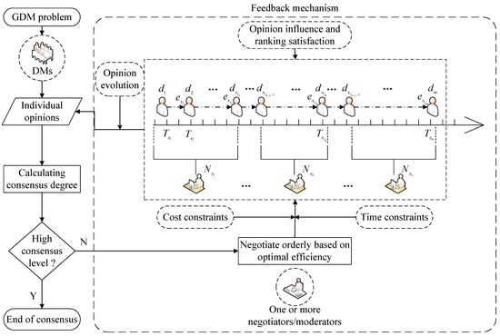
Figure 1.
A framework of sorted cost consensus negotiation.
Decision Variable
Let be a permutation of , representing the sorting sequence of m DMs, i.e.,
- (1)
- For any , .
- (2)
- For any , , .
Definition 1.
Opinion influence level.
The Snajzd model suggests that groups with similar opinions influence the opinion followers around the DMs in these groups to make the same choices as they do [11,12]. When opinions are represented as continuous like interval type, it is impossible to strictly distinguish identical or different opinions and so the level of similarity between opinions can be measured by the opinion similarity.
The BC model reflects the fact that in a social network, when a certain similarity is met between two individuals’ opinions, they are more willing to interact with each other, resulting in the mutual influence and evolution of opinions.
There have been many studies on opinion similarity measures [52], mainly including fuzzy similarity and interval similarity etc. In this paper, the main reference for the similarity measure of interval-type opinions is the Jaccard similarity coefficient [53].
where denotes the Jaccard similarity coefficient of any two sets A and B. The larger the value of , the more similar the sets A and B are.
In the sorted negotiation sequence proposed in this paper, the opinion influence between DMs is unidirectional, as the DM in front influences the DM in back. Therefore, unlike the definition of Jaccard similarity coefficient which is relative to both sets A and B, we aim to measure the opinion influence level of the DM in front relative to the DM in back. Based on this, opinion influence level is used to measure the extent to which opinions of m DMs are affected in the sorting sequence. The formula for the opinion influence level of the individual in ith () position of the sequence is as below:
where denotes the opinion influence level of individual from individual , is overlap length of interval opinions between adjacent individuals and measuring the similarity of opinions between two individuals, is length of the opinion interval of , , where , are the upper and lower bounds of interval respectively. It is clear that .
The extent to which DMs opinions are influenced is related to the overlap length of interval opinions between two adjacent individuals, namely, the higher the relative opinion similarity of two neighboring individuals, the greater the extent to which the opinion of the DM in front influences the DM in back.
The formation of promotive social relationships is primarily determined by opinion similarity [54]; and a basic premise in negotiation research is that individuals sharing similar opinions will improve negotiation processes and outcomes [55,56,57]. Based on these two experimental findings, it can be shown that the higher the overall opinion influence level in the sorted negotiation proposed in our paper, the more it can improve negotiation outcomes and contribute to the sorted consensus negotiations.
Definition 2.
Ranking satisfaction level.
In service industries, waiting due to queuing is a ubiquitous phenomenon, and the ability to manage the queuing and waiting processes scientifically directly determines whether the service recipients are satisfied, while customer satisfaction with the service directly determines whether the enterprise can succeed or fail in its operation. Existing studies show that improving competitiveness in terms of service quality is a key objective for many enterprises [58,59,60]. In this paper, we proposed the sorted consensus negotiation, which is essentially a queuing/scheduling problem, where the DMs are equivalent to the machine parts or the the customers in the queue, and different positions in the negotiation sequence imply different waiting times for DMs. The larger value of i, i.e., the further the position of individual away from the fronter in the sorted negotiation sequence, the longer the negotiation waiting time, and the lower the subjective psychological satisfaction of DM, the more likely the DM will be uncooperative in adjusting to consensus.
The DMs at position i has a negative correlation with his or her subjective psychological satisfaction, namely, the satisfaction level of in negotiation process decreases as his/her position goes back in the sequence; at the same time, we set the ranking satisfaction level of a DM in the interval . Based on the above two points, the formula for ranking satisfaction level is defined as follows:
where is satisfaction level of ith () position and i is the position in which the individual is located. Clearly, .
The ranking satisfaction level estimates the impact of different positions on the sorted negotiation process. In line with Equation , it is conspicuous that the smaller value of i, i.e., closer of the position of individual to the fronter implies higher ranking satisfaction level for him. When the satisfaction levels of DMs are higher, their willingness to cooperate with the moderator in adjusting their opinions is stronger, which in turn contributes to consensus negotiations.
Definition 3.
Opinion order efficiency.
Opinion order efficiency is used to comprehensively measure the effect of opinion influence in different sorting sequences of negotiation, as a function of both opinion influence level and ranking satisfaction level. The formula for opinion order efficiency of is described as follows:
where represents the opinion order efficiency of DM , is opinion influence level of , and is ranking satisfaction level in ith () position of . Since , .
The overall opinion order efficiency is shown as:
where e is the overall opinion order efficiency, namely the sum of opinion order efficiencies of all individuals .
Opinion order efficiency incorporates the effect of opinion influence between similar individuals in the sorted negotiation process and the impact of different positions on the negotiation, merging multiple factors to provide exhaustive measurement toward the sorted negotiation. Equation shows that higher opinion influence level of from the DM in front means higher his opinion order efficiency , and closer to the fronter position implies higher ranking satisfaction level and higher opinion order efficiency .
Definition 4.
Negotiation cost and cost coefficient.
Cost should be taken into account when moderators negotiate with each individual in turn using the sorted negotiation. In GDM, the moderator has to pay a certain amount as compensation to DMs by asking DMs to adjust their opinions, and the compensation is in proportion to the opinion deviation for which the adjustment is made.
Let denote the consensus opinion, represent the opinion of individual , where , is a uniformly distributed random variable. is the unit cost of opinion adjustment towards , and the total cost of opinion adjustments regarding individual is as below:
The total cost of CRP C is the sum of cost of all individuals on opinion adjustments:
In the sorted negotiation, the effect of opinion influence among DMs and ranking in the sorting process are also considered to indirectly affect the unit cost of DM . Specifically, if the higher the opinion order efficiency of a DM, the less difficult it is for the moderator to convince the DM to adjust his or her opinion (the stronger the DM’s willingness to cooperate with the moderator in adjusting his or her opinion), and thus the smaller the unit cost of adjusting the DM’s opinion. In order to abstractly quantify the impact of a DM participating in the sorted negotiation on his or her unit cost , a cost coefficient based on sorted negotiation efficiency is introduced here:
where denotes the cost coefficient of based on opinion order efficiency, is the opinion order efficiency of and the value of is extremely small (e.g., ). Here, is introduced to avoid the cost coefficient . Since , .
With the introduction of a cost coefficient, and assuming for the simplicity of the subsequent calculation process that there is a basic linear relationship between the unit cost of a DM after being affected by the sorted negotiation and his or her original unit cost, the total cost of individual on opinion adjustment becomes , where
The total cost of CRP C becomes , where
After introducing the cost coefficient, it can be seen that the higher opinion order efficiency of , the smaller cost coefficient, indicating that the cost of individual with high opinion order efficiency is cut down, and vice versa. When , the cost coefficient , which means that unit cost is immensely reduced for the current sorting sequence.
Definition 5.
The optimum set of influential individuals and position assessment criteria.
In order to validate the reasonableness of the sorting sequence, i.e., to verify that the DM’s opinion may be influenced by the DM in front, the optimum set of influential individuals is proposed and position assessment criteria are produced. In this paper, we assume that the influence degree of a DM in front on the opinion of a DM in back is related to the similarity of their opinions, namely, the higher opinion similarity between individuals, the higher influence degree. The opinion similarity between DMs is described as follows:
where represents the opinion similarity of individual relative to , denotes overlap length of interval opinions between and , is length of the opinion interval of , and obviously, .
Furthermore, the opinion similarity matrix of all individuals can be obtained:
Concerning the individual , the set consisting of the top among individuals with the greatest opinion similarities (nonzero) with is defined as the optimum set of influential individuals . If only the first individual with the greatest opinion similarity (nonzero) is taken into the set, when an individual is mighty impactive, he/she may be the only person in more than one individual’s sets at the same time. In the sorting sequence, however, it is impossible that an individual is in the position adjacent to more than two individuals simultaneously. It is in reason to take the top t individuals with the greatest opinion similarities (non-zero) with to meet actual situations of sorting problems. The basis for setting is the three levels of general evaluation, namely, good, medium, and poor. Thus the total is divided equally into three. It can be adapted to the needs of different real-life negotiation problems by choosing more detailed and complex classification rules.
On the basis of above, the position assessment criteria is described as follows: In a sorting sequence, an individual satisfies at least one of the four conditions i.e., (1) ; (2) ; (3) ; (4) .
Then, we can conclude that the position of met with the position assessment criteria is considered reasonable and valid, which means that the DM’s position is in front of or behind the positions of DMs with similar opinions to the DM. A sorting sequence is sorted with reason if and only if positions of more than a majority (e.g., 80%) of individuals in the sequence are met with the assessment criteria. For instance, if a sorting sequence is shown in Figure 2, and it is known that , and , then the sequence is considered reasonable in the light of above assessment criteria (Figure 2).
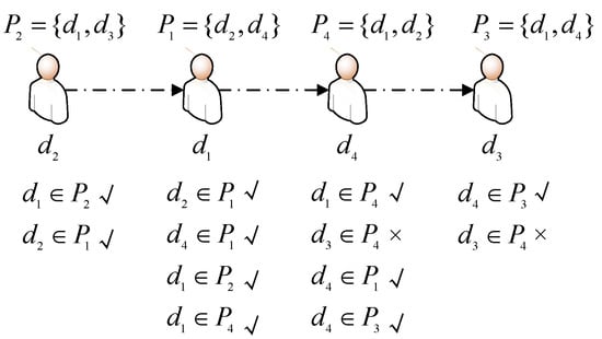
Figure 2.
An example of sequence assessment.
4. The Sorted Negotiation Model Based on Optimal Efficiency
4.1. Basic Assumptions about the Sorting Principles of Group Negotiation
In the sorting sequence of group negotiation, the basic assumptions of sorted negotiation presented in this section are as follows.
Assumption 1.
The influence degree of a DM in front on the opinion of a DM in back is related to the similarity of their opinions, namely, the higher opinion similarity between individuals, the higher influence degree.
Assumption 2.
Compared with the individuals in further positions to the fronter, the individuals in closer positions to the fronter of the sequence are more likely to change their initial opinions, and there is less difficulty in negotiating with them, therefore their opinion order efficiency is relatively high. The opinion order efficiency of the top individual is 1 by default.
4.2. Construction of the Optimal Efficiency Sorted Negotiation Models
The primary intent of this section is to obtain the optimal sorting sequence in which the negotiation is carried out with the highest overall opinion order efficiency, subject to negotiation cost constraints. In the circumstances where the probabilities of the negotiation cost constraints holding are determined, the sorted negotiation Model (19) based on optimal efficiency with chance-constrained programming is developed as follows:
In Model (19), the objective function is the overall opinion order efficiency expected to be maximized of GDM, which is the sum of opinion order efficiency of all individuals . Constraints (19a) and (19b) denote uncertain chance constraints regarding the negotiation cost, indicating probability that negotiation cost does not exceed the budget or is at least p. Constraint (19c) means opinions of DMs obeying uniform distributions. Equation (19d) represents the opinion order efficiency. Equation (19e) and (19f) represent opinion influence level and ranking satisfaction level, respectively. Equationn (19g) describes non-negative constraints on . The known parameters of Model (19) include: , and the parameter is calculated in two cases (as all subsequent models): as a crisp number and as obeying a certain distribution, where the parameters of the distribution are also known.
For the constraints (19a)–(19f) in Model (19), we distinguish two sets of constraints:
- Uncertain chance constraints regarding the negotiation costs,
- Constraints related to the opinion order efficiency,
In the above model, if the probabilities of carrying out negotiation within cost constraints are unknown; then, we expect that the optimal sequence with high opinion order efficiency and negotiation cost constraints satisfied, and the probabilities of accomplishing these goals can be obtained at the same time. In this case, the sorted negotiation Model (20) based on optimal efficiency with chance-constrained programming is constructed as follows:
In Model (20), the objective function expected to be maximized is the overall opinion order efficiency of GDM and the sum of confidence levels related to costs, where a is the equilibrium coefficient, depending on the number of decision individuals and overall efficiency regarding the specific problem. Constraints (20a) and (20b) show uncertain chance constraints regarding the negotiation cost, indicating probability that negotiation cost does not exceed the budget or is at least or . Constraint (20c), (20d) has the same meaning as constraint (19c), (19g), respectively. The known parameters of Model (20) include: .
For the two models above, we assume that the total negotiation cost is deterministic. It is expected not only that the optimal sequence of negotiation is obtained but also that the negotiation cost is as low as possible. The sorted negotiation Model (21) based on optimal efficiency and minimum cost with chance-constrained programming is constructed as follows:
In Model (21), the objective function is the overall opinion order efficiency expected to be maximized of GDM and the total negotiation cost supposed to be minimized, where Q is the equilibrium coefficient, the value of which depends on the specific problem. The known parameters of Model (21) include: .
5. The Optimal Efficiency Sorted Negotiation Model Considering Multi-Moderators Participation and Negotiation Time Constraints
The sorted consensus negotiation is more complex than traditional consensus negotiation, and most notably, it can take more time. Hence, in order to measure the time spent on the sorted negotiation or to cater for time-bound consensus negotiation, we consider the time cost of the sorted negotiation consumption, and the participation of multimoderators can help speed up the process of group negotiation. The optimal efficiency sorted negotiation models are developed that take multimoderators participation and time constraints into account in this paper.
As for a sorted negotiation problem with multimoderators, different moderators take unequal time to negotiate with different individuals, and it is expected that the optimal opinion order efficiency, the optimal sequence of all DMs, the optimal sequence of moderators negotiating and the appropriate amount of DMs assigned to each moderator are obtained with negotiation cost constraints and time constraints satisfying.
5.1. Basic Assumptions
Concerning the group negotiation with multimoderators participation and negotiation time constraints, the basic assumptions about the sorting principles are as follows.
Assumptions 1–2: The same as Assumptions 1–2 in Section 4.1.
Assumption 3.
Each DM is negotiated only once by one moderator, and each moderator can only negotiate with one DM at a time.
5.2. Decision Variable
The supplements to decision variables based on the modeling in Section 3 are as below.
is used to denote the sorting sequence of m decision individuals, where is a positive integer and is a rearrangement (permutation) of the sequence .
is used to denote the sorting sequence of moderators, where is a positive integer and is a rearrangement (permutation) of the sequence satisfying:
- (1)
- For any , .
- (2)
- For any , .
is used to denote the sorted negotiation progress of each moderator corresponding to , which is an integer decision variable satisfying , and where are positive integers indicating the amount of individuals who have completed negotiations as of the moderator .
For any , if , the moderator is not selected for the negotiation.
For any , if , select the moderator for negotiating with in order.
If are given, the corresponding sorting sequence is as shown in Table 1.

Table 1.
The relationship of sorting sequence about moderators and DMs.
For example, when , meaning that there are 8 DMs and 3 moderators involved in a sorted consensus negotiation. If it is known that , then this sorted negotiation is shown in Figure 3.
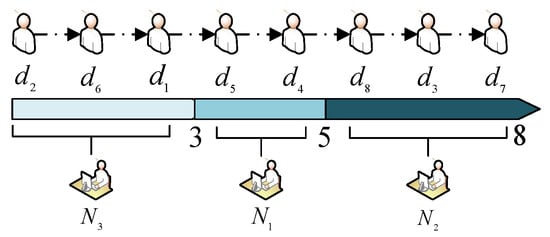
Figure 3.
An example of sorted negotiation.
The sorted negotiation proposed in this manuscript are for all the DMs assigned to different moderator groups and involves negotiating between the moderators and the DMs with no direct negotiation or communication among the DMs. Although the DMs parties belong to different groups of moderators, the negotiation process is a sorted and continuous process within the groups, in which all relevant information for GDM is also fully communicated.
5.3. Description of Negotiation Time
Let represent the time regarding the individual to complete the negotiation, and by induction, it follows that:
where denotes the time regarding the individual to complete the negotiation. represents the time for the moderator negotiating with the individual , and . stands for the time taken for the mth (the last) individual to complete the negotiation, namely, the time taken for the overall negotiation.
5.4. Construction of the Optimal Efficiency Sorted Negotiation Models Considering Multimoderators Participation and Negotiation Time Constraints
The main intent of this section is to obtain the optimal sorting sequence in which the negotiation is carried out with the highest overall efficiency as well as negotiation cost and time constraints satisfying. The optimal efficiency sorted negotiation Model (24) considering multimoderators participation and negotiation time constraints with chance-constrained programming is developed as below, where the probabilities of the negotiation cost and time constraints holding are determined:
In Model (24), the objective function is the overall opinion order efficiency expected to be maximized, which is the sum of the opinion order efficiency of all individuals . Constraints (24a) and (24b) represent uncertain chance constraints with regard to the negotiation completion time, implying probability that negotiation completion time does not exceed the time upper limit or T is at least q. Constraint (24c) describes the inductive relation respecting the negotiation completion time for individual . Constraint (24d) means the negotiation time obeying normal distributions. The known parameters of Model (24) include: .
For the constraints (24a)–(24d) in Model (24), the set of constraints related to the negotiation completion time is summarized:
Similar to Model (20), an optimal efficiency sorted negotiation Model (25) considering multimoderators participation and negotiation time constraints with chance-constrainted programming is constructed as below, where the probabilities of the negotiation cost constraints holding are unknown:
In Model (25), the objective function expected to be maximized is overall opinion order efficiency of GDM and the sum of confidence levels related to costs, where a is the equilibrium coefficient, depending on the amount of decision individuals and overall efficiency regarding the specific problem. Constraints (25a)–(25c) are identical to constraints (20a) and (20c). Equation (25d) describes non-negative constraints on . The known parameters of Model (25) include: .
Similar to Model (21), an optimal efficiency sorted negotiation Model (26) considering multi-moderators participation and negotiation time constraints with chance-constrainted programming is developed as below under the premise that the negotiation budget limit is unknown and desired to be as lower as possible:
In Model (26), the objective function is the overall opinion order efficiency expected to be maximized of GDM and the total negotiation cost supposed to be minimized, where Q is the equilibrium coefficient, the value of which depends on the specific problem. The known parameters of Model (26) include: .
In Models (24)–(26), we assume that the upper limit of negotiation time is deterministic. However, in sorted negotiation with multimoderators participation, it is desired that not only the optimal sequence of negotiation is obtained but also the total negotiation time is as less as possible. To this end, an optimal efficiency sorted negotiation Model (27) considering multimoderators participation and time constraints with chance-constrained programming is constructed as follows:
In Model (27), the objective function is the overall opinion order efficiency expected to be maximized of GDM and the total negotiation time desired to be minimized, where Q is the equilibrium coefficient, the value of which depends on the specific problem. The known parameters of Model (27) include: .
5.5. Improved Genetic Algorithm to Solve Models
A genetic algorithm is a modern optimization algorithm that searches for the optimal solution by simulating the Darwinian biological evolution process. The solution sets of problems to be solved are treated as initial populations, each of which is composed of several individuals considered to be chromosomes. The genetic algorithm means the iteration process where the optimal solution is picked through selection, crossover, and mutation on chromosomes. About the negotiation strategy problem in this paper, decision variables in the feasible set are counted as chromosomes, where are genes that make up the chromosomes. A number of chromosomes are generated randomly during initialization, where integer is used to represent the amount of chromosomes in the population. Improved approaches of the subsequent crossover and mutation on chromosomes are also used to compute the sorted negotiation strategy.
The decision variables are made up of after the introduction of multimoderators and negotiation time, and the algorithm to solve models in Section 4, which is a simplification of the following, is not listed here. The detailed procedures of the improved algorithm are detailed as follows:
- (i)
- The initial is generated randomly. First, define , and . Then repeat the following steps from .
- (a)
- Generate a random integer between j and m.
- (b)
- Swap with .
Up to now, a rearrangement sequence of , namely an initial chromosome, is generated randomly. The decision variable is initialized on the same principle as . For the decision variable , repeat the following steps from .Generate an integer between 0 and m randomly that is assigned to . Then, the initialized sorted by ascending is generated randomly.The generated randomly are integrated as , namely, the initial chromosomes are produced. chromosomes , as the initial population, are generated randomly through repeating the above steps, where . - (ii)
- Suppose ) corresponds to an objective function value , and compute according to the objective function formula in models. Define the evaluation function as .
- (iii)
- Carry out the following selection steps.
- (a)
- The elite chromosome is retained according to the objective function value .
- (b)
- For each , calculate the cumulative probability ..
- (c)
- Generate a random number r from the interval .
- (d)
- If the condition is satisfied, select chromosomes .
- (e)
- Repeat Steps (c) and (d) until replicated chromosomes are obtained.
- (iv)
- Operate crossover on chromosomes . Define as the cross-over probability. First retain the elite chromosome, then repeat the following steps from .
- (a)
- Generate a random number r in the interval .
- (b)
- If , select chromosome as a crossover parent.
The selected chromosomes are paired in sequence, and the following crossover operations are performed on each pair of chromosomes.The paired chromosomes are in the order . For instance, a pair of chromosomes to be crossed is , where let be and operate crossover on the first half genes of in a reference chromosome selected randomly. If the chromosome is chosen as the reference chromosome, traverse externally the first half genes of and traverse internally all the genes of , before recording the positions of the first half genes of in each separately and then moving the corresponding genes to their corresponding positions in line with the recorded positions of the other. The pair becomes . Perform global crossover operations on and the final child chromosomes after the crossover operations are , . Finally, all parent chromosomes are replaced in order with child chromosomes. - (v)
- Operate mutation on chromosomes . Define as the mutation probability. First, retain the elite chromosome, then repeat the following steps from .
- (a)
- Generate a random number r in the interval .
- (b)
- If , select chromosome as a mutation parent.
The selected parent chromosomes to mutate are noted as , . For the chromosome , suppose and perform the following mutation operations on .- (a)
- Generate two random integers .
- (b)
- Let the mutated , where the new subsequence defined as is a rearrangement sequence of the original sequence .
Here, no mutation is performed on . For , operate the following steps of mutation.- (a)
- Generate two random integers .
- (b)
- Let the mutated be , where the new subsequence defined as satisfies by .
The mutated child chromosomes are noted as . Perform the same mutation operations on the other parent chromosomes and the parent chromosomes are replaced with mutated child chromosomes . - (vi)
- Iterate times for Steps (ii) to (v) (e.g., ).
- (vii)
- Return the optimal chromosome representing the optimal decision variable with the optimal objective function value .
Algorithm 1 sets out the procedures for solving Model (24).
| Algorithm 1 Algorithm to solve sorted negotiation model. |
Input:, , , , T, p, q, Output: Sorting sequence and , the negotiation progress of each moderator , total opinion order efficiency e, opinion order efficiency of each individual
|
6. Numerical Example
In order to expound and verify the realistic feasibility of the optimal efficiency sorted negotiation models proposed in Section 4 and Section 5, an numerical example is presented in the context of China’s urban demolition negotiation. House demolition is one of the significant issues about the reform and development of China’s urbanization, which mainly involves negotiations regarding compensation between the Government and relocated residents. The example of China’s urban housing demolition in this paper leans more toward the simplified assumption where external business estate estimates would not significantly differ among the groups of owners, as such housing demolition negotiations in the same area are common in China and valuations of these houses are usually close. In the negotiation process, the Government as the moderator adopts compensation measures to encourage and persuade residents as DMs to move with the ultimate aim of negotiating where the satisfactory amount of compensation for the residents is obtained, and the demolition plan of the Government is completed. In circumstances where multiple government departments are assigned to negotiate with residents on demolition, there are differences in the negotiation completion time among different government departments for different residents, which is owing to differences in skills of leadership, communication among departments. The following issues are addressed in this paper with regard to urban demolition negotiations.
- On the premise of the Government’s budget constraints and negotiation time constraints satisfying, how to complete sorted demolition negotiation with optimal opinion order efficiency.
- On the premise of the Government’s budget constraints and negotiation time constraints satisfying, how to complete sorted demolition negotiation with confidence level and opinion order efficiency as higher as possible.
- On the premise of negotiation time constraints satisfying, how to complete sorted demolition negotiation with lower costs and higher opinion order efficiency.
- On the premise of the Government’s budget constraints satisfying, how to complete sorted demolition negotiation with less time and higher opinion order efficiency.
Suppose that 15 groups of decision residents (i.e., ) are involved in a sorted negotiation process of urban demolition. The initial parameters regarding all resident groups are shown in Table 2, where the opinion interval for each group of decision residents is the more universal one of all data randomly generated from the interval . are, in order, expected compensation amount, unit communication cost, and the Government communication budget of residents .
Table 2.
Data of 15 decision resident groups in urban demolition negotiation.
The parameters of the genetic algorithm are set as , crossover probability , mutation probability , and iteration number . The equilibrium coefficients of models are set to . The process of setting the values of a and Q is as follows: taking Model (20) as an example, we first assign an arbitrary value to a, and then the values of and are all printed out during the solving process. Finally, we observe that the value of is roughly in the interval and the value of is roughly in the interval . So we set , namely reducing in the objective, so that the two items and are basically at the same level of magnitude. Similarly, in Model (21), for example, we can roughly determine that the value of B is roughly in the interval . The idea of this approach is similar to converting a multi-objective programming problem into a single-objective programming problem [61], where each objective is normalized due to the different magnitudes of multiple objectives.
The analysis in this section mainly focuses on the Model (24). The validity of the model is verified in more detail by obtaining the optimal solution through the proposed algorithm and performing sensitivity analysis. All models developed in this paper are based on both cases where the group consensus opinion is known ( is a crisp number) and unknown ( obeys a random distribution), and solutions of models are also presented with two cases in the numerical example that follows. Solutions of the other models in this paper (i.e., Models (19)–(21), Models (25)–(27).) are detailed in Appendix A Table A3, Table A4, Table A5, Table A6, Table A7, Table A8, Table A9 and Table A10.
6.1. Analysis of the Optimal Efficiency Sorted Negotiation Models Considering Multimoderators Participation and Negotiation Time
Based on Models (19)–(21), negotiation time of the government department (moderator) to the resident group (DM) (, .) is introduced into the optimal efficiency sorted negotiation models considering multimoderators participation and negotiation time constraints, which is shown in Table 3.
Table 3.
, .
Case 1: When the group consensus opinion is known (), say the planned compensation of the Government is known to be million, a model based on Model (24) is developed in view of the data of resident groups (DMs) in Table 2 and Table 3 as presented in Appendix A.2, where uncertain chance constraints on negotiation costs (Equations (24a) and (24b)) are computed using stochastic simulations, and uncertain chance constraints on negotiation time (Equations (24c) and (24d)) are calculated by its explicit equivalent constraints to which the cumulative distribution functions of negotiation time () are converted.
Case 2: When the group consensus opinion is unknown (), according to the data in Table 3 and Table 4, the constructed model based on Model (24) is not listed here, where there is no differences from the model in Case 1 of this section except constraints of () and parameters .
Table 4.
Solutions of sorted negotiation model with constraints of both time and cost .
When , solutions of the sorted negotiation model with constraints of both time and cost based on Case 1 (), Case 2 () are shown in Table 4. Taking the solution of Case 1 as an example, the solution shows that the optimal total opinion order efficiency is and the total negotiation time spent is with the budget and the upper limit of overall decision negotiation time . The moderators are required to negotiate with each DM in the sorting sequence . The moderator is responsible for negotiating with the first 10 DMs in the sequence, the moderator is responsible for negotiating with the next 5 DMs in the sequence, and the moderator is not involved in this negotiation. The opinion order efficiency of this sorted negotiation achieved for each DM in the sequence is in order: . The abscissa of the graph denotes the optimal sorting sequence, the ordinate represents DMs’ opinions, and the shaded areas indirectly represent the direction and opinions influence degree among individuals.
In line with Equations (17) and (18) and the initial data of resident groups in Table 2, the opinion similarity matrix among resident groups is obtained:
The optimum sets of influential individuals towards 15 resident groups are obtained according to the top five with the greatest opinion similarities for each group and shown in Table 5.
Table 5.
The optimum sets of Influential Individuals for 15 Resident Groups.
Taking the optimal sorting sequence of Case 1 in Table 4 as an example, it is known according to the position assessment criteria in Definition 5 that of resident groups are in proper positions, which implies that the result of the whole sorting is also efficacious. In the sequence, the residents group in an unreasonable position is , which can be analyzed: Reasons are their last position and extreme opinion. Therefore, in actual negotiation, if the residents cannot be persuaded to adjust their opinions through sorted negotiation even if they are in the last position, management approaches of noncooperative behaviors such as persuading non-cooperative DMs to adjust their opinions and giving them money or other compensation can be adopted. Similarly, the optimal sorting sequence of Case 2 in Table 4 is assessed as reasonable for all resident groups.
When , solutions of the sorted negotiation model with different confidence levels are shown in Appendix Table A1 and Table A2. The results of the sensitivity test for Table A1 and Table A2 are shown in Figure 4.
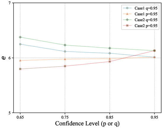
Figure 4.
Sensitivity test on Model (24).
The results of the sensitivity test (Figure 4) reveal that when the budget and the time upper limit T of demolition negotiation given and q unchanged, the lower confidence level p becomes, the higher opinion order efficiency e, which is the broadened restrictions on the cost that make the overall opinion order efficiency increase. If p remains unchanged, as the confidence level q becomes lower, the constraints of negotiation time are broadened and this leads to the negotiation completion time tending to increase. Since confidence level q restricts the negotiation time, it mainly affects the sorting sequence of government departments negotiating and the number of individuals assigned to departments. Still, it does not directly affect the cost and efficiency of sorted negotiation.
In the realistic negotiation of urban demolition and resettlement, the optimal sequencing strategy with optimum opinion order efficiency can be obtained through sorted negotiation models proposed in this paper, where the budget and negotiation completion deadline are learned from the Government. Furthermore, negotiation expenditure of the Government is decreased dramatically, and anticipated outcomes of demolition negotiation are achieved rapidly by means of adopting the reasonable sequencing strategy.
6.2. Analysis of the Algorithm Effectiveness
In order to verify the effectiveness of the genetic algorithm (GA) designed in this paper for solving sorted cost consensus negotiation models, the GA is compared with two algorithms, the artificial bee colony algorithm (ABC) and the simulated annealing algorithm (SAA). ABC is an optimization algorithm proposed to imitate the behaviour of bees, which performs both global and local optimal solution searching during each iteration. However, GA has better global searching capability than ABC since GA includes crossover and mutation operations. SAA derived from the solid annealing principle is a probability-based algorithm that obtains the optimal solution asymptotically by decreasing the temperature. SAA uses single-individual evolution and GA uses population evolution making the algorithm parallel. Since no research has been conducted on the problem of sorted cost consensus negotiation, the above two algorithms are suitably modified to make them applicable to sorted negotiation models when conducting the comparison experiments. To ensure the fairness in experiments, the relevant parameters of the algorithms in the comparison experiments are set as follows: the population size in GA and ABC, the length of Markov chain in SAA, the maximum number of iterations . The experiments were conducted against a model (Case 1: ) based on Model (24). The comparison results are shown in Table 6 and Figure 5, where Best, Mean, Std, and Percent represent the optimum, mean, standard deviation, and proportion of feasible solutions obtained by the algorithm in the process of searching for the optimum, respectively.
Table 6.
Comparative results of GA, ABC and SAA.
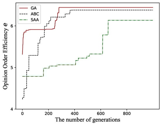
Figure 5.
Convergence curves of GA, ABC and SAA.
It is known from Table 6 that the best and mean by GA on efficiency searching for the sorted cost consensus negotiation model are larger than those of ABC and SAA, and the standard deviations obtained are smaller than those of the other two algorithms. GA generates the highest proportion of feasible solutions in the searching process, which proves that GA has higher searching capability and convergence accuracy, and is also more robust. Figure 5 shows a comparison of the convergence curves of GA, ABC and SAA, from which it is obvious that GA can find the better individual faster and converge with higher accuracy compared to ABC and SAA. The above analysis results show that the GA designed in this paper can effectively solve the sorted cost consensus negotiation models.
7. Conclusions
The theory of opinion dynamics suggests that the opinions of DMs influence each other and further evolve and that the opinions of DMs are more likely to be affected by the opinions of individuals who hold similar ones to their own [49]. In sorted consensus negotiation, the opinion influence of the DM in front on the DM in back in a sequence motivates DMs to adjust their opinions in the direction of similar opinions to those DMs in front. In view of this observation, opinion influence level and ranking satisfaction level are proposed and used to measure the efficiency of opinion order, the cost coefficient is defined to reflect the impact of negotiation sorting on consensus costs, and then optimal efficiency sorted negotiation models are constructed, where the genetic algorithm is adopted to obtain the optimal sorting sequence of DMs. In more intricate GDM, it is also instrumental in upgrading the efficiency of consensus decision making that participation of multiple moderators and restrictions on negotiation time. In the end, the rationality of solutions is confirmed in accordance with defined position assessment criteria in the application example of China’s urban demolition negotiation. The works in this paper are summarized as follows:
- Opinion order efficiency is defined with opinion influence level as well as ranking satisfaction level; furthermore, the optimal efficiency of sorted consensus negotiation is studied for the first time, and the rationality of sorting sequences of optimal efficiency sorted negotiation models is verified by way of introducing an optimum set of influential individuals and position assessment criteria.
- The cost coefficient based on opinion order efficiency is defined, which makes the improvement to cost constraints of sorted negotiation.
- Stochastic distributions (e.g., uniform distributions) are used to fit the uncertainty of DMs’ opinions, and then chance constraints of sorted consensus negotiation costs are developed.
- The uncertainty of negotiation time is described in terms of the time obeying normal distributions for moderator negotiating with individuals, and further optimal efficiency sorted negotiation models considering multi-moderators participation and negotiation time constraints are extended.
Some work can be done in the future:
- The problem of sorted negotiation strategy where opinions of DMs are random variables obeying uniform distributions is investigated in this study. One may conduct a research on sorted negotiation regarding different representation formats of opinions.
- In addition to opinion order efficiency, time, cost of CRP, more factors from multiple aspects may be combined with sorted consensus negotiation, such as characteristics of DMs, social and trust networks in decision groups, multiattributes consensus and clustering for large-scale groups.
- More efficient solving algorithms concerning more complicated sorted negotiation models may be designed.
- Bayesian dynamics can be combined with sorted consensus negotiation.
Author Contributions
Y.Z.: Writing—original draft, Software, Data curation, Formal analysis, Validation, Writing—review and editing, Funding acquisition. C.G.: Conceptualization, Methodology, Supervision, Writing—review and editing, Funding acquisition. G.W.: Formal analysis, Writing—review and editing. E.H.-V.: Supervision, Writing—review and editing, Funding acquisition. All authors have read and agreed to the published version of the manuscript.
Funding
This research was funded by the National Natural Science Foundation of China (grant numbers 71971121), the Major Project Plan of Philosophy and Social Sciences Research at Jiangsu University (grant number 2020SJZDA076), the Jiangsu Postgraduate Research and Practice Innovation Program (grant number 1484052201074).
Data Availability Statement
The data presented in this study are available in insert article.
Conflicts of Interest
The authors declare that there are no conflict of interest.
Appendix A
Appendix A.1. Solutions of Models
Table A1.
Solutions of sorted negotiation model with different p, q (, ).
Table A1.
Solutions of sorted negotiation model with different p, q (, ).
| p | q | e | Total Time | Sorting Sequences and Individual Efficiency |
|---|---|---|---|---|
Table A2.
Solutions of sorted negotiation model with different p, q (, ).
Table A2.
Solutions of sorted negotiation model with different p, q (, ).
| p | q | e | Total Time | Sorting Sequences and Individual Efficiency |
|---|---|---|---|---|
Table A3.
Solutions of sorted negotiation Model (19) for different p (, ).
Table A3.
Solutions of sorted negotiation Model (19) for different p (, ).
| p | e | Sorting Sequences and Individual Efficiency |
|---|---|---|
 | ||
 | ||
 | ||
 | ||
Table A4.
Solutions of sorted negotiation Model (19) for different p (, ).
Table A4.
Solutions of sorted negotiation Model (19) for different p (, ).
| p | e | Sorting Sequences and Individual Efficiency |
|---|---|---|
 | ||
 | ||
 | ||
 | ||
Table A5.
Solutions of sorted negotiation Model (19) .
Table A5.
Solutions of sorted negotiation Model (19) .
| e | Sorting Sequences and Individual Efficiency | ||
|---|---|---|---|
| Case 1 | 2400 | | |
| Case 2 | 4000 | | |
Table A6.
Solutions of sorted negotiation Model (20).
Table A6.
Solutions of sorted negotiation Model (20).
| e | Sorting Sequences and Individual Efficiency | ||||
|---|---|---|---|---|---|
| Case 1 | 2200 | ||||
| Case 2 | 2800 | ||||
Table A7.
Solutions of sorted negotiation Model (21).
Table A7.
Solutions of sorted negotiation Model (21).
| p | e | B | Sorting Sequences and Individual Efficiency | ||
|---|---|---|---|---|---|
| Case 1 | |||||
| Case 2 | |||||
Table A8.
Solutions of sorted negotiation Model (24) ().
Table A8.
Solutions of sorted negotiation Model (24) ().
| e | Time | Sorting Sequences and Individual Efficiency | ||||
|---|---|---|---|---|---|---|
| Case 1 | 2200 | |||||
| Case 2 | 3500 | |||||
Table A9.
Solutions of sorted negotiation Model (25) ().
Table A9.
Solutions of sorted negotiation Model (25) ().
| p | e | B | Time | Sorting Sequences and Individual Efficiency | ||
|---|---|---|---|---|---|---|
| Case 1 | ||||||
| Case 2 | ||||||
Table A10.
Solutions of sorted negotiation Model (26) ().
Table A10.
Solutions of sorted negotiation Model (26) ().
| e | T | Sorting Sequences and Individual Efficiency | |||
|---|---|---|---|---|---|
| Case 1 | 2500 | ||||
| Case 2 | 4100 | ||||
Appendix A.2. The Specific Model in Numerical Example
Appendix A.3. Symbol Description
See Table A11:
Table A11.
Symbol description.
Table A11.
Symbol description.
| Symbol | Description | Type |
|---|---|---|
| The symbol of DM i, . | Symbol | |
| The symbol of moderator k, . | Symbol | |
| The DM in ith position, , where is a rearrangement (permutation) of . | Symbol | |
| The opinion influence level of on , , . | Variable | |
| The ranking satisfaction level of , . | Variable | |
| Overlap length of interval opinions between two adjacent individuals and . | Variable | |
| Overlap length of interval opinions between and . | Parameter | |
| Opinion interval of , where , are the upper and lower bounds of interval respectively. | Parameter | |
| Length of the opinion interval of , . | Parameter | |
| Opinion similarity of individual with respect to . | Parameter | |
| S | Opinion similarity matrix of all DMs. | Parameter |
| The optimum set of influential individuals towards individual . | Symbol | |
| The opinion of , . | Variable | |
| e | Overall opinion order efficiency. | Variable |
| Opinion order efficiency of the , . | Variable | |
| Unit cost of opinion adjustment towards . | Variable | |
| The cost coefficient of based on opinion order efficiency. | Variable | |
| Group consensus opinion. | Parameter | |
| The adjusted opinion of . | Parameter | |
| The opinion of DM in the tth round. | Symbol | |
| The weight that DM gives to at round t. | Parameter | |
| The confidence set of DM . | Symbol | |
| B | Total cost of consensus reaching. | Variable |
| Total budget of consensus reaching. | Parameter | |
| Negotiation cost upper limit of . | Variable | |
| p | Probability/confidence level, . | Parameter |
| Negotiation time of the moderator towards the individual , , . | Parameter | |
| Actual time to accomplish negotiation for . | Variable | |
| Upper limit of negotiation time for . | Parameter | |
| T | Upper limit of overall decision negotiation time. | Parameter |
| q | Probability/confidence level, . | Parameter |
| Q | Larger equilibrium coefficient. | Parameter |
| Smaller equilibrium coefficients. | Parameter | |
| The bounded confidence level. | Parameter | |
| Maximum number of iterations. | Parameter |
Appendix A.4. Algorithm Execute Script
import matplotlib.pyplot as plt
import random
import numpy as np
from scipy.stats import norm
from copy import deepcopy
def init(size):
pop_ = []
dmlst_ = dmlst.copy()
ylst_ = ylst.copy()
for i in range(size) :
xy = []
y_ = []
for j in range(M) :
dmlst_ = dmlst_.copy()
rn_ = random.randint(j, M-1)
dmlst_[j], dmlst_[rn_] = dmlst_[rn_], dmlst_[j]
xy.append(dmlst_)
for k in range(n) :
ylst_ = ylst_.copy()
ry = random.randint(k,n-1)
ylst_[k], ylst_[ry] = ylst_[ry], ylst_[k]
for s in range(n-1) :
rs = random.randint(0,M)
y_.append(rs)
y_.append(M)
y_dict = dict(zip(ylst_, y_))
yy = sorted(y_dict.items(),key=lambda x:x[1],reverse=False)
xy.append(yy)
pop_.append(xy)
return(pop_)
def evaluate(ppop):
pre_evals = []
pre_alpha = []
for i in range(pop_size) :
olst = []
for j in range(M) :
olst.append(dm_dict[ppop[i][0][j]])
esum_ = 1.0
alpha = []
alpha.append( 1.0 )
for k in range(1,M) :
if olst[k-1][1] <= olst[k][0] or olst[k][1] <= olst[k-1][0]:
overl = 0.0001
if olst[k-1][0] < olst[k][0] and olst[k][1] < olst[k-1][1] :
overl = olst[k][1] - olst[k][0]
if olst[k][0] < olst[k-1][0] and olst[k-1][1] < olst[k][1] :
overl = olst[k-1][1] - olst[k-1][0]
if olst[k-1][0] <= olst[k][0] and olst[k][0] < olst[k-1][1] and olst[k-1][1] <= olst[k][1] :
overl = olst[k-1][1] - olst[k][0]
if olst[k][0] <= olst[k-1][0] and olst[k-1][0] < olst[k][1] and olst[k][1] <= olst[k-1][1] :
overl = olst[k][1] - olst[k-1][0]
alpha_i = overl / (olst[k][1] - olst[k][0])
alpha.append(alpha_i)
ek = alpha_i * beta[k]
esum_ += ek
pre_evals.append(esum_)
pre_alpha.append(alpha)
return pre_evals, pre_alpha
def check(pevals, palpha, ppop):
pre_evals = []
pre_alpha = []
pre_pop = []
pre_T = []
while True:
N = 50
for i in range(pop_size):
olst = []
cxi_lst = []
bi_lst = []
for j in range(M) :
olst.append(dm_dict[ppop[i][0][j]])
cxi_lst.append(cxi_dict[ppop[i][0][j]])
bi_lst.append(Bi_dict[ppop[i][0][j]])
fitm = 0
fitn = 0
c1 = []
o_xi = []
for j in range(M) :
c1.append(1 - ( palpha[i][j] * beta[j] ) + epsilon)
o_xi.append(np.random.uniform(olst[j][0], olst[j][1], N))
for j in range(M) :
Pm = 0
for k in range(0,N) :
Bm = ( c1[j] * cxi_lst[j] * abs(o_ - o_xi[j][k]) )
if Bm - bi_lst[j] <= 0 :
Pm += 1
if float(Pm/N) >= p :
fitm += 1
o_i = []
for j in range(0,N) :
_oxi =[]
for k in range(M) :
_oxi.append(o_xi[k][j])
o_i.append(_oxi)
for j in range(N) :
B_sum = 0
for k in range(M) :
B_ = ( c1[k] * cxi_lst[k] * abs(o_ - o_i[j][k]) )
B_sum += B_
if B_sum - B <= 0 :
fitn += 1
if float(fitn/N) >= p and fitm == M :
Xi_ilst = []
for j in range(M) :
no_ = ppop[i][0][j] - 1
if j+1 > 0 and j+1 <= ppop[i][1][0][1] :
ma_no = ppop[i][1][0][0] - 1
Xi_ilst.append( [Xi_mu[no_][ma_no], Xi_sig[no_][ma_no]] )
if j+1 > ppop[i][1][0][1] and j+1 <= ppop[i][1][1][1] :
ma_no = ppop[i][1][1][0] - 1
Xi_ilst.append( [Xi_mu[no_][ma_no], Xi_sig[no_][ma_no]] )
if j+1 > ppop[i][1][1][1] and j+1 <= ppop[i][1][2][1] :
ma_no = ppop[i][1][2][0] - 1
Xi_ilst.append( [Xi_mu[no_][ma_no], Xi_sig[no_][ma_no]] )
T_xia = 0
T_xib = 0
for j in range(M) :
T_xia += Xi_ilst[j][0]
T_xib += Xi_ilst[j][1]
norm_xi = norm(T_xia, T_xib)
fai_ = norm_xi.ppf(alpa)
if j == M-1 :
TT = fai_
if TT <= T_sum :
pre_T.append(TT)
pre_evals.append(deepcopy( pevals[i] ) )
pre_alpha.append(deepcopy( palpha[i][:]) )
pre_pop.append( deepcopy( ppop[i][:][:]) )
if len(pre_pop) < pop_size :
ppop = crossover(ppop[:][:])
ppop = mutate(ppop[:][:])
pevals, palpha = evaluate(ppop)
else :
pre_evals = pre_evals[:pop_size]
pre_alpha = pre_alpha[:pop_size]
pre_pop = pre_pop[:pop_size][:]
break
return pre_evals, pre_alpha, pre_T, pre_pop
def copy(ppop, pevals):
pre_pop = []
pre_pop.append(ppop[pevals.index(max(pevals))])
p = []
p_accumulate = []
for i in range(pop_size):
p.append(1.0 * pevals[i] / sum(pevals))
for i in range(1, pop_size + 1):
p_accumulate.append(sum(p[:i]))
for i in range(pop_size - 1):
r_num = random.random()
for j in range(pop_size - 1):
if r_num < p_accumulate[0]:
pre_pop.append(ppop[0][:])
break
if p_accumulate[j] <= r_num < p_accumulate[j + 1]:
pre_pop.append(ppop[j + 1][:])
break
return pre_pop
def crossover(ppop):
best = ppop[0][:][:]
ppop = ppop[1:][:]
cros_freq = 0
while True:
cros_index = []
for i in range(pop_size - 1):
rand_num = random.random()
if rand_num < cp:
cros_index.append(i)
if len(cros_index) % 2 == 0 and cros_index != []:
break
point_num = int(len(cros_index) / 2)
for i in range(point_num) :
ppop[cros_index[i * 2]][1][:], ppop[cros_index[i * 2 + 1]][1][:] = ppop[cros_index[i * 2 + 1]][1][:], ppop[cros_index[i * 2]][1][:]
for j in range(M) :
for k in range(M) :
if ppop[cros_index[i * 2]][0][j] == ppop[cros_index[i * 2 + 1]][0][k] :
ppop[cros_index[i * 2]][0][j], ppop[cros_index[i * 2]][0][k] = ppop[cros_index[i * 2]][0][k], ppop[cros_index[i * 2]][0][j]
ppop[cros_index[i * 2 + 1]][0][j], ppop[cros_index[i * 2 + 1]][0][k] = ppop[cros_index[i * 2 + 1]][0][k], ppop[cros_index[i * 2 + 1]][0][j]
break
cros_freq += 1
if cros_freq == int(0.5*M) :
break
else :
continue
ppop.insert(0, best)
return ppop
def mutate(ppop):
best = ppop[0][:][:]
ppop = ppop[1:][:]
while True:
mut_index = []
for i in range(pop_size - 1):
r_num = random.random()
if r_num < mp:
mut_index.append(i)
if mut_index != []:
break
for i in range(len(mut_index)):
n1 = random.randint(0, M-1)
n2 = random.randint(0, M-1)
n1, n2 = min(n1, n2), max(n1, n2)
del_num = n2 - n1 + 1
del_freq = 0
newlst = ppop[mut_index[i]][0][n1:n2 + 1]
while del_freq < del_num :
del ppop[mut_index[i]][0][n1]
del_freq += 1
random.shuffle(newlst)
for j in range(len(newlst)) :
ppop[mut_index[i]][0].insert(n1 + j, newlst[j])
if len(ppop[mut_index[i]][0]) == M :
break
for i in range(len(mut_index)):
yyy = []
n5 = random.randint(1, n-2)
n6 = random.randint(1, n-2)
n5, n6 = min(n5, n6), max(n5, n6)
for j in range(n5, n6+1) :
n3 = random.randint(ppop[mut_index[i]][1][n5-1][1], ppop[mut_index[i]][1][n6+1][1])
yyy.append(n3)
yyy.sort()
for j in range(n5, n6+1) :
s = 0
pint = list(ppop[mut_index[i]][1][n5])
pint[1] = yyy[s]
ppop[mut_index[i]][1][n5] = tuple(pint)
s += 1
ppop.insert(0, best)
return ppop
if __name__ == ’__main__’:
References
- Cook, W.D.; Kress, M. Ordinal ranking with intensity of preference. Manag. Sci. 1985, 31, 26–32. [Google Scholar] [CrossRef]
- Hochbaum, D.S.; Levin, A. Methodologies and algorithms for group-rankings decision. Manag. Sci. 2006, 52, 1394–1408. [Google Scholar] [CrossRef]
- Zhang, B.W.; Dong, Y.C.; Zhang, H.J.; Pedrycz, W. Consensus mechanism with maximum-return modifications and minimum-cost feedback: A perspective of game theory. Eur. J. Oper. Res. 2020, 287, 546–559. [Google Scholar] [CrossRef]
- French, J.R.P.J. A formal theory of social power. Psychol. Rev. 1956, 63, 181–194. [Google Scholar] [CrossRef] [PubMed]
- Berger, R.L. A necessary and sufficient condition for reaching a consensus using DeGroot’s method. J. Am. Stat. Assoc. 1981, 76, 415–418. [Google Scholar] [CrossRef]
- Degroot, M.H. Reaching a Consensus. J. Am. Stat. Assoc. 1974, 69, 118–121. [Google Scholar] [CrossRef]
- Friedkin, N.E.; Johnsen, E.C. Social influence and opinions. J. Math. Sociol. 1990, 15, 193–206. [Google Scholar] [CrossRef]
- Pérez, L.; Mata, F.; Chiclana, F.; Kou, G.; Herrera-Viedma, E. Modelling influence in group decision making. Soft Comput.-A Fusion Found. Methodol. Appl. 2016, 20, 1653–1665. [Google Scholar] [CrossRef]
- Deffuant, G.; Neau, D.; Amblard, F.; Weisbuch, G. Mixing beliefs among interacting agents. Adv. Complex Syst. 2000, 3, 87–98. [Google Scholar] [CrossRef]
- Hegselmann, R.; Krause, U. Opinion dynamics and bounded confidence: Models, analysis and simulation. J. Artif. Soc. Soc. Simul. 2002, 5. [Google Scholar]
- Rodrigues, F.A.; Da FCosta, L. Surviving opinions in sznajd models on complex net works. Int. J. Mod. Phys. C Comput. Phys. Phys. Comput. 2015, 16, 1785–1792. [Google Scholar]
- Stauffer, D. Sociophysics: The Sznajd model and its applications. Comput. Phys. Commun. 2002, 146, 93–98. [Google Scholar] [CrossRef]
- Capuano, N.; Chiclana, F.; Fujita, H.; Herrera-Viedma, E.; Loia, V. Fuzzy Group Decision Making With Incomplete Information Guided by Social Influence. IEEE Trans. Fuzzy Syst. 2018, 26, 1704–1718. [Google Scholar] [CrossRef]
- Liu, B.S.; Zhou, Q.; Ding, R.X.; Palomares, I.; Herrera, F. Large-scale group decision making model based on social network analysis: Trust relationship-based conflict detection and elimination. Eur. J. Oper. Res. 2019, 275, 737–754. [Google Scholar] [CrossRef]
- Li, Y.H.; Kou, G.; Li, G.X.; Peng, Y. Consensus reaching process in large-scale group decision making based on bounded confidence and social network. Eur. J. Oper. Res. 2022, 199, 509–516. [Google Scholar] [CrossRef]
- Xu, Y.X.; Gong, Z.W.; Wei, G.; Guo, W.W.; Herrera-Viedma, E. Information consistent degree-based clustering method for large-scale group decision-making with linear uncertainty distributions information. INternational J. Intell. Syst. 2022, 37, 3394–3439. [Google Scholar] [CrossRef]
- Gong, Z.W.; Xu, X.X.; Li, L.S.; Xu, C. Consensus modeling with nonlinear utility and cost constraints: A case study. Knowl.-Based Syst. 2015, 88, 210–222. [Google Scholar] [CrossRef]
- Altuzarra, A.; Moreno-Jiménez, J.M.; Salvador, M. Consensus Building in AHP-Group Decision Making: A Bayesian Approach. Oper. Res. 2010, 58, 1755–1773. [Google Scholar] [CrossRef]
- Gong, Z.W.; Zhang, N.; Chiclana, F. The optimization ordering model for intuitionistic fuzzy preference relations with utility functions. Knowl.-Based Syst. 2018, 162, 174–184. [Google Scholar] [CrossRef]
- Mayag, B.; Bouyssou, D. Necessary and possible interaction between criteria in a 2-additive Choquet integral model. Eur. J. Oper. Res. 2020, 283, 308–320. [Google Scholar] [CrossRef]
- Fishburn, P.C.; Kress, M. Utility Theory for Decision Making; Robert E. Krieger Publishing Company: Malabar, FL, USA, 1979. [Google Scholar]
- Yazidi, A.; Ivanovska, M.; Zennaro, F.M.; Lind, P.G.; Viedma, E.H. A new decision making model based on Rank Centrality for GDM with fuzzy preference relations. Eur. J. Oper. Res. 2022, 297, 1030–1041. [Google Scholar] [CrossRef]
- Marimuthu, D.; Meidute-Kavaliauskiene, I.; Mahapatra, G.S.; Činčikaitė, R.; Roy, P.; Vasiliauskas, A.V. Sustainable Urban Conveyance Selection through MCGDM Using a New Ranking on Generalized Interval Type-2 Trapezoidal Fuzzy Number. Mathematics 2022, 10, 4534. [Google Scholar] [CrossRef]
- Aggarwal, M. Linguistic discriminative aggregation in multicriteria decision making. Int. J. Intell. Syst. 2016, 31, 529–555. [Google Scholar] [CrossRef]
- Gong, Z.W.; Guo, W.W.; Herrera-Viedma, E.; Gong, Z.J.; Wei, G. Consistency and consensus modeling of linear uncertain preference relations. Eur. J. Oper. Res. 2020, 283, 290–307. [Google Scholar] [CrossRef]
- Zhang, N.; Gong, Z.W.; Chiclana, F. Minimum cost consensus models based on random opinions. Expert Syst. Appl. 2017, 89, 149–159. [Google Scholar] [CrossRef]
- Wang, L.Z.; Fang, L.P.; Hipel, K.W. Basin-wide cooperative water resources allocation. Eur. J. Oper. Res. 2008, 190, 798–817. [Google Scholar] [CrossRef]
- Radner, R. Decision and Choice: Bounded Rationality. In International Encyclopedia of the Social & Behavioral Sciences; Pergamon: Oxford, UK, 2015; pp. 879–885. [Google Scholar]
- Simon, H.A. Theories of bounded rationality. Decis. Organ. 1972, 161–176. [Google Scholar]
- Palomares, I.; Martínez, L.; Herrera, F. A Consensus Model to Detect and Manage Noncooperative Behaviors in Large-Scale Group Decision Making. IEEE Trans. Fuzzy Syst. 2014, 22, 516–530. [Google Scholar] [CrossRef]
- Chao, X.R.; Kou, G.; Peng, Y.; Herrera-Viedma, E. Large-scale group decision-making with non-cooperative behaviors and heterogeneous preferences: An application in financial inclusion. Eur. J. Oper. Res. 2021, 288, 271–293. [Google Scholar] [CrossRef]
- Dong, Y.C.; Zhang, H.J.; Herrera-Viedma, E. Integrating experts’ weights generated dynamically into the consensus reaching process and its applications in managing non-cooperative behaviors. Decis. Support Syst. 2016, 84, 1–15. [Google Scholar] [CrossRef]
- Cheng, D.; Yuan, Y.X.; Wu, Y.; Hao, T.T.; Cheng, F.X. Maximum satisfaction consensus with budget constraints considering individual tolerance and compromise limit behaviors. Eur. J. Oper. Res. 2022, 297, 221–238. [Google Scholar] [CrossRef]
- Ben-Arieh, D.; Easton, T. Multi-criteria group consensus under linear cost opinion elasticity. Decis. Support Syst. 2007, 43, 713–721. [Google Scholar] [CrossRef]
- Ben-Arieh, D.; Easton, T.; Evans, B. Minimum Cost Consensus With Quadratic Cost Functions. IEEE Trans. Syst. Man Cybern.-Part A Syst. Hum. 2009, 39, 210–217. [Google Scholar] [CrossRef]
- Dong, Y.C.; Xu, Y.F.; Li, H.Y.; Feng, B. The OWA-based consensus operator under linguistic representation models using position indexes. Eur. J. Oper. Res. 2010, 203, 455–463. [Google Scholar] [CrossRef]
- Zhang, G.Q.; Dong, Y.C.; Xu, Y.F.; Li, H.Y. Minimum-Cost Consensus Models Under Aggregation Operators. IEEE Trans. Syst. Man, Cybern.-Part A Syst. Hum. 2011, 41, 1253–1261. [Google Scholar] [CrossRef]
- Wu, Z.; Zhu, K.; Qu, S. Distributionally Robust Optimization Model for a Minimum Cost Consensus with Asymmetric Adjustment Costs Based on the Wasserstein Metric. Mathematics 2022, 10, 312. [Google Scholar] [CrossRef]
- Gong, Z.W.; Zhang, H.H.; Forrest, J.; Li, L.S.; Xu, X.X. Two consensus models based on the minimum cost and maximum return regarding either all individuals or one individual. Eur. J. Oper. Res. 2015, 240, 183–192. [Google Scholar] [CrossRef]
- Wu, Z.B.; Tu, J.C. Managing transitivity and consistency of preferences in AHP group decision making based on minimum modifications. Inf. Fusion 2021, 67, 125–135. [Google Scholar] [CrossRef]
- Parreiras, R.O.; Ekel, P.Y.; Martini, J.S.C.; Palhares, R.M. A flexible consensus scheme for multicriteria group decision making under linguistic assessments. Inf. Sci. 2010, 180, 1075–1089. [Google Scholar] [CrossRef]
- Zhang, B.W.; Dong, Y.C.; Xu, Y.F. Multiple attribute consensus rules with minimum adjustments to support consensus reaching. Knowl.-Based Syst. 2014, 67, 35–48. [Google Scholar] [CrossRef]
- Zhang, H.J.; Dong, Y.C.; Chiclana, F.; Yu, S. Consensus efficiency in group decision making: A comprehensive comparative study and its optimal design. Eur. J. Oper. Res. 2019, 275, 580–598. [Google Scholar] [CrossRef]
- Wu, Z.B.; Huang, S.; Xu, J.P. Multi-stage optimization models for individual consistency and group consensus with preference relations. Eur. J. Oper. Res. 2019, 275, 182–194. [Google Scholar] [CrossRef]
- Cheng, D.; Zhou, Z.L.; Cheng, F.X.; Zhou, Y.F.; Xie, Y.J. Modeling the minimum cost consensus problem in an asymmetric costs context. Eur. J. Oper. Res. 2018, 270, 1122–1137. [Google Scholar] [CrossRef]
- Gong, Z.W.; Xu, C.; Chiclana, F. Consensus Measure with Multi-stage Fluctuation Utility Based on China’s Urban Demolition Negotiation. Group Decis. Negot. 2017, 26, 379–407. [Google Scholar] [CrossRef]
- Abdel-Basset, M.; Mohamed, R.; Chakrabortty, R.K.; Ryan, M.J. IEGA: An improved elitism-based genetic algorithm for task scheduling problem in fog computing. Int. J. Intell. Syst. 2021, 36, 4592–4631. [Google Scholar] [CrossRef]
- Wan, Q.; Xu, X.; Chen, X. A Two-Stage Optimization Model for Large-Scale Group Decision-Making in Disaster Management: Minimizing Group Conflict and Maximizing Individual Satisfaction. Group Decis. Negot. 2020, 29, 901–921. [Google Scholar] [CrossRef]
- Elgazzar, A.S. Application of the sznajd sociophysics model to small-world networks. Int. J. Mod. Phys. C Comput. Phys. Phys. Comput. 2001, 12, 1537. [Google Scholar] [CrossRef]
- Zha, Q.B.; Kou, G.; Zhang, H.J.; Liang, H.M.; Chen, X.; Li, C.C.; Dong, Y.C. Opinion dynamics in finance and business: A literature review and research opportunities. Financ. Innov. 2022, 6, 1–22. [Google Scholar] [CrossRef]
- Weisbuch, G.; Deffuant, G.; Amblard, F.; Nadal, J.P. Meet, discuss, and segregate! Complexity 2002, 7, 55–63. [Google Scholar] [CrossRef]
- Chiclana, F.; García, J.M.T.; del Moral, M.J.; Herrera-Viedma, E. A statistical comparative study of different similarity measures of consensus in group decision making. Inf. Sci. 2013, 221, 110–123. [Google Scholar] [CrossRef]
- Jaccard, P. The distribution of the flora in the alpine zone. New Phytol. 2010, 11, 37–50. [Google Scholar] [CrossRef]
- Sole, K.; Marton, J.; Hornstein, H.A. Opinion similarity and helping: Three field experiments investigating the bases of promotive tension. J. Exp. Soc. Psychol. 1975, 11, 1–13. [Google Scholar] [CrossRef]
- Ang, S.H.; Leong, S.M.; Teo, G.P. The Effects of Personal Value Similarity on Business Negotiations. Ind. Mark. Manag. 2000, 29, 397–410. [Google Scholar] [CrossRef]
- Campbell, N.; Graham, J.L.; Jolibert, A.; Meissner, H.G. Marketing Negotiations in France, Germany, the United Kingdom, and the United States. J. Mark. 1988, 52, 49. [Google Scholar] [CrossRef]
- Graham, J.L. Cross-Cultural Marketing Negotiations: A Laboratory Experiment. Mark. Sci. 1985, 4, 130–146. [Google Scholar] [CrossRef]
- Allon, G. Competition in Service Industries. Ph.D. Thesis, Columbia University, New York, NY, USA, 2006. [Google Scholar]
- Cachon, G.P.; Harker, P.T. Competition and Outsourcing with Scale Economies. Manag. Sci. 2002, 48, 1314–1333. [Google Scholar] [CrossRef]
- Ho, T.H. Setting Customer Expectation in Service Delivery: An Integrated Marketing-Operations Perspective. Manag. Sci. 2004, 50, 479–488. [Google Scholar] [CrossRef]
- Tamiz, M.; Jones, D.; Romero, C. Goal programming for decision making: An overview of the current state-of-the-art. Eur. J. Oper. Res. 1998, 111, 569–581. [Google Scholar] [CrossRef]


Disclaimer/Publisher’s Note: The statements, opinions and data contained in all publications are solely those of the individual author(s) and contributor(s) and not of MDPI and/or the editor(s). MDPI and/or the editor(s) disclaim responsibility for any injury to people or property resulting from any ideas, methods, instructions or products referred to in the content. |
© 2023 by the authors. Licensee MDPI, Basel, Switzerland. This article is an open access article distributed under the terms and conditions of the Creative Commons Attribution (CC BY) license (https://creativecommons.org/licenses/by/4.0/).