
Sensitivity of Survival Analysis Metrics

Abstract
:1. Introduction
2. Background
2.1. Problem Statement
2.2. Statistical Models
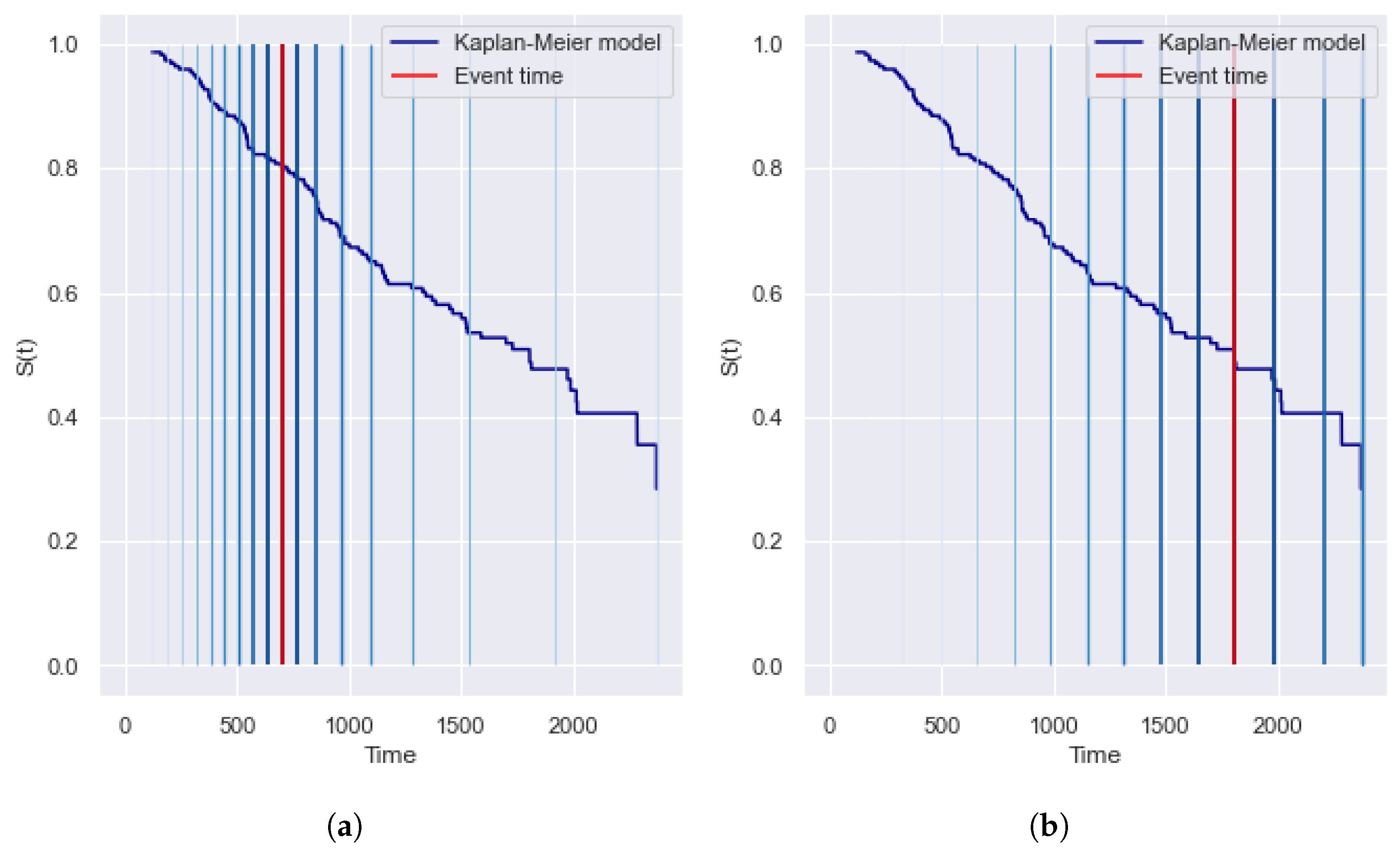
2.2.1. Kaplan–Meier Estimator
2.2.2. Cox Proportional Hazard
- The ratio of two hazard functions does not change over time;
- The significance of features does not depend on time. In real clinical practice, the influence of risk factors may vary over time. For example, the patient is at risk after surgery, but after rehabilitation is more stable;
- The weights of the model define a linear combination of the data features;
- CoxPH does not support categorical features and missing values.
2.3. Metrics
2.3.1. Concordance Index
2.3.2. Integrated AUC
2.3.3. Likelihood
2.3.4. Kullback–Leibler Divergence
2.3.5. Integrated Brier Score
2.3.6. AUPRC
2.3.7. Motivation for Choosing a Metric
- 1.
- metric for estimating the time of the event T. For censored observations, considers only pairs that the second event occurred before the moment of censoring.
- 2.
- metric for estimating the hazard function, . Unlike the metric, evaluates the overall survival function.
- 3.
- and metrics for estimating the survival function, . Unlike , these metrics take into account censored observations. In addition, is limited by the nonparametric survival function, , which does not use the feature space of observations.
2.4. Machine Learning Models
2.4.1. Log-Rank Criterion
- 1.
- Wilcoxon weights are the number of remaining observations at the time.
- 2.
- Peto-peto weights are the value of the parent survival function at the time.
- 3.
- Tarone-ware weights are the square root of the number of observations at the time. Tarone-Ware is the “golden mean” among weighted criteria [1].
2.4.2. Survival Tree
2.4.3. Random Survival Forest
- 1.
- Build N bootstrap samples (with replacement) from the source sample. Each bootstrap subsample excludes approximately 37% of the data, which is called out-of-bag (OOB);
- 2.
- Build a survival tree for each bootstrap sample [22]. Finding the best partition uses only P features at each node. The best partition maximizes the difference between child nodes;
- 3.
- Each survival tree is built until bootstrap sampling is exhausted. In other words, there are no restrictions on the depth and number of observations for trees.
2.4.4. Survival Bagging
2.4.5. Gradient Boosting Survival Analysis
2.4.6. Component-Wise Gradient Boosting
2.5. Summary
3. Methodology
4. Real Data Description
- 1.
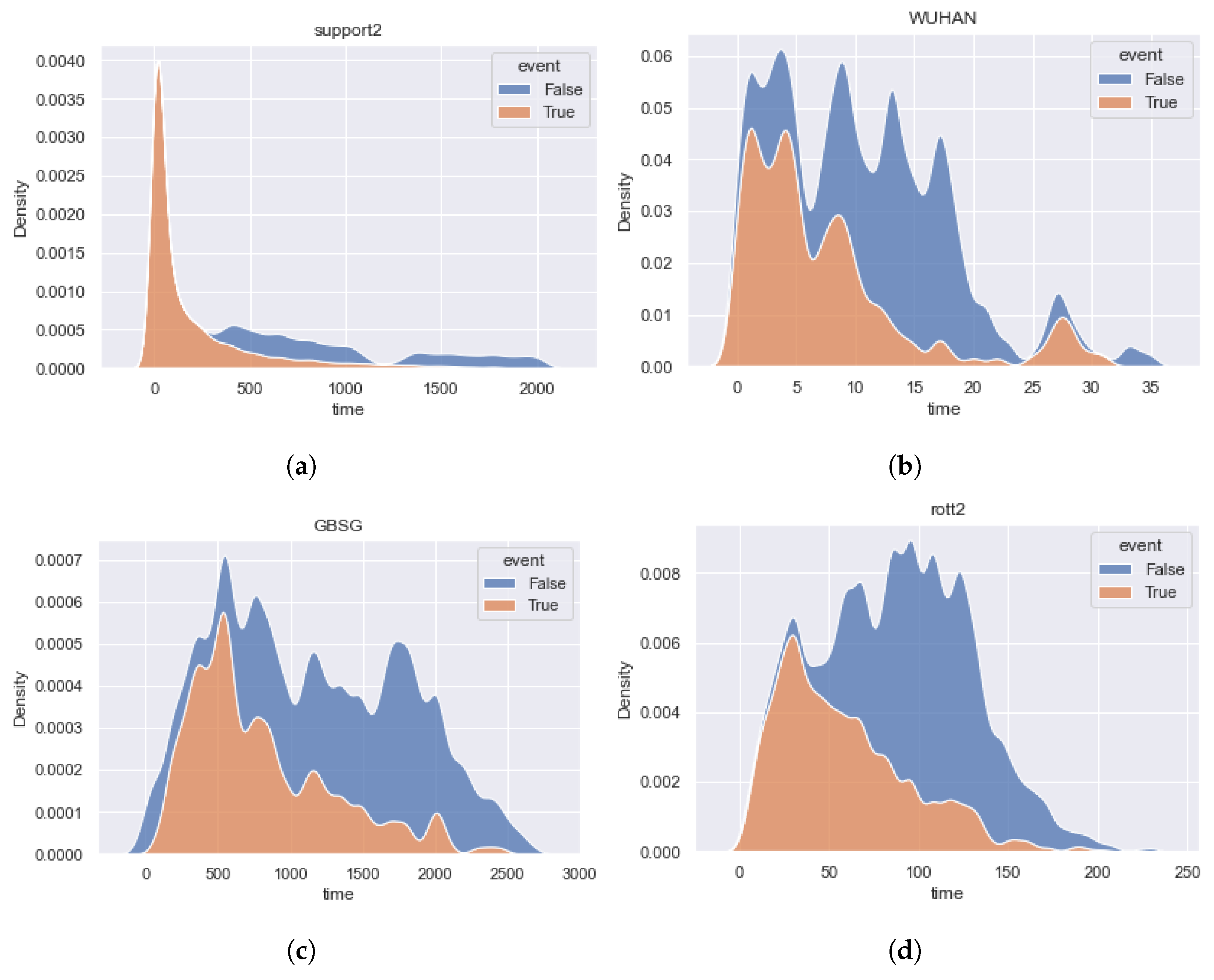
- Early events have the highest significance for the dataset because the data describes the incurable patients using life support devices. The imbalance of event classes is biased toward terminal events.
- 2.
- The , , , and datasets are balanced relative to the event classes, and the early and middle events have the greatest importance.
- 3.
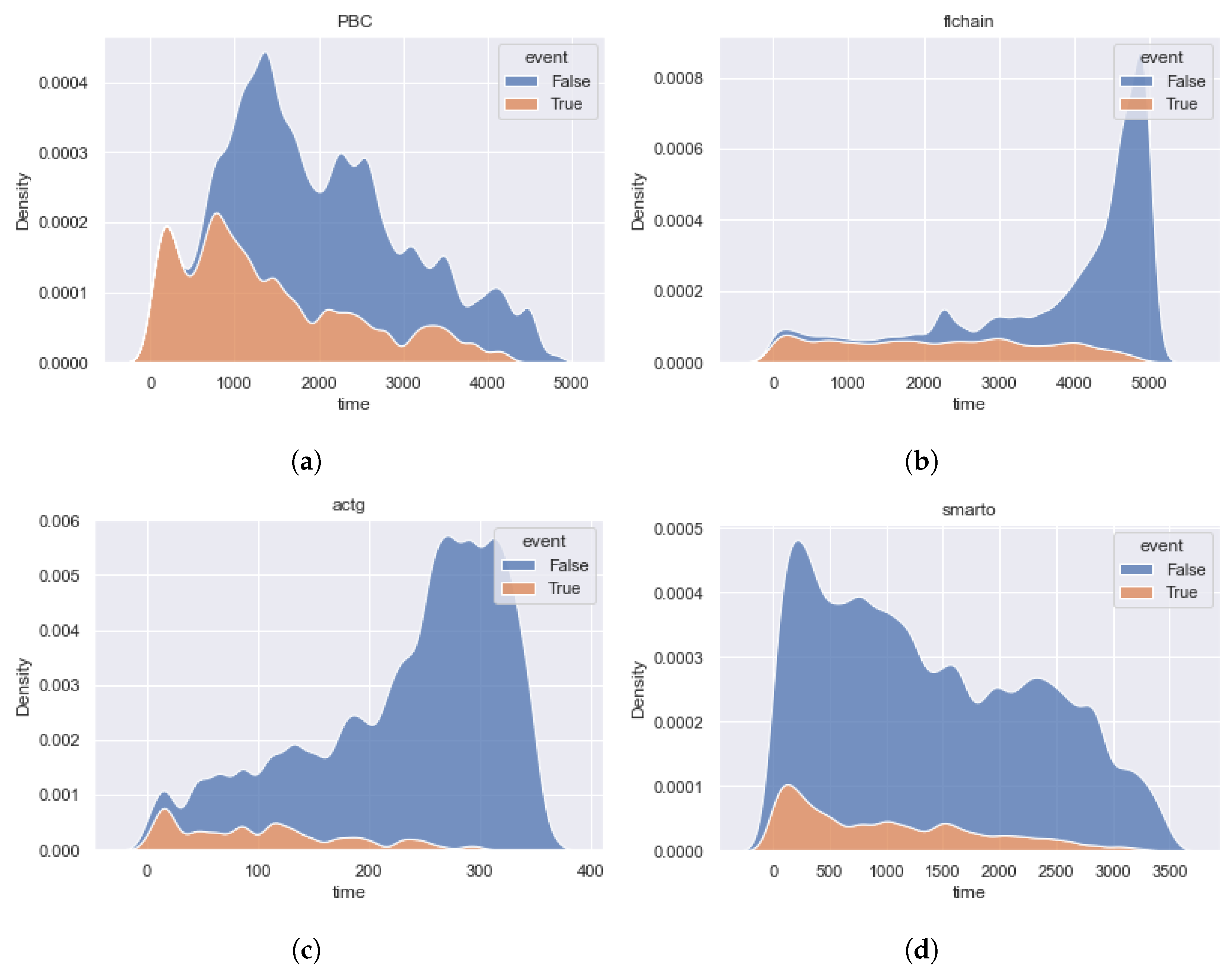
- The , , and datasets have a high imbalance of censored events and are uniform for the importance of event time contribution. It is important to note that for and datasets, the distribution of censoring time differs from the distribution of event time in the direction of increasing the importance of late events. The shapes of the dataset density functions are close.
5. Analysis of Biases in the Sensitivity of Metrics
- 1.
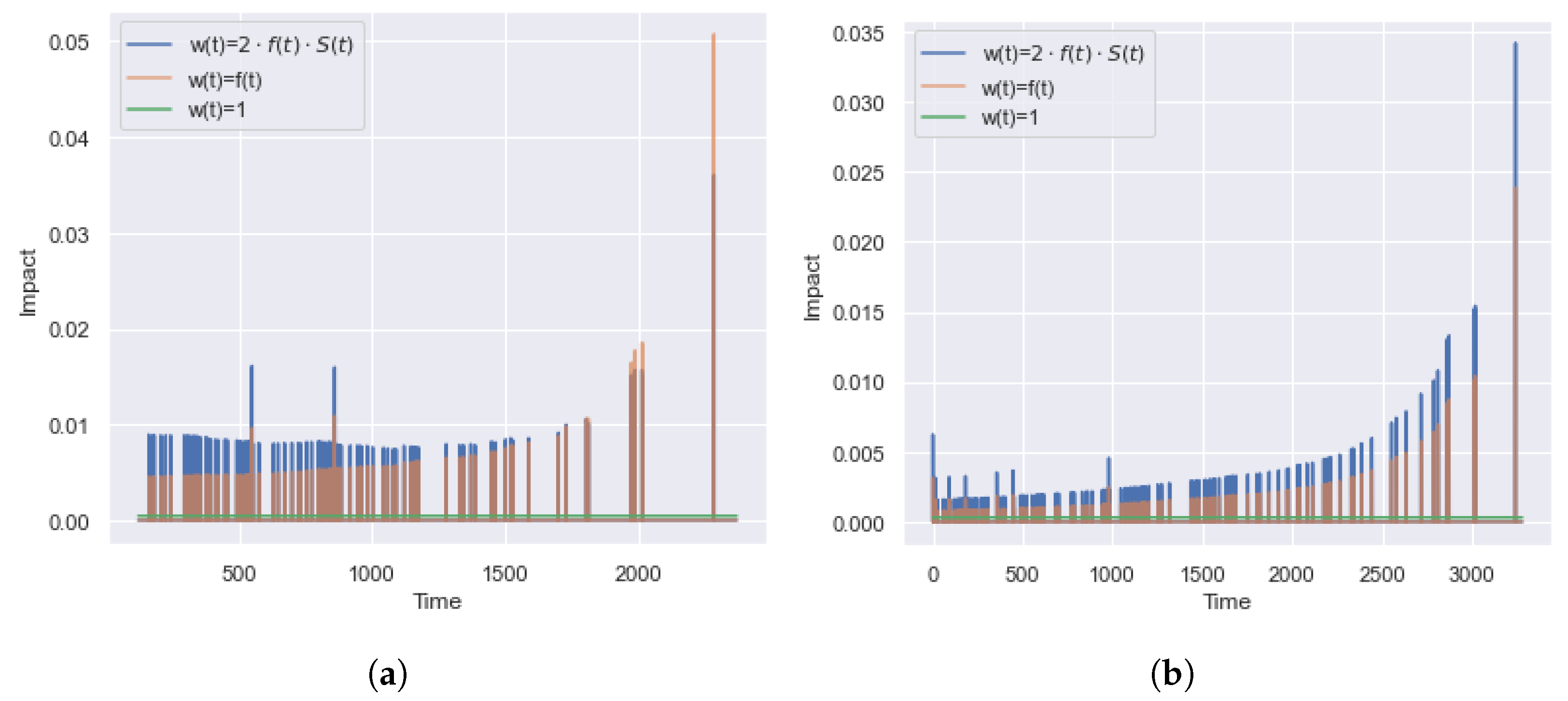
- The significance of the contribution of partial events (Section 5.1). The metric may have an implicit relationship between the contribution of events and its true time, which affects the reliability of the estimation. For example, the increased impact of late events is not suitable for data with dominant early events.
- 2.
- Dependence of integral metrics in time (Section 5.2). Integrated metric values may have a latent dependence on the timeline. In this case, the increased importance of a certain time period is not suitable for different data.
- 3.
- The influence of time variable in the integral metric (Section 5.3). The integrated variable directly affects aggregation over time and can lead to distortion of the significance of a certain period of time.
- 4.
- Resistance to the imbalance of censored observations (Section 5.4). The dominance of censoring can lead to false overstatement or understatement of the metric.
5.1. The Significance of the Contribution of Partial Events
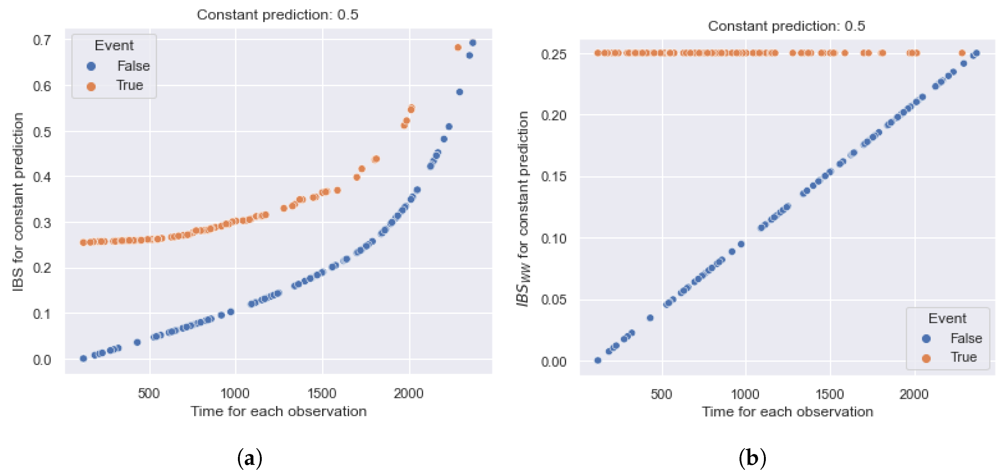
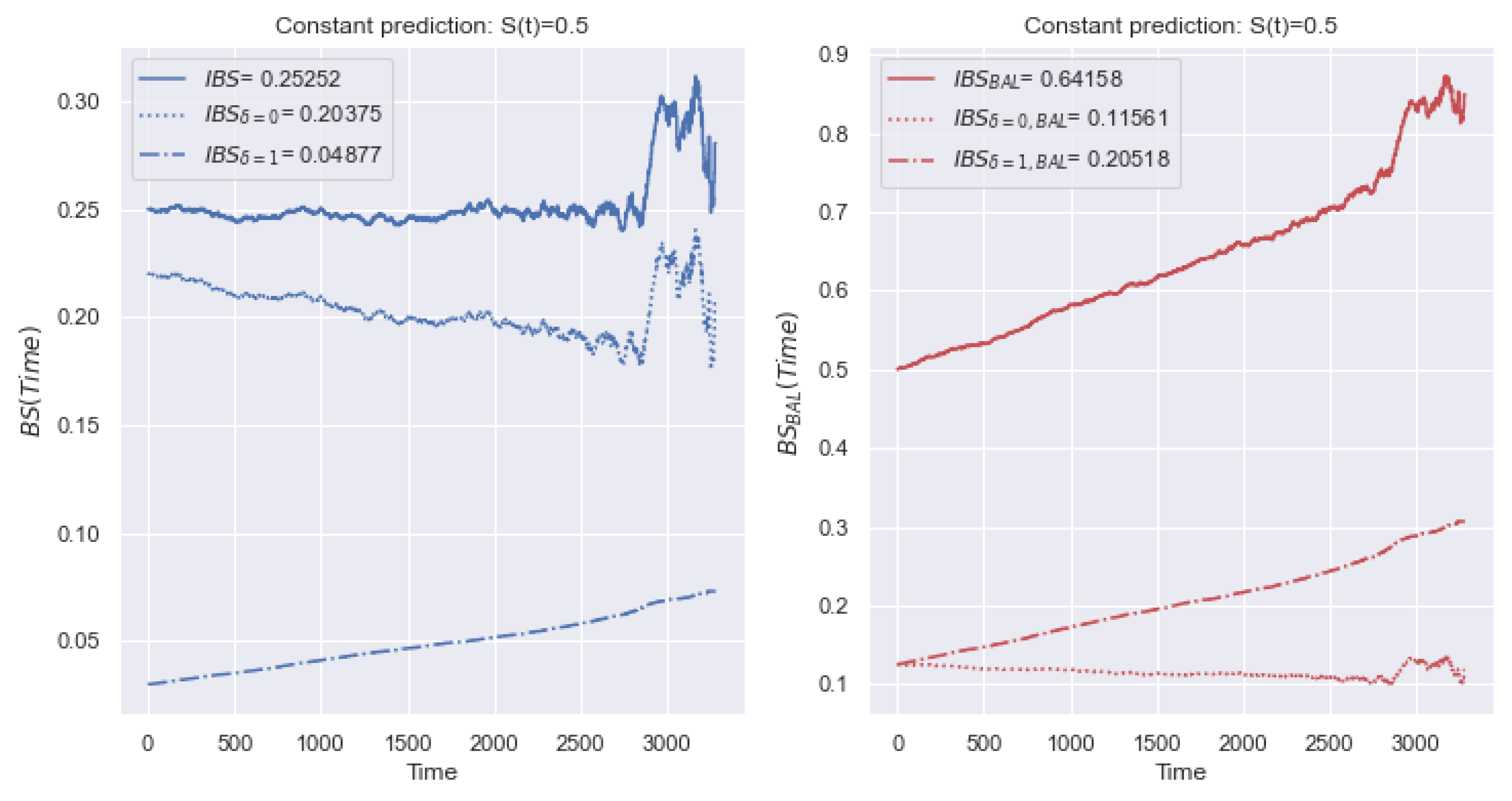
5.1.1. IBS
5.1.2. IAUC
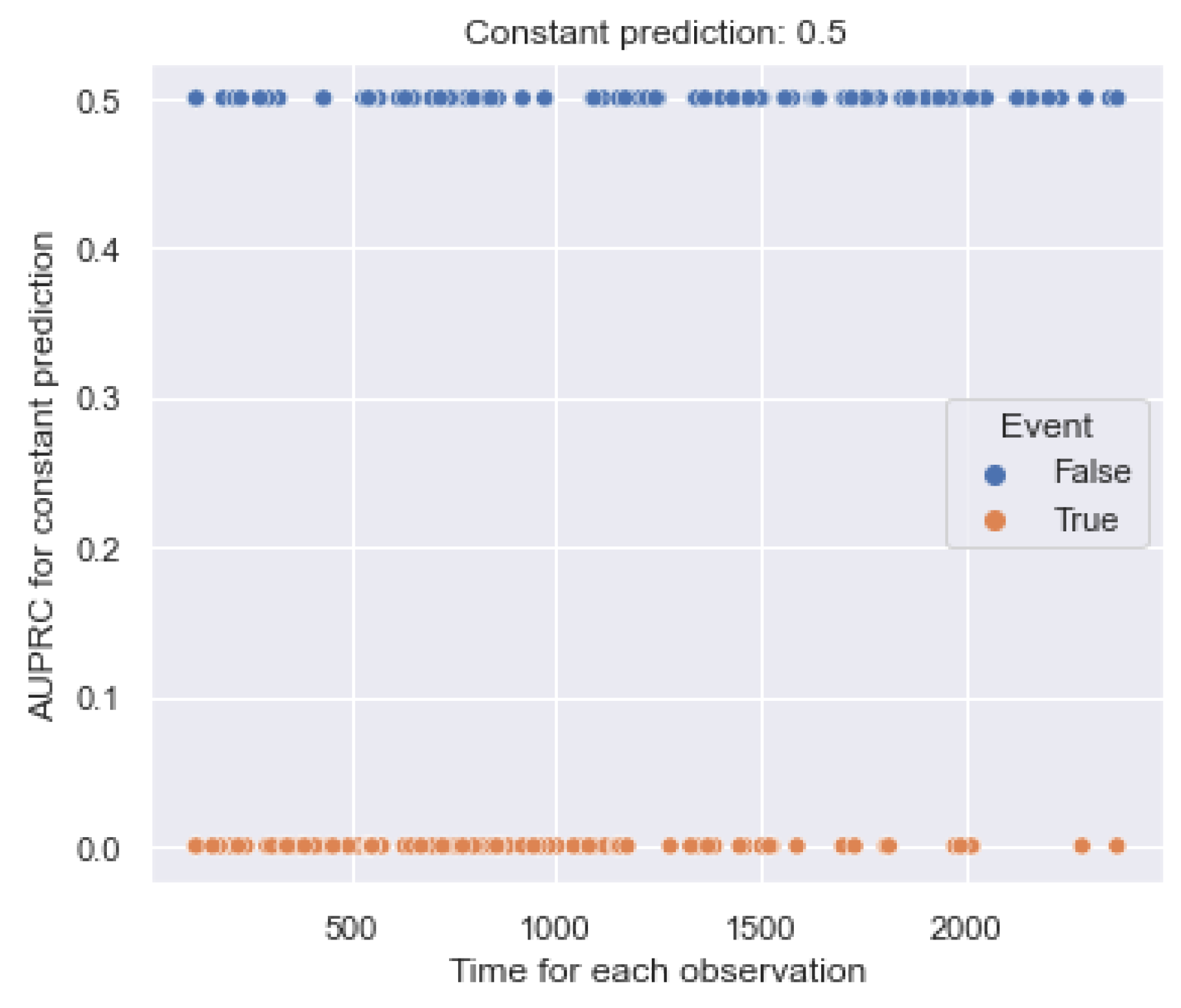
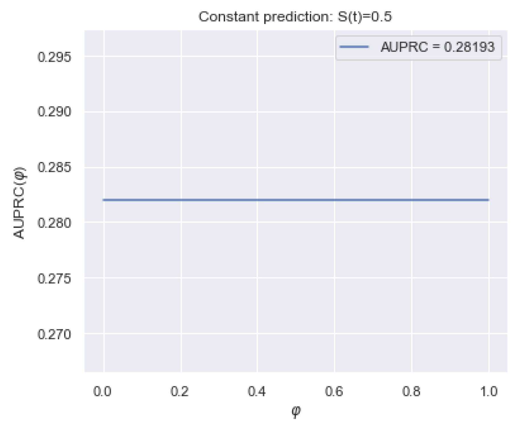
5.1.3. AUPRC
5.2. Dependence of Integral Metrics in Time
5.2.1. IBS
5.2.2. IAUC
5.2.3. AUPRC
5.3. The Influence of the Integration Variable
5.4. The Impact of the Imbalance
5.4.1. IBS
5.4.2. AUPRC
5.4.3. IAUC
5.5. Summary
6. Experiments
6.1. Experimental Setup
6.2. Results
6.3. Discussion of Hyperparameters
7. Conclusions
Author Contributions
Funding
Data Availability Statement
Conflicts of Interest
References
- Kleinbaum, D.; Klein, M. Survival Analysis: A Self-Learning Text, 3rd ed.; Statistics for Biology and Health; Springer: New York, NY, USA, 2016. [Google Scholar]
- Wang, P.; Li, Y.; Reddy, C.K. Machine learning for survival analysis: A survey. ACM Comput. Surv. (CSUR) 2019, 51, 1–36. [Google Scholar] [CrossRef]
- Lee, S.H. Weighted Log-Rank Statistics for Accelerated Failure Time Model. Stats 2021, 4, 348–358. [Google Scholar] [CrossRef]
- Karadeniz, P.G.; Ercan, I. Examining tests for comparing survival curves with right censored data. Stat Transit 2017, 18, 311–328. [Google Scholar]
- Lee, S.H. On the versatility of the combination of the weighted log-rank statistics. Comput. Stat. Data Anal. 2007, 51, 6557–6564. [Google Scholar] [CrossRef]
- Brendel, M.; Janssen, A.; Mayer, C.D.; Pauly, M. Weighted logrank permutation tests for randomly right censored life science data. Scand. J. Stat. 2014, 41, 742–761. [Google Scholar] [CrossRef]
- Hasegawa, T. Group sequential monitoring based on the weighted log-rank test statistic with the Fleming–Harrington class of weights in cancer vaccine studies. Pharm. Stat. 2016, 15, 412–419. [Google Scholar] [CrossRef]
- Kvamme, H.; Borgan, Ø. Continuous and discrete-time survival prediction with neural networks. Lifetime Data Anal. 2021, 27, 710–736. [Google Scholar] [CrossRef]
- Etikan, I.; Abubakar, S.; Alkassim, R. The Kaplan-Meier estimate in survival analysis. Biom. Biostat. Int. J. 2017, 5, 00128. [Google Scholar] [CrossRef]
- Andersen, P.K. Fifty years with the Cox proportional hazards regression model. J. Indian Inst. Sci. 2022, 102, 1135–1144. [Google Scholar] [CrossRef]
- Lin, D. On the Breslow estimator. Lifetime Data Anal. 2007, 13, 471–480. [Google Scholar] [CrossRef]
- Longato, E.; Vettoretti, M.; Di Camillo, B. A practical perspective on the concordance index for the evaluation and selection of prognostic time-to-event models. J. Biomed. Inform. 2020, 108, 103496. [Google Scholar] [CrossRef] [PubMed]
- Heagerty, P.J.; Zheng, Y. Survival model predictive accuracy and ROC curves. Biometrics 2005, 61, 92–105. [Google Scholar] [CrossRef] [PubMed]
- Lambert, J.; Chevret, S. Summary measure of discrimination in survival models based on cumulative/dynamic time-dependent ROC curves. Stat. Methods Med. Res. 2016, 25, 2088–2102. [Google Scholar] [CrossRef] [PubMed]
- Kvamme, H.; Borgan, Ø.; Scheel, I. Time-to-event prediction with neural networks and Cox regression. arXiv 2019, arXiv:1907.00825. [Google Scholar]
- Clim, A.; Zota, R.D.; TinicĂ, G. The Kullback-Leibler divergence used in machine learning algorithms for health care applications and hypertension prediction: A literature review. Procedia Comput. Sci. 2018, 141, 448–453. [Google Scholar] [CrossRef]
- Yari, G.; Mirhabibi, A.; Saghafi, A. Estimation of the Weibull parameters by Kullback-Leibler divergence of Survival functions. Appl. Math. Inf. Sci 2013, 7, 187–192. [Google Scholar] [CrossRef]
- Haider, H.; Hoehn, B.; Davis, S.; Greiner, R. Effective Ways to Build and Evaluate Individual Survival Distributions. J. Mach. Learn. Res. 2020, 21, 3289–3351. [Google Scholar]
- Avati, A.; Duan, T.; Zhou, S.; Jung, K.; Shah, N.H.; Ng, A.Y. Countdown regression: Sharp and calibrated survival predictions. In Proceedings of the Uncertainty in Artificial Intelligence, Virtual, 3–6 August 2020; pp. 145–155. [Google Scholar]
- Hastie, T.; Tibshirani, R.; Friedman, J.H.; Friedman, J.H. The Elements of Statistical Learning: Data Mining, Inference, and Prediction; Springer: Berlin/Heidelberg, Germany, 2009; Volume 2. [Google Scholar]
- Dormuth, I.; Liu, T.; Xu, J.; Yu, M.; Pauly, M.; Ditzhaus, M. Which test for crossing survival curves? A user’s guideline. BMC Med. Res. Methodol. 2022, 22, 34. [Google Scholar] [CrossRef]
- Bou-Hamad, I.; Larocque, D.; Ben-Ameur, H. A review of survival trees. Statist. Surv. 2011, 5, 44–71. [Google Scholar] [CrossRef]
- Ishwaran, H.; Kogalur, U.B.; Blackstone, E.H.; Lauer, M.S. Random survival forests. Ann. Appl. Stat. 2008, 2, 841–860. [Google Scholar] [CrossRef]
- Vasilev, I.; Petrovskiy, M.; Mashechkin, I.V. Survival Analysis Algorithms based on Decision Trees with Weighted Log-rank Criteria. In Proceedings of the 11th International Conference on Pattern Recognition Applications and Methods, Virtual, 3–5 February 2022; pp. 132–140. [Google Scholar]
- Pölsterl, S. scikit-survival: A Library for Time-to-Event Analysis Built on Top of scikit-learn. J. Mach. Learn. Res. 2020, 21, 1–6. [Google Scholar]
- Nguyen, N.P. Gradient Boosting for Survival Analysis with Applications in Oncology; University of South Florida: Tampa, FL, USA, 2019. [Google Scholar]
- Drysdale, E. SurvSet: An open-source time-to-event dataset repository. arXiv 2022, arXiv:2203.03094. [Google Scholar]
- Schumacher, M. Rauschecker for the german breast cancer study group, randomized 2× 2 trial evaluating hormonal treatment and the duration of chemotherapy in node-positive lbreast cancer patients. J. Clin. Oncol. 1994, 12, 2086–2093. [Google Scholar] [CrossRef]
- Royston, P.; Lambert, P.C. Flexible Parametric Survival Analysis Using Stata: Beyond the Cox Model; Stata Press: College Station, TX, USA, 2011; Volume 347. [Google Scholar]
- Knaus, W.A.; Harrell, F.E.; Lynn, J.; Goldman, L.; Phillips, R.S.; Connors, A.F.; Dawson, N.V.; Fulkerson, W.J.; Califf, R.M.; Desbiens, N.; et al. The SUPPORT prognostic model: Objective estimates of survival for seriously ill hospitalized adults. Ann. Intern. Med. 1995, 122, 191–203. [Google Scholar] [CrossRef] [PubMed]
- Yan, L.; Zhang, H.T.; Goncalves, J.; Xiao, Y.; Wang, M.; Guo, Y.; Sun, C.; Tang, X.; Jing, L.; Zhang, M.; et al. An interpretable mortality prediction model for COVID-19 patients. Nat. Mach. Intell. 2020, 2, 283–288. [Google Scholar] [CrossRef]
- Kaplan, M.M. Primary biliary cirrhosis. N. Engl. J. Med. 1996, 335, 1570–1580. [Google Scholar] [CrossRef] [PubMed]
- Simons, P.C.G.; Algra, A.; Van De Laak, M.; Grobbee, D.; Van Der Graaf, Y. Second manifestations of ARTerial disease (SMART) study: Rationale and design. Eur. J. Epidemiol. 1999, 15, 773–781. [Google Scholar] [CrossRef]
- Hammer, S.M.; Squires, K.E.; Hughes, M.D.; Grimes, J.M.; Demeter, L.M.; Currier, J.S.; Eron, J.J., Jr.; Feinberg, J.E.; Balfour, H.H., Jr.; Deyton, L.R.; et al. A controlled trial of two nucleoside analogues plus indinavir in persons with human immunodeficiency virus infection and CD4 cell counts of 200 per cubic millimeter or less. N. Engl. J. Med. 1997, 337, 725–733. [Google Scholar] [CrossRef]
- Kyle, R.A.; Therneau, T.M.; Rajkumar, S.V.; Larson, D.R.; Plevak, M.F.; Offord, J.R.; Dispenzieri, A.; Katzmann, J.A.; Melton, L.J., III. Prevalence of monoclonal gammopathy of undetermined significance. N. Engl. J. Med. 2006, 354, 1362–1369. [Google Scholar] [CrossRef]
- Hung, H.; Chiang, C.T. Estimation methods for time-dependent AUC models with survival data. Can. J. Stat. 2010, 38, 8–26. [Google Scholar] [CrossRef]
- Uno, H.; Cai, T.; Tian, L.; Wei, L.J. Evaluating prediction rules for t-year survivors with censored regression models. J. Am. Stat. Assoc. 2007, 102, 527–537. [Google Scholar] [CrossRef]
- Chawla, N.V. Data mining for imbalanced datasets: An overview. In Data Mining and Knowledge Discovery Handbook; Springer: New York, NY, USA, 2010; pp. 875–886. [Google Scholar]
- He, H.; Ma, Y. Imbalanced Learning: Foundations, Algorithms, and Applications; Wiley-IEEE Press: Hoboken, NJ, USA, 2013. [Google Scholar]
- Fawcett, T. An introduction to ROC analysis. Pattern Recognit. Lett. 2006, 27, 861–874. [Google Scholar] [CrossRef]
- Tong, L.I.; Chang, Y.C.; Lin, S.H. Determining the optimal re-sampling strategy for a classification model with imbalanced data using design of experiments and response surface methodologies. Expert Syst. Appl. 2011, 38, 4222–4227. [Google Scholar] [CrossRef]
- Chen, Y.; Jia, Z.; Mercola, D.; Xie, X. A gradient boosting algorithm for survival analysis via direct optimization of concordance index. Comput. Math. Methods Med. 2013, 2013, 873595. [Google Scholar] [CrossRef] [PubMed]
- Binder, H.; Binder, M.H. Package ‘CoxBoost’. 2015. Available online: https://cran.r-hub.io/web/packages/CoxBoost/CoxBoost.pdf (accessed on 20 August 2023).
- Bai, M.; Zheng, Y.; Shen, Y. Gradient boosting survival tree with applications in credit scoring. J. Oper. Res. Soc. 2022, 73, 39–55. [Google Scholar] [CrossRef]
- Refaeilzadeh, P.; Tang, L.; Liu, H. Cross-validation. Encycl. Database Syst. 2009, 5, 532–538. [Google Scholar]


| Name | N | Feat | Cens, Event | Event (%) | NaN (Feat) |
|---|---|---|---|---|---|
| [30] | 9105 | 35 | (2904, 6201) | 0.681 | 21 |
| [31] | 375 | 224 | (201, 174) | 0.464 | 222 |
| [28] | 686 | 8 | (387, 299) | 0.436 | 0 |
| [29] | 2982 | 11 | (1710, 1272) | 0.427 | 0 |
| [32] | 418 | 17 | (257, 161) | 0.385 | 12 |
| [35] | 7874 | 10 | (5705, 2169) | 0.275 | 1 |
| [33] | 3873 | 26 | (3413, 460) | 0.119 | 16 |
| [34] | 1151 | 11 | (1055, 96) | 0.083 | 0 |
| Metric Name | Section 5.1 | Section 5.2 | Section 5.3 | Section 5.4 | G(T) |
|---|---|---|---|---|---|
| + | + | - | + | + | |
| - | + | - | + | - | |
| - | - | - | + | - | |
| + | + | - | - | + | |
| - | + | - | - | - | |
| - | - | - | - | - | |
| ? | - | + | - ? | + | |
| ? | - | + | - ? | + | |
| ? | - | - | - ? | + | |
| - | - | - | + | - | |
| - | - | - | - | - |
| Model Name | Hyperparameter | Grid |
|---|---|---|
| CoxPH Survival Analysis | regularization penalty | 0.1, 0.01, 0.001 |
| ties | breslow, efron | |
| Survival Tree | split strategy | best, random |
| max depth | from 10 to 30 step 5 | |
| min sample leaf | from 1 to 20 step 1 | |
| max features | sqrt, log2, none | |
| Random Survival Forest | num estimators | from 10 to 100 step 10 |
| max depth | from 10 to 30 step 5 | |
| min sample leaf | from 1 to 20 step 1 | |
| max features | sqrt, log2, none | |
| Component-wise Gradient Boosting | num estimators | from 10 to 100 step 10 |
| learning rate | from 0.01 to 0.5 step 0.01 | |
| subsample | from 0.5 to 1.0 step 0.1 | |
| dropout rate | from 0.0 to 0.5 step 0.1 | |
| Gradient Boosting SA | num estimators | from 10 to 100 step 10 |
| max depth | from 10 to 30 step 5 | |
| min sample leaf | from 1 to 20 step 1 | |
| max features | sqrt, log2, none | |
| learning rate | from 0.01 to 0.5 step 0.01 | |
| Bagging | bootstrap sample size | from 0.5 to 1.0 step 0.1 |
| num estimators | from 10 to 50 step 10 | |
| max depth | from 10 to 30 step 5 | |
| min sample leaf | 0.05, 0.001 | |
| max features | 0.3, sqrt | |
| leaf model | KM, KM10 (Section 2.2.1) | |
| criterion | maxcombo, peto, tarone-ware, wilcoxon, logrank |
| DATASET | |||
|---|---|---|---|
| , | , | , | |
| , | , | , | |
| , | , | ||
| , | , | , | |
| , | , | ||
| no winner | no winner | no winner | |
| , | , | , | |
| , | , | , | |
| Total |
Disclaimer/Publisher’s Note: The statements, opinions and data contained in all publications are solely those of the individual author(s) and contributor(s) and not of MDPI and/or the editor(s). MDPI and/or the editor(s) disclaim responsibility for any injury to people or property resulting from any ideas, methods, instructions or products referred to in the content. |
© 2023 by the authors. Licensee MDPI, Basel, Switzerland. This article is an open access article distributed under the terms and conditions of the Creative Commons Attribution (CC BY) license (https://creativecommons.org/licenses/by/4.0/).
Share and Cite
Vasilev, I.; Petrovskiy, M.; Mashechkin, I. Sensitivity of Survival Analysis Metrics. Mathematics 2023, 11, 4246. https://doi.org/10.3390/math11204246
Vasilev I, Petrovskiy M, Mashechkin I. Sensitivity of Survival Analysis Metrics. Mathematics. 2023; 11(20):4246. https://doi.org/10.3390/math11204246
Chicago/Turabian StyleVasilev, Iulii, Mikhail Petrovskiy, and Igor Mashechkin. 2023. "Sensitivity of Survival Analysis Metrics" Mathematics 11, no. 20: 4246. https://doi.org/10.3390/math11204246
APA StyleVasilev, I., Petrovskiy, M., & Mashechkin, I. (2023). Sensitivity of Survival Analysis Metrics. Mathematics, 11(20), 4246. https://doi.org/10.3390/math11204246