Abstract
Many-objective optimization is a critical research topic in the evolutionary computing community. Many algorithms have been proposed to tackle this problem, with evolutionary algorithms based on the hypervolume being among the most effective ones. However, calculating the hypervolume indicator in high-dimensional objective spaces remains time-consuming. To address this issue, we propose a two-stage hypervolume-based evolutionary algorithm (ToSHV) that separates global search and local search to ensure both convergence and diversity. ToSHV performs a global search in the first stage by generating multiple offspring per generation. We modified the R2HCA method to estimate the overall hypervolume contribution, avoiding the time-consuming nature of updating the hypervolume contribution with the greedy method. In the second stage, only one offspring is produced per generation to emphasize local exploration and enhance population diversity. Furthermore, a stage-switching mechanism is designed to dynamically select the appropriate search mode based on the prevailing population distribution. We evaluate our algorithm on WFG and DTLZ test suites, comparing it with three hypervolume-based algorithms and four state-of-the-art algorithms. Experimental results show that our approach is competitive in most cases.
Keywords:
many-objective optimization; evolutionary algorithm; hypervolume contribution approximation MSC:
68W50; 90C29
1. Introduction
A multi-objective optimization problem (MOP) involves simultaneously optimizing multiple objectives that are typically mutually exclusive; improving one objective often leads to the deterioration of another. Unlike single-objective optimization problems, the optimal solution to an MOP is a set known as the Pareto set. In recent years, many evolutionary multi-objective algorithms (EMOAs) have been developed to solve MOPs, yielding satisfactory results. However, many real-world problems, which are known as many-objective optimization problems (MaOPs), have more than three optimization objectives [1]. The emergence of MaOPs poses a challenge for existing evolutionary algorithms. Based on their mechanisms, EMOAs can be categorized into three groups: Pareto-based, decomposition-based, and indicator-based approaches.
Pareto-based EMOAs employ Pareto dominance as the screening criterion for environmental selection [2,3,4]. These algorithms have simple rules, run quickly, and perform well when dealing with MOPs with two or three objectives. However, in MaOPs, the proportion of non-dominated solutions in the offspring increases as the dimension of the objective space grows. When the solution space has more than 10 dimensions, all offspring generated are non-dominated solutions, rendering the Pareto dominance relationship ineffective and weakening the environmental selection pressure. To address this issue, researchers have proposed new dominance relationships, such as -dominance [5], r-dominance [6], and -dominance [7]. These new relationships improve the ability of Pareto-based EMOAs to handle MaOPs.
Decomposition-based EMOAs transform an MOP into multiple single-objective problems (SOPs) and optimize them simultaneously [8,9,10,11,12]. In solving MOPs, two important solution set characteristics must be considered: convergence and diversity. Decomposition-based EMOAs achieve diversity by evenly dividing the objective space into multiple subspaces, so that only the convergence of each subspace needs to be considered during optimization. However, the Pareto front (PF) of real-world problems may be irregular [13], with features such as disconnection, degradation, or weak Pareto. An evenly distributed weight vector can result in an uneven distribution of the solution set over the PF. For MaOPs, where the objective space is high-dimensional, the PF may be a combination of the aforementioned features. To address these issues, researchers have designed weight vector adaptive strategies that adjust the weight vector according to the distribution of solutions in the running process of the algorithm [14,15,16].
Indicator-based EMOAs transform MOPs into SOPs by introducing population evaluation indicators [17,18,19]. Evaluation indicators, such as hypervolume [20], inverted generational distance (IGD) [21], R2 [22], etc., take into account both the convergence and diversity of the population and return a real number representing the quality of the solution set. Unlike the other two types of EMOAs, indicator-based EMOAs are not affected by the shape of the PF and the dimension of the problem, which allows them to obtain a more evenly distributed solution set. However, most known indicators require setting parameters, and the appropriate parameter settings directly affect the distribution of the solution sets. For instance, if the reference point of hypervolume is set too close to the PF, the solutions are concentrated in the central region of the PF; conversely, if the reference point is set too far away from the PF, the solutions are concentrated at the edge of the PF [23]. Parameter adaptation of indicators is a hot topic in the evolutionary computing community.
Among various performance indicators, hypervolume is a popular choice for EMOAs due to its strict adherence to the Pareto dominance relation and its independence from prior problem knowledge. Many hypervolume-based EMOAs have been proposed and have shown satisfactory performance on both MOPs and MaOPs. For MOPs, hypervolume accuracy is crucial, and algorithms like SMS-EMOA [24] and FV-MOEA [25] that achieve accurate hypervolume solutions are often used. For MaOPs, where accurate hypervolume solutions are time-consuming to compute, approximation algorithms like HypE [26] and R2HCA-MOEA [27] are typically employed. EMOAs can also be categorized based on their evolution strategy as () or () approaches, each with their own unique characteristics:
- The () evolutionary strategy produces a single offspring in each iteration, leading to a gradual improvement in the quality of the solution set. However, this strategy has two drawbacks. Firstly, producing only one offspring at a time increases the risk of getting trapped in local optima. Secondly, when generating the same number of offspring, the () strategy takes longer to compute than the () evolutionary strategy;
- The () evolutionary strategy generates multiple offspring each time, which improves its global search ability. However, this introduces a new problem called the hypervolume subset selection problem (HSSP). To address this problem, a greedy algorithm is typically used, which requires recalculating the hypervolume contribution of each solution in the solution set every time a descendant is eliminated. This increases the running time of the algorithm.
Given the challenges posed by the two aforementioned evolutionary strategies, a logical approach would be to amalgamate them, thereby harnessing the benefits of each. In this article, we propose a two-stage EMOA based on the hypervolume. In the first stage, the algorithm employs the () evolutionary strategy to emphasize global search. In the second stage, the () evolutionary strategy is used to prioritize local search. It is important to note that the two stages are not rigidly defined and switch dynamically based on the state of the solution set during the algorithm’s operation. The main contributions of this paper are listed as follows:
- A two-stage hypervolume-based EMOA framework that combines the advantages of () and () evolutionary strategies for MaOPs is proposed. Additionally, we designed a stage-switching mechanism to dynamically adapt the evolutionary strategies based on the current state of the population;
- To reduce the time consumed by the greedy algorithm in the () evolutionary strategy, we introduce an environmental selection strategy based on the overall hypervolume contribution. By calculating the overall hypervolume contribution of each solution, we can quickly achieve a coarse-grained screening of the population;
- The effectiveness of the proposed algorithm is evaluated by comparing it with three hypervolume-based EMOAs and four advanced EMOAs using the WFG and DTLZ test sets with 5, 10, and 15 dimensions. Experimental results demonstrate that the proposed algorithm is competitive.
2. Preliminaries
2.1. Hypervolume
Hypervolume is a popular performance indicator in MOPs that measures the quality of a set of solutions. It is based on the volume of the portion of the objective space that is dominated by the solutions. In other words, it measures the amount of objective space that is covered by the solutions and not dominated by any other solutions. The hypervolume is computed by integrating the objective space volume that is dominated by a given set of candidate solutions with respect to a reference point. Mathematically, the hypervolume of a set of candidate solutions S with respect to a reference point can be represented as
where m is the number of objectives, is the i-th component of the reference point, is an indicator function that equals 1 if is dominated by a solution in S and 0 otherwise. The higher the hypervolume value, the better the solution set is considered to be. Hypervolume has been widely used as a performance indicator for evaluating and comparing multi-objective optimization algorithms.
2.2. Hypervolume Contribution
Hypervolume contribution is a measure of how much a single solution contributes to the hypervolume indicator value of a set of solutions. It represents the portion of the hypervolume indicator that is covered by a single solution. Solutions with higher hypervolume contributions are considered more important in terms of improving the overall quality of the solution set. Mathematically, the hypervolume contribution of a solution a in S with respect to a reference point can be represented as
2.3. Overall Hypervolume Contribution
The last concept is the overall hypervolume contribution. Because the general hypervolume contribution only considers the measure of the area dominated by the current solution alone but ignores the area dominated by other solutions, the overall hypervolume contribution considers this impact and is expressed as follows:
where represents the worst value in each dimension in the objective point set. For example, a minimization problem represents the maximum objective value in each dimension, while a maximization problem does the opposite. A solution’s total hypervolume contribution comprises the area it independently dominates, along with an equitable share of the region it jointly dominates with other solutions. This observation led to the idea of considering the expected loss in hypervolume that can be attributed to a particular solution when exactly multiple solutions are removed. Figure 1 shows the geometric interpretation of each of the three concepts.

Figure 1.
Geometric illustration of basic concepts. (a) The hypervolume of set . (b) The hypervolume contribution of solution in set S. (c) The overall hypervolume contribution of solution in set S.
3. Proposed Algorithm
3.1. Framework
The pseudocode of the ToSHV algorithm framework is shown in Algorithm 1. The algorithm starts with an initialization operation (lines 1–3), where the population and direction vectors are randomly generated. The variable “Stage” determines the current operation process of the algorithm cycle. By default, “Stage” is set to 1, which means that the algorithm first executes the operations of Stage-I. In each iteration of the main loop, only one stage of operations is executed. Stage-I mainly performs coarse-grained global search, which rapidly improves the convergence of the solution set. When the solution set remains non-dominated for multiple consecutive generations, it indicates that the algorithm is approaching the PF or a local PF. In this case, the algorithm switches to Stage-II for fine-grained local search, which aims to increase the diversity of the population. If a dominant solution is found during this stage, it indicates that the current population can escape from the local optima. At this point, the algorithm switches back to Stage-I to continue the global search. To provide a more intuitive representation of the algorithm process, we include a flowchart of the algorithm, depicted in Figure 2.
| Algorithm 1 The framework of ToSHV |
| Require: Population Size, N; Direction Vector Number, ; Maximum Function Evaluations Number, FEs; Ensure: Final Population, P;
|

Figure 2.
Flowchart of ToSHV framework.
3.2. Stage-I: Global Search with ( + ) Evolutionary Strategy
Algorithm 2 shows the pseudocode of the search process in Stage-I. Firstly, N offspring are generated using a binary tournament selection method (line 1). It is worth noting that the fitness of an individual in the tournament is defined as its rank level after non-dominated sorting. Next, the children are merged with the parents to form a combined set, which is then sorted using non-domination (lines 2–3). Starting from the first rank, solutions are successively added to the new-generation population until the total size exceeds N. Finally, the overall hypervolume contribution of each solution in the last rank is computed, and the smallest solutions are removed until the population size is reduced to N (lines 4–5). This process is designed to handle scenarios with multiple ranks after non-dominated sorting, which are typically encountered during the early stages of the search process. By using the () evolutionary strategy, the algorithm can efficiently improve convergence and maintain diversity, thereby avoiding getting stuck in local optima.
| Algorithm 2 Stage-1 process |
| Require: Population, P; Direction Vector Number, ; Ensure: Selected Population, P;
|
Due to the time-consuming nature of precisely calculating the overall hypervolume contribution of the MaOP, an approximate estimation method is employed instead. Further details on this method will be discussed in Section 3.4. It is worth noting that the overall hypervolume contribution used in Stage-I for one-off offspring selection does not guarantee an optimal HSSP. The reason for adopting this mechanism is that the solutions in the first few ranks, which are most valuable for improving convergence, have already been included in the new-generation population after non-dominated sorting. Therefore, it is only necessary to ensure the diversity of the last rank, and approximate calculations are sufficient.
3.3. Stage-II: Local Search with ( + 1) Evolutionary Strategy
When non-dominated solutions are obtained for an extended period in the first stage, it indicates that the algorithm has converged to the PF or local PF. In this case, it is necessary to proceed to the second stage for local search to enhance the diversity of the population. In Stage-II, the ( + 1) evolutionary strategy is employed to steadily improve the quality of the solution set. The pseudocode for Stage-II is presented in Algorithm 3. Firstly, similar to Stage-I, two parents are selected using binary tournament, and an offspring is generated using binary crossover and polynomial mutation (line 1). It should be noted that the fitness of an individual in this stage adopts the hypervolume contribution of each solution. This implies that solutions with higher hypervolume contributions are assigned more computational resources and are locally searched in their decision space. This is intuitive because a solution with a large hypervolume contribution means that it is far from other solutions and a local search at its location has a higher chance of obtaining a solution that enhances the population’s diversity. Secondly, consistent with the general ( + 1) EMOA, N + 1 solutions are computed for each solution’s hypervolume contribution, and the smallest one is discarded (lines 2–4). The R2HCA method, introduced in [28], is used for calculating the hypervolume contribution of each solution. The detailed steps of this method will be explained in Section 3.4.
| Algorithm 3 Stage-2 process |
| Require: Population, P; Direction Vector Number, ; Ensure: Selected Population, P;
|
3.4. Hypervolume Contribution Approximation
In this subsection, we will provide a detailed introduction to the hypervolume approximation methods used in the two stages mentioned above. Firstly, we briefly introduce the R2HCA algorithm proposed in [28], which is mainly utilized to approximate the hypervolume contribution of each solution in the solution set. Then, we explain how R2HCA can be slightly modified to approximate the overall hypervolume contribution of each solution in the population, as introduced in our previous work [29].
R2HCA is a line-based method for approximating hypervolume contribution. Unlike the Monterallo method, this approach approximates a solution’s hypervolume contribution by measuring its distance to the hypervolume plane in various directions, as shown in Figure 3a. The method involves generating uniformly distributed direction vectors in the first quadrant and then computing the approximate hypervolume contribution of each solution using the following formula:

Figure 3.
Illustration of R2HCA principle. (a) The basic idea of R2HCA. (b) The geometric meaning of the variables in the calculation process.
In this method, is the set of direction vectors, and a is the solution whose hypervolume contribution needs to be approximated from solution set S. The quantity is the Euclidean distance from a to the hypervolume plane along direction vector , while represents the distance from a to the area enclosed by reference point r along direction vector . Figure 3b illustrates the geometric interpretation of and in the target space. For minimization problems, the two quantities are computed as follows:
R2HCA is primarily used to approximate the hypervolume contribution in Stage-II, and we modify it in order to make it approximate the overall hypervolume contribution required in Stage-I. The overall process can be divided into four steps:
- First, when solving for , all values of , are kept, not just the minimum as in R2HCA.
- Next, the value of is calculated; values that are greater than are excluded; and the remaining values are arranged in ascending order, with being the last value on the list. The specific steps are illustrated in Figure 4a.
 Figure 4. Illustration of the modification of R2HCA. (a) Exclude operation of R2 data array. (b) Adjusted R2 data array format.
 - Then, based on the first two steps, data for all direction vectors are obtained and arranged into an irregular data matrix, as shown in Figure 4b.
- Finally, each column of data is summed in turn, and the mean value is taken, with the obtained mean values then being summed.
The modification of R2HCA aims to approximate the overall hypervolume contribution by utilizing the intersection information of direction vectors with different regions of the hypervolume. In the second step, we remove some intersection points that fall outside the hypervolume region, such as in Figure 3b. By obtaining and arranging all intersection information in ascending order, we can use these data to estimate the overall hypervolume contribution. Passing through each intersection point means that the direction vector enters a new hypervolume area and increases the number of common dominant solutions in that area by one. Additionally, it should be noted that we have adopted the Tensor and its update mechanism used in [27] to simplify the calculation and achieve faster running speed for our algorithm.
3.5. Computational Complexity
The running time of ToSHV is mainly attributed to the two stages it involves. As the evolutionary strategies of these stages are different, we aim to provide a unified analysis of the time complexity required to generate N offspring. For Stage-I, only one generation is needed to produce N offspring. Specifically, the computational complexity of generating offspring is , while the computation complexity of non-dominated sorting is . The complexity of computing hypervolume contribution is , and the environmental selection complexity is . Taken together, the computational complexity of the Stage-I operation is . For Stage-II, generating N descendants requires N generations. The generation complexity of the offspring is , and the computational complexity of non-dominated sorting is . The complexity of calculating the hypervolume contribution is , and the environmental selection complexity is . Therefore, the computational complexity of the Stage-II operation is . In summary, the computational complexity of the entire ToSHV algorithm is .
4. Experimental Design and Analysis
4.1. Experiment Settings
4.1.1. Test Problems
To comprehensively evaluate the proposed method, we conducted experiments using the WFG [30] and DTLZ [21] test sets. The WFG test set comprises WFG 1–9 with objective dimensions of 5, 10, and 15. The number of decision variables was set to 18 + 2 × m, and the maximum function evaluations number, FEmax, was set to 100,000. Similarly, for the DTLZ test set, we included DTLZ 1–7, along with IDTLZ1 and IDTLZ2 [13]. The number of decision variables for DTLZ1 and IDTLZ1 was set to 4+m, while for others, it was set to 9+m, with FEmax set to 30,000. The remaining settings were similar to the WFG test set.
4.1.2. Platforms
The experimental part of this paper was implemented on the PlatEMO platform [31], an open-source project based on Matlab. The comparative algorithms introduced later are also included in the algorithm source code provided by PlatEMO. In addition, the calculation of indicators and parameter settings were also based on the settings in the PlatEMO platform. The computer used for conducting the simulation experiments had the following specifications: CPU: Intel Core i5 8500; RAM: 16 GB.
4.1.3. Parameter Settings
The population size (N) was set to 100 for all test problems. The maximum number of function evaluations, FEmax, was used as the termination condition of the algorithm, and the specific settings are introduced in the previous subsection. We used SBX and polynomial mutation with a distribution index of 20 for both operators. The crossover rate is set to 1.0 and the mutation rate was set to 1/n, where n is the number of decision variables. Each algorithm was evaluated on each test problem 30 times with independent runs.
4.1.4. Performance Metrics
We employed two evaluation metrics, hypervolume and inverse generational distance (IGD). The calculation formula for hypervolume is given in Equation (1), and we set its reference point to . It should be noted that due to the complexity of hypervolume calculation, we used the Montelaro method to compute the hypervolume for the 5-, 10-, and 15-dimensional objective spaces with 10,000 sampling points.
IGD [21] provides combined information about convergence and diversity. The difference from HV is that a lower IGD value means a better solution quality. It is calculated as
The reference point for IGD was set to the default value provided by the PlatEMO platform. Furthermore, we performed a Wilcoxon rank-sum test. The Wilcoxon rank-sum test was conducted with a significance level of 5% on the experimental results to determine whether the proposed algorithm differs significantly from the other comparative algorithms. The symbols “+”, “−”, and “≈” represent that the compared EMOA is “significantly better than”, “significantly worse than”, and “statistically similar to” ToSHV, respectively.
4.1.5. Compared Algorithms
We selected two sets of comparative algorithms to comprehensively test the performance of ToSHV. For the first group of comparison algorithms, we chose three hypervolume-based EMOAs, since ToSHV is also a hypervolume-based algorithm. In the second group, we set four advanced EMOAs based on other mechanisms to test the comprehensive performance of ToSHV. The following is a brief introduction to them:
- HypE [26] is a hypervolume-based algorithm that aims to maximize the hypervolume of the Pareto set. It uses the Monte Carlo method to estimate the hypervolume contribution of each individual in the population and selects parents for the next generation based on their hypervolume contributions. It also employs a niching mechanism to maintain diversity among the population.
- SMS-EMOA [24] is an EMOA based on S-metric environmental selection and () evolution strategy. In each generation, the algorithm generates only one offspring to ensure the quality and steady growth of the population.
- R2HCA-EMOA [27] is similar to SMS-EMOA in that it uses the () evolutionary strategy and hypervolume contribution as the environmental selection criterion. However, it differs in that it approximates the hypervolume of each solution using the R2HCA algorithm. Additionally, it introduces a special data structure and update mechanism to simplify computational complexity.
- NSGA-III [9] is a decomposition-based EMOA. It uses a modified non-dominated sorting approach to deal with many objectives, where the population is divided into multiple layers based on their non-domination levels. The algorithm uses a reference point approach to encourage diversity and to avoid crowding in the decision space. The reference points are updated dynamically during the evolutionary process to provide a balanced distribution of solutions along the Pareto front.
- MOEA/DD [10] combines dominance- and decomposition-based approaches, for many-objective optimization. It is to exploit the merits of both dominance- and decomposition-based approaches to balance the convergence and diversity of the evolutionary process.
- DGEA [32] is an adaptive offspring generation method for large-scale multi-objective optimization. It adaptively employs two sets of direction vectors to generate descendant solutions. The first set utilizes dominant solutions to generate descendant solutions towards the Pareto front to enhance convergence. The second set exploits non-dominated solutions to propagate solutions onto the Pareto front to maintain diversity.
- AR-MOEA [33] is an EMOA that uses an enhanced inverted generational distance indicator (IGD-NS). It is based on an indicator-based approach and adaptively adjusts reference points according to the IGD-NS contributions of candidate solutions in an external archive. This method considers both uniform distribution and Pareto front approximation.
4.2. Comparison with the Hypervolume-Based EMOAs
In this subsection, we compare ToSHV with three well-known hypervolume-based EMOAs, HypE, SMS-EMOA, and R2HCA-EMOA.
First, we evaluated the performance of the four algorithms on various problems. Table 1 and Table 2 provide a summary of the rank-sum test results for the hypervolume and IGD indicators across different problems (detailed data can be found in Table A1, Table A2, Table A3 and Table A4 in Appendix A.1). It is evident that both ToSHV and R2HCA-EMOA outperform SMS-EMOA and HypE significantly, not only on the WFG problems but also on the DTLZ problems. ToSHV achieves optimal solutions on most problems and exhibits slightly better search performance than R2HCA-EMOA. However, it is noteworthy that HypE demonstrates superior search performance on DTLZ5 compared with ToSHV and R2HCA-EMOA. This could be attributed to its unique environmental selection mechanism, which enables it to better adapt to degradation problems.

Table 1.
Wilcoxon rank-sum test results for hypervolume obtained with R2HCA-EMOA, HypE, SMS-EMOA, and ToSHV for 5-, 10-, and 15-objective DTLZ, IDTLZ, and WFG problems.
Table 2.
Wilcoxon rank-sum test results for IGD obtained with R2HCA-EMOA, HypE, SMS-EMOA, and ToSHV for 5-, 10-, and 15-objective DTLZ, IDTLZ, and WFG problems.
To evaluate the computational efficiency of the four hypervolume-based algorithms, we conducted two experiments to measure their running time. In the first experiment, we focused on the DTLZ1 problem with 5 objectives and a population size of 100. We varied the maximum number of function evaluations and recorded the running time of each algorithm. In the second experiment, we kept the maximum number of function evaluations constant and investigated how the algorithm runtime changed with the number of problem objectives, again using the DTLZ1 problem. These experiments were designed to assess the scalability and efficiency of the algorithms under different settings.
The experimental results are presented in Figure 5, with two subgraphs representing the results of the first and second experiments, respectively. In Figure 5a, we can observe that HypE and SMS-EMOA have the longest running times among the four algorithms. In comparison, R2HCA-EMOA and ToSHV demonstrate higher efficiency, with running times that are an order of magnitude lower. When comparing ToSHV and R2HCA-EMOA, it is evident that ToSHV has significantly lower running times, especially when the number of function evaluations is small. However, as the number of function evaluations increases, the running time gap between the two algorithms gradually narrows. This phenomenon can be attributed to the fact that in the early stages of the search, ToSHV primarily operates in Stage-I, which has a relatively shorter running time. On the other hand, in the later stages of the search, the algorithm spends most of its time in Stage-II. Although the computational complexity of Stage-II is comparable to that of R2HCA-EMOA, the additional computational burden of discriminating between the two stages in each cycle leads to a reduction in the running time difference between ToSHV and R2HCA-EMOA. In Figure 5b, we observe a similar trend in running times as in the first experiment. HypE and SMS-MOEA have significantly longer running times compared with ToSHV and R2HCA-EMOA. When comparing ToSHV and R2HCA-EMOA, we find that ToSHV has a slightly larger running time when the objective numbers are 5 and 10. However, when the objective number increases to 15, the running times of the two algorithms are essentially the same. This can be attributed to the fact that as the dimension of the problem increases, the solution set remains non-dominated for most of the search process, which leads to ToSHV performing more Stage-II operations. As a result, the running time of ToSHV becomes similar to that of R2HCA-EMOA.

Figure 5.
Runtime comparison among SMS-EMOA, HypE, R2HCA-EMOA, and ToSHV in a single run on DTLZ1. (a) The problem dimension, M, is set to 5. (b) The maximum number of function evaluations is set to 100,000.
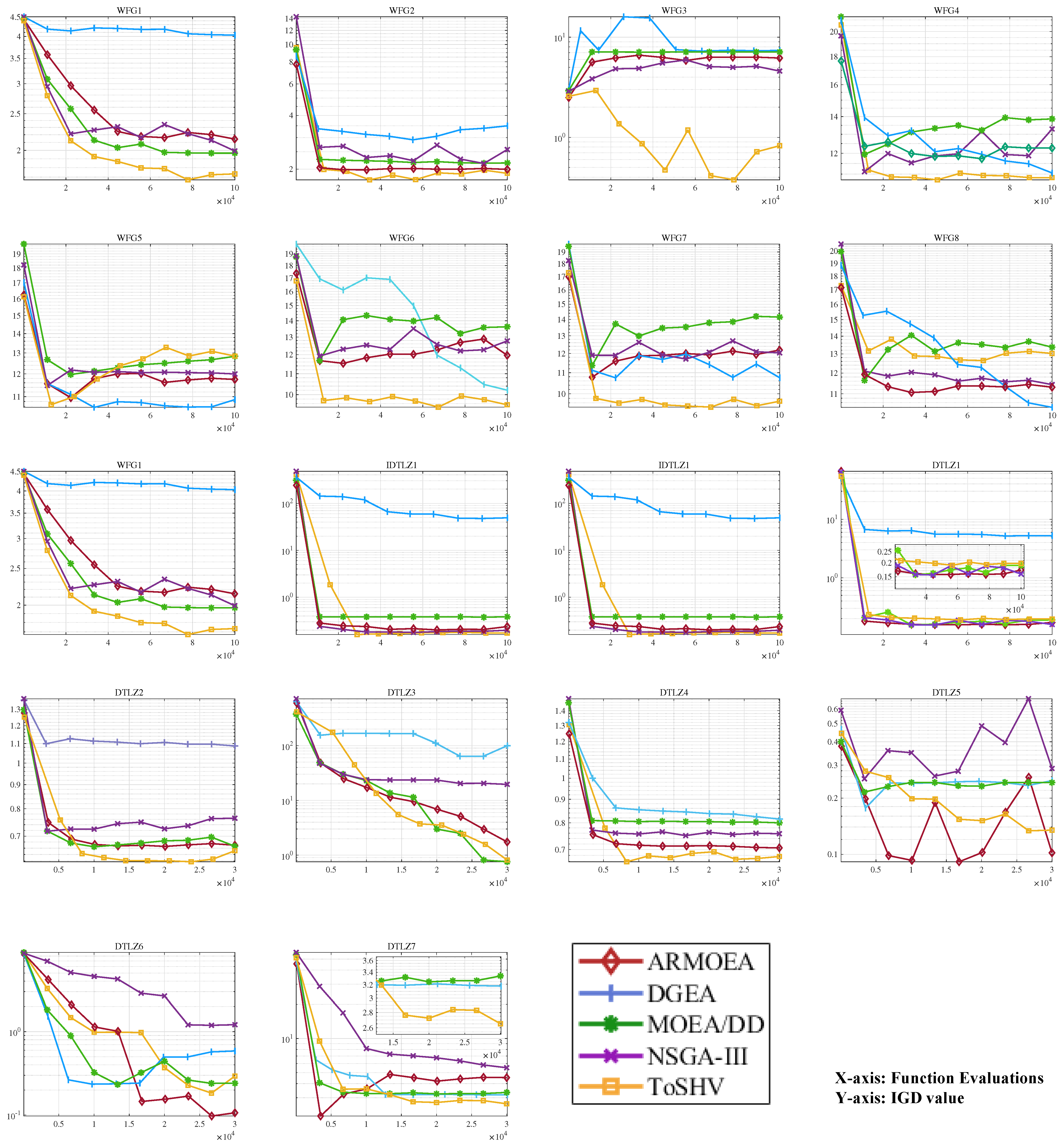
In addition, the solution set distributions of the four algorithms on various test problems in 15 dimensions are shown in Figure 6. It is evident that HypE and SMS-EMOA only explore a small portion of the PF on most problems, indicating poor diversity in their solution sets. On the other hand, both ToSHV and R2HCA-EMOA achieve solution sets that cover a significant portion of the PF, but ToSHV exhibits higher diversity in its solution set. Specifically, on WFG6, R2HCA-EMOA fails to explore the solution space corresponding to objectives 1–5 on the PF, whereas ToSHV successfully explores the PF across most of the objective space. In Figure A3 in Appendix C, we present the distribution of solutions on more problems for 4 hypervolume-based algorithms, including ToSHV.

Figure 6.
The solution distribution of ToSHV and three hypervolume-based EMOAs on 15-dimensional WFG5 and WFG6 problems.
Lastly, we visualize the dynamic evolution of the population hypervolume during the algorithm’s execution, as depicted in Figure 7. On the WFG 1–9 problems, both ToSHV and R2HCA-EMOA stand out by yielding superior outcomes, surpassing the performance of SMS-EMOA and HypE. Notably, ToSHV exhibits notable superiority on WFG4 and WFG5, while R2HCA-EMOA excels on WFG6. Across other WFG problems, the performance of these two algorithms remains comparable. Turning to the DTLZ 1–7 and IDTLZ 1–2 problems, HypE demonstrates commendable search capabilities, and SMS-EMOA, gradual convergence. Meanwhile, ToSHV and R2HCA-EMOA consistently secure the lead on most challenges. While both ToSHV and R2HCA-EMOA exhibit similar performance metrics across various problems, considering ToSHV’s lower runtime compared with R2HCA-EMOA, ToSHV’s comprehensive performance emerges as a strong contender among hypervolume-based EMOAs. At the same time, we also plotted the IGD variations of the population during the running of the algorithm, as shown in Figure A1 in Appendix B.
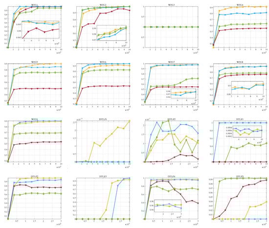

Figure 7.
Hypervolume variations over function evaluations obtained with R2HCA-EMOA, HypE, SMS-EMOA, and ToSHV on WFG 1–9, IDTLZ 1–2, and DTLZ 1–7 problems with 15 objectives.
4.3. Comparison with Other State-of-the-Art EMOAs
In this subsection, we compare ToSHV with four other EMOAs based on different mechanics, namely, AR-MOEA, DGEA, MOEA/DD, and NSGA-III.
Table 3 and Table 4 present the results of the rank-sum tests for hypervolume and IGD, respectively, and the detailed results (means and variances) can be found in Table A5 and Table A6 in Appendix A.2. The results demonstrate that ToSHV outperforms the four comparison algorithms in terms of hypervolume in both test sets. This superiority can be attributed to ToSHV’s specific focus on optimizing the hypervolume, unlike the other algorithms. Regarding IGD, ToSHV still exhibits significant performance compared with the other algorithms. It is worth noting that the IGD results of the proposed algorithm might appear slightly inferior to the hypervolume results. However, this discrepancy is reasonable since the optimal arrangement of the solution set for the hypervolume indicator differs from that of the IGD indicator.
Table 3.
Wilcoxon rank-sum test results for hypervolume obtained with AR-MOEA, DGEA, MOEA/DD, NSGA-III, and ToSHV for 5-, 10-, and 15-objective DTLZ, IDTLZ, and WFG problems.
Table 4.
Wilcoxon rank-sum test results for IGD obtained with AR-MOEA, DGEA, MOEA/DD, NSGA-III, and ToSHV for 5-, 10-, and 15-objective DTLZ, IDTLZ, and WFG problems.
Additionally, we provide an analysis of how the hypervolume of the population obtained with the five algorithms varies with the number of function evaluations across different test problems. Figure 8 clearly illustrates the results. It can be observed that MOEA/DD demonstrates the fastest convergence speed on DTLZ and IDTLZ test problems but that it tends to converge to local optima in certain cases. On the other hand, ToSHV exhibits the best steady-state performance, and it excels in both convergence speed and global search capability. DGEA, however, shows relatively weaker convergence speed and global search ability. In the case of WFG test problems, ToSHV showcases an absolute advantage in terms of convergence speed and search ability. AR-MOEA and NSGA-III yield similar effects and reach steady-state nearly simultaneously. We also plotted the IGD variations of the population during the running of algorithms and put them in Figure A2 in Appendix B.

Figure 8.
Hypervolume variations over function evaluations obtained with AR−MOEA, DGEA, MOEA/DD, NSGA−III, and ToSHV on the 5-objective problems.
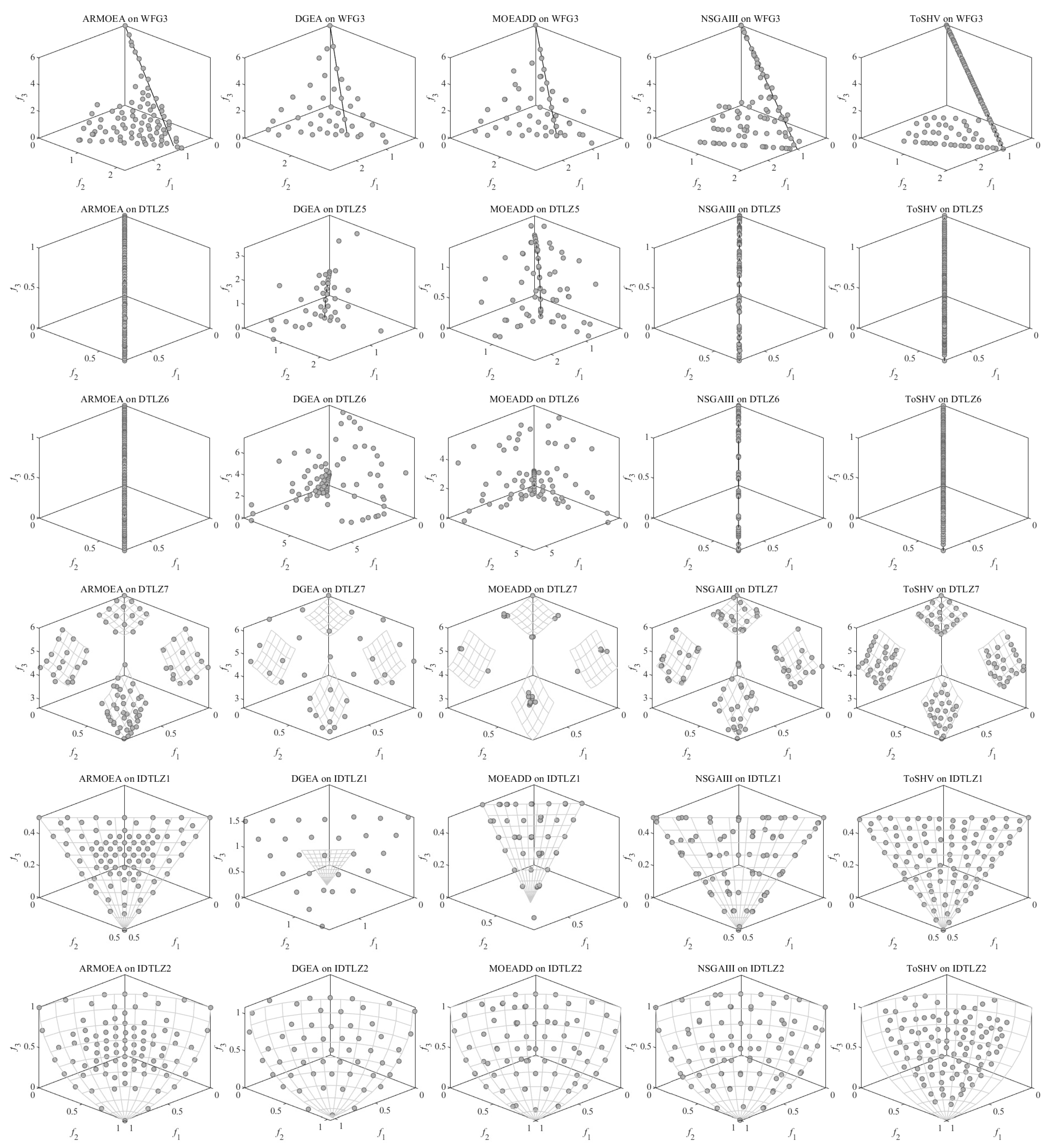
Finally, to assess the search capability of ToSHV on problems with irregular PFs, we conducted experiments using several problem sets specifically designed for this purpose. It is worth noting that we set the number of objectives for these problems to 3, allowing us to observe the spatial distribution of the solutions and evaluate the algorithm’s performance in capturing diverse and non-uniform PFs. Figure 9 illustrates the solution distribution of solutions obtained with ToSHV and four other comparison algorithms on different problem sets. Each row in the figure represents a specific test problem, while each column represents a different algorithm. It is evident that ToSHV demonstrates superior performance on disconnected, degenerated, and inverted PFs. In contrast, decomposition-based algorithms exhibit non-uniform distributions of solutions. For instance, the solutions generated by MOEA/DD on DTLZ7 appear clustered and fail to distribute evenly across the PF. Similarly, on IDTLZ1, the solutions produced by AR-MOEA exhibit a centrally clustered pattern compared with ToSHV. In Figure A4 in Appendix C, we plot the solution distribution of the algorithms on more problems with irregular PFs.

Figure 9.
Distribution of solutions obtained with AR-MOEA, DGEA, MOEA/DD, NSGA-III, and ToSHV on the 3-objective problems.
5. Conclusions
In this paper, we propose a two-stage hypervolume-based evolutionary algorithm designed to tackle MaOPs. The algorithm comprises two stages with distinct evolutionary strategies: a global search stage utilizing the ( + ’) evolutionary strategy and a local search stage employing the ( + 1) evolutionary strategy. To ensure efficient search capabilities across test problems with diverse attributes, we incorporate a mechanism for the mutual conversion of the two stages and develop a fast approximation method for the overall hypervolume contribution. In the experimental section, we compare our proposed algorithm with several state-of-the-art EMOAs. The results demonstrate that our algorithm exhibits competitiveness on the majority of tested problems.
For our future work, we outline three key directions for further exploration. Firstly, we aim to apply the ToSHV algorithm to address practical engineering problems, including UAV marshaling and multi-robot task assignment. By leveraging the strengths of ToSHV, we anticipate achieving effective solutions in these real-world scenarios. Additionally, we plan to enhance the computational efficiency of the ToSHV algorithm by integrating more advanced hypervolume contribution approximation methods. This improvement could allow us to optimize the algorithm’s performance while maintaining its accuracy and effectiveness. By pursuing these avenues of research, we aim to extend the applicability and efficiency of ToSHV in solving complex optimization problems and enable its practical deployment in various engineering domains. Finally, combining ToSHV with some efficient numerical algorithms [34] is also an interesting direction.
Author Contributions
C.W.: conceptualization; methodology; writing—original draft preparation. H.M.: software; validation; formal analysis; writing—review and editing. All authors have read and agreed to the published version of the manuscript.
Funding
This work was partially funded by National Key Research and Development Plan of China (No. 2018AAAOI-01000) and National Natural Science Foundation of China under grant 62076028.
Data Availability Statement
Data are available on request from the authors.
Conflicts of Interest
The authors declare no conflict of interest.
Appendix A. Detailed Numerical Results
Appendix A.1. Detailed Numerical Results with Hypervolume-Based Comparison Algorithms
Table A1.
Statistical results of hypervolume values obtained with R2HCA-EMOA, HypE, SMS-EMOA, and ToSHV on WFG 1–9 problems with 5, 10, 15 objectives.
Table A1.
Statistical results of hypervolume values obtained with R2HCA-EMOA, HypE, SMS-EMOA, and ToSHV on WFG 1–9 problems with 5, 10, 15 objectives.
| Problem | M | D | R2HCAEMOA | HypE | SMSEMOA | ToSHV |
|---|---|---|---|---|---|---|
| 5 | 28 | 9.9236e−1 (5.85e−3) ≈ | 6.1329e−1 (2.81e−2) − | 5.5717e−1 (3.24e−2) − | 9.9410e−1 (6.29e−3) | |
| WFG1 | 10 | 38 | 9.9550e−1 (8.40e−3) ≈ | 6.1330e−1 (3.61e−2) − | 4.5057e−1 (3.57e−2) − | 9.9221e−1 (1.57e−2) |
| 15 | 48 | 9.9739e−1 (1.83e−3) ≈ | 5.5238e−1 (4.49e−2) − | 3.9492e−1 (2.68e−2) − | 9.9788e−1 (1.54e−3) | |
| 5 | 28 | 9.9233e−1 (2.17e−3) ≈ | 9.7595e−1 (8.88e−3) − | 9.5940e−1 (7.08e−3) − | 9.9133e−1 (4.52e−3) | |
| WFG2 | 10 | 39 | 9.9412e−1 (2.16e−3) ≈ | 9.6318e−1 (1.52e−2) − | 9.3567e−1 (1.98e−2) − | 9.9421e−1 (1.78e−3) |
| 15 | 48 | 9.9306e−1 (2.06e−3) ≈ | 9.3237e−1 (4.25e−2) − | 8.6978e−1 (6.41e−2) − | 9.9060e−1 (5.32e−3) | |
| 5 | 28 | 2.2264e−1 (2.48e−2) − | 2.5250e−1 (1.02e−2) + | 2.0621e−1 (1.01e−2) − | 2.3323e−1 (1.91e−2) | |
| WFG3 | 10 | 39 | 3.0686e−2 (3.16e−2) ≈ | 2.5434e−4 (1.39e−3) − | 0.0000e+0 (0.00e+0) − | 2.6352e−2 (2.60e−2) |
| 15 | 48 | 0.0000e+0 (0.00e+0) ≈ | 0.0000e+0 (0.00e+0) ≈ | 0.0000e+0 (0.00e+0) ≈ | 0.0000e+0 (0.00e+0) | |
| 5 | 28 | 7.9131e−1 (1.66e−3) ≈ | 7.2112e−1 (3.68e−2) − | 7.4565e−1 (1.36e−2) − | 7.9066e−1 (2.29e−3) | |
| WFG4 | 10 | 38 | 8.8116e−1 (7.14e−2) ≈ | 6.6518e−1 (4.92e−2) − | 6.4899e−1 (7.07e−2) − | 8.4922e−1 (9.59e−2) |
| 15 | 48 | 9.0337e−1 (4.62e−2) ≈ | 6.3624e−1 (6.44e−2) − | 5.5092e−1 (6.74e−2) − | 8.9830e−1 (4.55e−2) | |
| 5 | 28 | 7.4655e−1 (1.51e−3) ≈ | 7.3780e−1 (1.91e−3) − | 7.2132e−1 (3.55e−3) − | 7.4652e−1 (1.13e−3) | |
| WFG5 | 10 | 38 | 8.7933e−1 (2.79e−2) ≈ | 7.5362e−1 (3.47e−2) − | 5.4073e−1 (5.84e−2) − | 8.7660e−1 (5.56e−2) |
| 15 | 48 | 8.5189e−1 (4.48e−2) ≈ | 7.2676e−1 (2.15e−2) − | 4.8707e−1 (1.28e−2) − | 8.5974e−1 (8.11e−2) | |
| 5 | 28 | 7.6007e−1 (4.71e−3) ≈ | 7.4204e−1 (6.92e−3) − | 7.1978e−1 (6.89e−3) − | 7.5971e−1 (5.73e−3) | |
| WFG6 | 10 | 38 | 8.9598e−1 (3.75e−2) ≈ | 7.3776e−1 (3.93e−2) − | 7.2966e−1 (4.88e−2) − | 8.9481e−1 (5.14e−2) |
| 15 | 48 | 8.7892e−1 (5.89e−2) ≈ | 7.1818e−1 (3.87e−2) − | 6.4681e−1 (5.61e−2) − | 8.9766e−1 (3.76e−2) | |
| 5 | 28 | 7.3790e−1 (2.36e−3) ≈ | 7.0263e−1 (4.83e−3) − | 6.7269e−1 (5.40e−3) − | 7.3779e−1 (4.47e−3) | |
| WFG8 | 10 | 38 | 8.4406e−1 (3.22e−2) ≈ | 7.5125e−1 (3.54e−2) − | 7.1770e−1 (5.06e−2) − | 8.3619e−1 (3.23e−2) |
| 15 | 48 | 8.6609e−1 (3.34e−2) ≈ | 7.3784e−1 (4.69e−2) − | 6.8280e−1 (6.94e−2) − | 8.6085e−1 (5.46e−2) | |
| 5 | 28 | 7.9587e−1 (1.17e−3) ≈ | 7.8108e−1 (9.04e−3) − | 7.5813e−1 (3.20e−3) − | 7.9605e−1 (1.05e−3) | |
| WFG7 | 10 | 38 | 9.2783e−1 (5.69e−2) ≈ | 7.4631e−1 (4.37e−2) − | 7.3517e−1 (5.83e−2) − | 9.3566e−1 (4.24e−2) |
| 15 | 48 | 9.4867e−1 (3.58e−2) ≈ | 7.2063e−1 (6.01e−2) − | 6.2362e−1 (8.61e−2) − | 9.3456e−1 (5.27e−2) | |
| 5 | 28 | 7.6880e−1 (1.31e−2) ≈ | 7.2809e−1 (2.63e−2) − | 7.2267e−1 (1.22e−2) − | 7.6575e−1 (2.08e−2) | |
| WFG9 | 10 | 38 | 8.6288e−1 (7.56e−2) ≈ | 6.9209e−1 (4.75e−2) − | 5.1399e−1 (6.47e−2) − | 8.4341e−1 (1.32e−1) |
| 15 | 48 | 8.4314e−1 (6.72e−2) ≈ | 7.0257e−1 (4.23e−2) − | 4.6765e−1 (4.25e−2) − | 8.5875e−1 (5.59e−2) | |
| 0/1/26 | 1/25/1 | 0/26/1 | ||||
Table A2.
Statistical results of hypervolume values obtained with R2HCA-EMOA, HypE, SMS-EMOA, and ToSHV on IDTLZ 1–2 and DTLZ 1–7 problems with 5, 10, 15 objectives.
Table A2.
Statistical results of hypervolume values obtained with R2HCA-EMOA, HypE, SMS-EMOA, and ToSHV on IDTLZ 1–2 and DTLZ 1–7 problems with 5, 10, 15 objectives.
| Problem | M | D | R2HCAEMOA | HypE | SMSEMOA | ToSHV |
|---|---|---|---|---|---|---|
| 5 | 9 | 1.0082e−2 (1.40e−4) ≈ | 1.3900e−3 (2.07e−4) − | 8.8477e−3 (3.44e−4) − | 1.0005e−2 (1.82e−4) | |
| IDTLZ1 | 10 | 14 | 1.7745e−7 (1.64e−7) ≈ | 2.4305e−8 (9.44e−8) − | 2.2202e−7 (4.34e−8) ≈ | 1.7722e−7 (2.45e−7) |
| 15 | 19 | 0.0000e+0 (0.00e+0) ≈ | 3.1290e−14 (8.12e−14) + | 2.0477e−12 (4.54e−13) + | 0.0000e+0 (0.00e+0) | |
| 5 | 14 | 1.2533e−1 (5.93e−4) ≈ | 9.0413e−2 (2.86e−3) − | 1.1019e−1 (1.96e−3) − | 1.2551e−1 (7.30e−4) | |
| IDTLZ2 | 10 | 19 | 4.3957e−4 (1.02e−5) ≈ | 1.1848e−4 (1.58e−5) − | 2.4476e−4 (3.19e−5) − | 4.3611e−4 (1.54e−5) |
| 15 | 24 | 2.0470e−7 (4.63e−8) ≈ | 6.1836e−8 (6.15e−8) − | 4.2764e−8 (2.48e−8) − | 1.8224e−7 (3.75e−8) | |
| 5 | 9 | 9.7166e−1 (1.17e−3) ≈ | 5.7295e−1 (1.07e−1) − | 8.2526e−1 (1.49e−1) − | 9.7152e−1 (2.41e−3) | |
| DTLZ1 | 10 | 14 | 9.9755e−1 (2.00e−3) ≈ | 4.9493e−1 (8.97e−2) − | 1.1125e−1 (2.64e−1) − | 9.9571e−1 (1.20e−2) |
| 15 | 19 | 9.9887e−1 (1.07e−3) ≈ | 4.8902e−1 (8.14e−2) − | 2.1743e−1 (3.41e−1) − | 9.9899e−1 (1.14e−3) | |
| 5 | 14 | 7.9806e−1 (8.46e−4) − | 7.0972e−1 (1.75e−2) − | 7.7601e−1 (3.06e−3) − | 7.9860e−1 (8.46e−4) | |
| DTLZ2 | 10 | 19 | 9.5413e−1 (9.04e−4) ≈ | 7.1060e−1 (3.41e−2) − | 8.0662e−1 (3.32e−2) − | 9.4969e−1 (2.32e−2) |
| 15 | 24 | 9.5541e−1 (5.40e−2) ≈ | 7.0265e−1 (4.59e−2) − | 7.7388e−1 (4.40e−2) − | 9.5133e−1 (5.19e−2) | |
| 5 | 14 | 5.9639e−1 (2.81e−1) + | 1.1597e−1 (1.72e−1) ≈ | 6.5278e−3 (3.58e−2) − | 2.2760e−1 (3.08e−1) | |
| DTLZ3 | 10 | 19 | 6.1666e−1 (4.15e−1) − | 2.1371e−2 (8.17e−2) − | 0.0000e+0 (0.00e+0) − | 7.7102e−1 (3.36e−1) |
| 15 | 24 | 4.7133e−1 (4.31e−1) − | 0.0000e+0 (0.00e+0) − | 0.0000e+0 (0.00e+0) − | 7.2421e−1 (4.07e−1) | |
| 5 | 14 | 7.3533e−1 (6.63e−2) ≈ | 5.8997e−1 (1.33e−1) − | 6.7247e−1 (1.15e−1) − | 7.6889e−1 (5.65e−2) | |
| DTLZ4 | 10 | 19 | 9.1325e−1 (4.62e−2) ≈ | 7.4072e−1 (6.53e−2) − | 8.4724e−1 (8.31e−2) − | 8.9894e−1 (4.12e−2) |
| 15 | 24 | 9.5633e−1 (3.10e−2) ≈ | 7.5312e−1 (4.20e−2) − | 3.4193e−1 (3.29e−1) − | 9.4716e−1 (2.21e−2) | |
| 5 | 14 | 1.1735e−1 (6.70e−3) ≈ | 1.2366e−1 (1.23e−3) + | 1.1536e−1 (1.76e−3) − | 1.1774e−1 (6.62e−3) | |
| DTLZ5 | 10 | 19 | 5.7484e−2 (1.93e−2) ≈ | 9.6749e−2 (7.24e−4) + | 8.8767e−2 (2.28e−3) + | 5.2176e−2 (3.11e−2) |
| 15 | 24 | 4.1738e−2 (3.10e−2) ≈ | 9.2463e−2 (4.57e−4) + | 8.4195e−2 (6.03e−3) + | 5.3533e−2 (2.82e−2) | |
| 5 | 14 | 1.1200e−1 (9.04e−3) ≈ | 9.9899e−2 (6.45e−3) − | 3.4014e−2 (4.30e−2) − | 1.1395e−1 (8.51e−3) | |
| DTLZ6 | 10 | 19 | 8.4916e−2 (2.34e−2) ≈ | 9.2014e−2 (1.64e−3) ≈ | 0.0000e+0 (0.00e+0) − | 7.6666e−2 (3.23e−2) |
| 15 | 24 | 5.8723e−2 (4.26e−2) ≈ | 9.0885e−2 (2.51e−4) ≈ | 0.0000e+0 (0.00e+0) − | 6.3795e−2 (3.88e−2) | |
| 5 | 24 | 2.5599e−1 (1.88e−2) − | 1.8670e−1 (7.09e−3) − | 2.1411e−1 (2.57e−2) − | 2.7309e−1 (6.38e−3) | |
| DTLZ7 | 10 | 29 | 1.7195e−1 (1.08e−2) ≈ | 1.2924e−1 (6.05e−3) − | 1.3001e−1 (6.52e−3) − | 1.7002e−1 (1.05e−2) |
| 15 | 34 | 1.3330e−1 (2.17e−2) ≈ | 1.1135e−1 (3.94e−3) − | 1.0230e−1 (9.71e−3) − | 1.3182e−1 (2.15e−2) | |
| 1/4/22 | 4/20/3 | 3/23/1 | ||||
Table A3.
Statistical results of IGD values obtained with R2HCA-EMOA, HypE, SMS-EMOA, and ToSHV on WFG 1–9 problems with 5, 10, 15 objectives.
Table A3.
Statistical results of IGD values obtained with R2HCA-EMOA, HypE, SMS-EMOA, and ToSHV on WFG 1–9 problems with 5, 10, 15 objectives.
| Problem | M | D | R2HCAEMOA | HypE | SMSEMOA | ToSHV |
|---|---|---|---|---|---|---|
| 5 | 28 | 4.7921e−1 (1.55e−2) ≈ | 1.4736e+0 (8.43e−2) − | 1.2593e+0 (7.79e−2) − | 4.8063e−1 (1.60e−2) | |
| WFG1 | 10 | 38 | 1.1811e+0 (9.69e−2) ≈ | 2.0732e+0 (3.64e−2) − | 2.2049e+0 (8.58e−2) − | 1.1823e+0 (1.05e−1) |
| 15 | 48 | 1.6867e+0 (6.88e−2) ≈ | 2.7212e+0 (5.69e−2) − | 3.1343e+0 (1.05e−1) − | 1.7206e+0 (8.42e−2) | |
| 5 | 28 | 6.0579e−1 (1.21e−1) ≈ | 6.1442e−1 (3.68e−2) + | 9.4449e−1 (7.98e−2) − | 6.1627e−1 (1.30e−1) | |
| WFG2 | 10 | 39 | 1.4250e+0 (1.66e−1) ≈ | 1.3894e+0 (1.14e−1) ≈ | 2.6286e+0 (4.76e−1) − | 1.4086e+0 (1.90e−1) |
| 15 | 48 | 2.0112e+0 (1.18e−1) ≈ | 2.8447e+0 (1.03e+0) − | 5.9360e+0 (1.33e+0) − | 2.0259e+0 (1.66e−1) | |
| 5 | 28 | 2.1274e−1 (6.32e−2) ≈ | 9.1455e−2 (1.52e−2) + | 4.6214e−1 (2.88e−1) − | 2.2207e−1 (6.53e−2) | |
| WFG3 | 10 | 39 | 8.7369e−1 (2.29e+0) ≈ | 2.2119e−1 (4.72e−2) ≈ | 2.9874e+0 (2.12e+0) − | 4.2759e−1 (1.13e+0) |
| 15 | 48 | 5.5974e−1 (3.08e−1) ≈ | 4.0134e−1 (6.50e−2) + | 6.0839e+0 (2.18e+0) − | 8.9388e−1 (1.21e+0) | |
| 5 | 28 | 1.4620e+0 (3.56e−2) ≈ | 1.6297e+0 (1.41e−1) − | 1.3748e+0 (5.10e−2) + | 1.4557e+0 (2.59e−2) | |
| WFG4 | 10 | 38 | 6.0009e+0 (7.04e−1) ≈ | 9.5151e+0 (8.51e−1) − | 9.7522e+0 (1.28e+0) − | 6.3055e+0 (1.35e+0) |
| 15 | 48 | 1.0835e+1 (1.36e+0) ≈ | 1.9593e+1 (1.44e+0) − | 2.1029e+1 (1.40e+0) − | 1.1085e+1 (1.21e+0) | |
| 5 | 28 | 1.4338e+0 (3.01e−2) ≈ | 1.5523e+0 (3.54e−2) − | 1.3755e+0 (2.62e−2) + | 1.4306e+0 (3.09e−2) | |
| WFG5 | 10 | 38 | 5.5943e+0 (2.15e−1) ≈ | 6.7119e+0 (6.22e−1) − | 1.0700e+1 (1.14e+0) − | 5.7028e+0 (7.31e−1) |
| 15 | 48 | 1.0445e+1 (1.24e+0) ≈ | 1.5402e+1 (9.10e−1) − | 2.1535e+1 (6.58e−1) − | 1.0581e+1 (2.45e+0) | |
| 5 | 28 | 1.4508e+0 (3.01e−2) ≈ | 1.5525e+0 (3.34e−2) − | 1.4193e+0 (3.79e−2) + | 1.4552e+0 (4.33e−2) | |
| WFG6 | 10 | 38 | 5.7099e+0 (3.73e−1) ≈ | 7.5548e+0 (8.13e−1) − | 7.8373e+0 (1.02e+0) − | 5.7405e+0 (4.92e−1) |
| 15 | 48 | 1.0659e+1 (1.82e+0) ≈ | 1.6686e+1 (1.38e+0) − | 1.8531e+1 (1.56e+0) − | 1.0179e+1 (8.40e−1) | |
| 5 | 28 | 1.4747e+0 (3.49e−2) ≈ | 1.5813e+0 (4.15e−2) − | 1.4482e+0 (3.12e−2) + | 1.4817e+0 (3.00e−2) | |
| WFG7 | 10 | 38 | 5.8212e+0 (5.22e−1) ≈ | 8.1365e+0 (9.09e−1) − | 8.3765e+0 (1.04e+0) − | 5.7466e+0 (4.04e−1) |
| 15 | 48 | 9.9880e+0 (8.12e−1) ≈ | 1.7738e+1 (1.64e+0) − | 1.9754e+1 (2.07e+0) − | 1.0441e+1 (1.25e+0) | |
| 5 | 28 | 1.3607e+0 (3.02e−2) ≈ | 1.5179e+0 (2.66e−2) − | 1.3874e+0 (3.29e−2) − | 1.3663e+0 (4.21e−2) | |
| WFG8 | 10 | 38 | 5.9871e+0 (7.07e−1) ≈ | 7.5353e+0 (6.03e−1) − | 8.2559e+0 (1.09e+0) − | 6.1673e+0 (7.18e−1) |
| 15 | 48 | 1.1703e+1 (1.17e+0) ≈ | 1.6665e+1 (1.60e+0) − | 1.7933e+1 (1.93e+0) − | 1.1595e+1 (1.66e+0) | |
| 5 | 28 | 1.4375e+0 (3.85e−2) ≈ | 1.4890e+0 (6.88e−2) − | 1.3728e+0 (2.91e−2) + | 1.4323e+0 (4.03e−2) | |
| WFG9 | 10 | 38 | 5.9441e+0 (1.19e+0) ≈ | 7.6574e+0 (8.28e−1) − | 1.1223e+1 (9.84e−1) − | 6.2827e+0 (2.11e+0) |
| 15 | 48 | 1.1474e+1 (2.44e+0) ≈ | 1.6289e+1 (1.22e+0) − | 2.1988e+1 (8.69e−1) − | 1.1228e+1 (1.95e+0) | |
| 0/0/27 | 3/22/2 | 5/22/0 | ||||
Table A4.
Statistical results of IGD values obtained with R2HCA-EMOA, HypE, SMS-EMOA, and ToSHV on IDTLZ 1–2 and DTLZ 1–7 problems with 5, 10, 15 objectives.
Table A4.
Statistical results of IGD values obtained with R2HCA-EMOA, HypE, SMS-EMOA, and ToSHV on IDTLZ 1–2 and DTLZ 1–7 problems with 5, 10, 15 objectives.
| Problem | M | D | R2HCAEMOA | HypE | SMSEMOA | ToSHV |
|---|---|---|---|---|---|---|
| 5 | 9 | 6.6209e−2 (5.56e−4) ≈ | 2.2770e−1 (1.30e−2) − | 7.6514e−2 (2.83e−3) − | 6.6415e−2 (6.62e−4) | |
| IDTLZ1 | 10 | 14 | 1.3084e−1 (2.03e−3) ≈ | 2.9827e−1 (1.54e−2) − | 1.6223e−1 (8.24e−3) − | 1.3038e−1 (1.84e−3) |
| 15 | 19 | 1.7236e−1 (5.02e−3) ≈ | 3.1168e−1 (4.22e−2) − | 1.8756e−1 (5.81e−3) − | 1.7302e−1 (5.73e−3) | |
| 5 | 14 | 2.8427e−1 (1.02e−2) ≈ | 1.9886e−1 (1.69e−3) + | 3.4355e−1 (1.63e−2) − | 2.8189e−1 (8.59e−3) | |
| IDTLZ2 | 10 | 19 | 5.6360e−1 (1.27e−2) ≈ | 4.3690e−1 (2.57e−3) + | 6.2789e−1 (1.65e−2) − | 5.6172e−1 (9.49e−3) |
| 15 | 24 | 6.5531e−1 (1.10e−2) ≈ | 5.6942e−1 (3.18e−3) + | 7.5324e−1 (2.06e−2) − | 6.5520e−1 (1.75e−2) | |
| 5 | 9 | 6.7188e−2 (8.20e−4) ≈ | 2.6606e−1 (4.64e−2) − | 1.3500e−1 (5.25e−2) − | 6.7302e−2 (1.72e−3) | |
| DTLZ1 | 10 | 14 | 1.4211e−1 (9.46e−3) ≈ | 3.6931e−1 (3.19e−2) − | 3.7086e+0 (3.11e+0) − | 1.4080e−1 (1.29e−2) |
| 15 | 19 | 1.8108e−1 (1.13e−2) ≈ | 3.9195e−1 (2.79e−2) − | 1.7573e+0 (2.28e+0) − | 1.7824e−1 (1.13e−2) | |
| 5 | 14 | 2.4397e−1 (3.54e−3) ≈ | 3.5939e−1 (1.59e−2) − | 2.4036e−1 (4.28e−3) + | 2.4355e−1 (3.69e−3) | |
| DTLZ2 | 10 | 19 | 4.9889e−1 (1.85e−3) ≈ | 7.9163e−1 (3.78e−2) − | 7.3465e−1 (5.05e−2) − | 5.0711e−1 (4.12e−2) |
| 15 | 24 | 6.6106e−1 (8.10e−2) ≈ | 9.5061e−1 (3.97e−2) − | 9.5251e−1 (4.15e−2) − | 6.7513e−1 (8.87e−2) | |
| 5 | 14 | 3.9625e−1 (2.98e−1) + | 1.6225e+0 (1.28e+0) − | 4.6978e+0 (2.45e+0) − | 8.8943e−1 (5.07e−1) | |
| DTLZ3 | 10 | 19 | 7.8395e−1 (4.23e−1) − | 2.5177e+0 (1.33e+0) − | 8.8989e+1 (2.61e+1) − | 6.3322e−1 (2.63e−1) |
| 15 | 24 | 1.2437e+0 (7.99e−1) − | 3.9161e+0 (2.32e+0) − | 8.7311e+1 (2.26e+1) − | 8.2527e−1 (3.19e−1) | |
| 5 | 14 | 3.6542e−1 (1.19e−1) ≈ | 5.7025e−1 (1.67e−1) − | 4.2838e−1 (1.83e−1) − | 3.0286e−1 (1.01e−1) | |
| DTLZ4 | 10 | 19 | 5.7122e−1 (5.53e−2) + | 7.7531e−1 (6.32e−2) − | 6.1911e−1 (8.11e−2) ≈ | 6.0759e−1 (6.41e−2) |
| 15 | 24 | 6.6986e−1 (4.13e−2) + | 8.9130e−1 (3.42e−2) − | 1.0887e+0 (2.28e−1) − | 6.9633e−1 (3.64e−2) | |
| 5 | 14 | 4.9856e−2 (1.89e−2) ≈ | 3.5084e−2 (4.43e−3) + | 5.1959e−2 (1.59e−2) ≈ | 5.2227e−2 (1.87e−2) | |
| DTLZ5 | 10 | 19 | 3.3896e−1 (1.83e−1) ≈ | 5.3620e−2 (6.46e−3) + | 1.6327e−1 (5.11e−2) + | 3.1738e−1 (1.64e−1) |
| 15 | 24 | 4.1375e−1 (2.45e−1) ≈ | 6.3660e−2 (1.15e−2) + | 2.0957e−1 (4.16e−2) ≈ | 3.4433e−1 (2.23e−1) | |
| 5 | 14 | 8.3122e−2 (3.70e−2) ≈ | 2.0500e−1 (5.36e−2) − | 6.1085e−1 (4.65e−1) − | 7.1247e−2 (3.33e−2) | |
| DTLZ6 | 10 | 19 | 2.5767e−1 (1.78e−1) ≈ | 1.7085e−1 (6.39e−2) ≈ | 2.2206e+0 (5.75e−1) − | 2.4048e−1 (2.28e−1) |
| 15 | 24 | 5.6279e−1 (6.68e−1) ≈ | 2.7975e−1 (7.56e−2) ≈ | 2.6570e+0 (6.58e−1) − | 4.6759e−1 (5.42e−1) | |
| 5 | 24 | 5.2304e−1 (2.34e−1) − | 1.7698e+0 (1.01e−1) − | 9.7422e−1 (4.53e−1) − | 3.4222e−1 (4.65e−2) | |
| DTLZ7 | 10 | 29 | 2.0275e+0 (6.81e−1) ≈ | 5.4616e+0 (2.17e−1) − | 5.5231e+0 (2.33e−1) − | 2.1016e+0 (7.98e−1) |
| 15 | 34 | 5.4889e+0 (1.76e+0) ≈ | 1.1228e+1 (1.94e−1) − | 1.1581e+1 (3.69e−1) − | 5.2840e+0 (1.43e+0) | |
| 3/3/21 | 6/19/2 | 1/23/3 | ||||
Appendix A.2. Detailed Numerical Results with State-of-the-Art Comparison Algorithms
Table A5.
Statistical results of hypervolume results (mean and standard deviation) obtained with AR-MOEA, DGEA, MOEA/DD, NSGA-III, and ToSHV on WFG 1–9, IDTLZ 1–2, and DTLZ 1–7 problems with 5, 10, 15 objectives.
Table A5.
Statistical results of hypervolume results (mean and standard deviation) obtained with AR-MOEA, DGEA, MOEA/DD, NSGA-III, and ToSHV on WFG 1–9, IDTLZ 1–2, and DTLZ 1–7 problems with 5, 10, 15 objectives.
| Problem | M | D | AR-MOEA | DGEA | MOEA/DD | NSGA-III | ToSHV |
|---|---|---|---|---|---|---|---|
| 5 | 28 | 9.7126e−1 (1.92e−2) − | 3.1115e−1 (1.55e−2) − | 9.1157e−1 (2.71e−2) − | 9.5567e−1 (1.78e−2) − | 9.9410e−1 (6.29e−3) | |
| WFG1 | 10 | 38 | 9.3260e−1 (3.85e−2) − | 2.4109e−1 (1.22e−2) − | 9.6551e−1 (2.75e−2) − | 9.4938e−1 (3.83e−2) − | 9.9221e−1 (1.57e−2) |
| 15 | 48 | 4.2115e−1 (3.32e−2) − | 1.9869e−1 (5.85e−3) − | 9.4786e−1 (1.19e−1) − | 9.9461e−1 (1.23e−2) − | 9.9788e−1 (1.54e−3) | |
| 5 | 28 | 9.9059e−1 (2.22e−3) − | 8.1892e−1 (3.26e−2) − | 9.7092e−1 (5.37e−3) − | 9.8976e−1 (2.49e−3) − | 9.9133e−1 (4.52e−3) | |
| WFG2 | 10 | 39 | 9.8082e−1 (7.80e−3) − | 6.4632e−1 (8.47e−2) − | 8.9818e−1 (2.21e−2) − | 9.8105e−1 (9.85e−3) − | 9.9421e−1 (1.78e−3) |
| 15 | 48 | 8.5822e−1 (3.06e−2) − | 6.1439e−1 (1.02e−1) − | 8.0380e−1 (4.28e−2) − | 8.8490e−1 (3.76e−2) − | 9.9060e−1 (5.32e−3) | |
| 5 | 28 | 7.1812e−2 (1.48e−2) − | 8.7225e−4 (3.21e−3) − | 5.5634e−2 (2.23e−2) − | 1.0022e−1 (2.80e−2) − | 2.3323e−1 (1.91e−2) | |
| WFG3 | 10 | 39 | 0.0000e+0 (0.00e+0) − | 0.0000e+0 (0.00e+0) − | 0.0000e+0 (0.00e+0) − | 0.0000e+0 (0.00e+0) − | 2.6352e−2 (2.60e−2) |
| 15 | 48 | 0.0000e+0 (0.00e+0) ≈ | 0.0000e+0 (0.00e+0) ≈ | 0.0000e+0 (0.00e+0) ≈ | 0.0000e+0 (0.00e+0) ≈ | 0.0000e+0 (0.00e+0) | |
| 5 | 28 | 7.6149e−1 (1.64e−3) − | 5.2382e−1 (2.98e−2) − | 7.1444e−1 (7.22e−3) − | 7.5840e−1 (2.01e−2) − | 7.9066e−1 (2.29e−3) | |
| WFG4 | 10 | 38 | 9.2754e−1 (2.20e−3) + | 3.5055e−1 (5.99e−2) − | 5.6273e−1 (5.61e−2) − | 9.1728e−1 (1.75e−2) + | 8.4922e−1 (9.59e−2) |
| 15 | 48 | 6.2056e−1 (5.49e−2) − | 2.8553e−1 (4.83e−2) − | 4.3155e−1 (4.02e−2) − | 7.4685e−1 (3.59e−2) − | 8.9830e−1 (4.55e−2) | |
| 5 | 28 | 7.2324e−1 (5.30e−4) − | 6.3025e−1 (2.14e−2) − | 6.9530e−1 (2.81e−3) − | 7.2348e−1 (4.00e−4) − | 7.4652e−1 (1.13e−3) | |
| WFG5 | 10 | 38 | 8.7420e−1 (6.37e−4) − | 4.2332e−1 (8.40e−2) − | 6.3706e−1 (2.51e−2) − | 8.7295e−1 (8.04e−3) − | 8.7660e−1 (5.56e−2) |
| 15 | 48 | 3.5966e−1 (1.21e−1) − | 2.8883e−1 (4.07e−2) − | 4.6214e−1 (2.05e−2) − | 6.9985e−1 (2.27e−2) − | 8.5974e−1 (8.11e−2) | |
| 5 | 28 | 7.3020e−1 (7.03e−3) − | 6.5273e−1 (4.27e−3) − | 6.8754e−1 (1.02e−2) − | 7.3140e−1 (4.87e−3) − | 7.5971e−1 (5.73e−3) | |
| WFG6 | 10 | 38 | 8.9602e−1 (6.36e−3) + | 6.9973e−1 (4.68e−2) − | 5.5540e−1 (2.49e−2) − | 8.9432e−1 (1.50e−2) − | 8.9481e−1 (5.14e−2) |
| 15 | 48 | 4.5323e−1 (1.04e−1) − | 6.9645e−1 (1.61e−2) − | 2.9267e−1 (5.79e−2) − | 7.1870e−1 (1.70e−2) − | 8.9766e−1 (3.76e−2) | |
| 5 | 28 | 7.6197e−1 (2.40e−3) − | 4.6868e−1 (1.73e−2) − | 7.2135e−1 (8.56e−3) − | 7.6740e−1 (1.19e−3) − | 7.9605e−1 (1.05e−3) | |
| WFG7 | 10 | 38 | 9.3636e−1 (1.98e−3) + | 3.7638e−1 (4.84e−2) − | 5.7901e−1 (4.32e−2) − | 9.3280e−1 (1.62e−2) − | 9.3566e−1 (4.24e−2) |
| 15 | 48 | 5.1858e−1 (9.92e−2) − | 2.9994e−1 (2.21e−2) − | 3.9761e−1 (6.55e−2) − | 7.6010e−1 (1.52e−2) − | 9.3456e−1 (5.27e−2) | |
| 5 | 28 | 7.1036e−1 (2.46e−3) − | 3.8569e−1 (2.59e−2) − | 6.3694e−1 (1.13e−2) − | 7.0976e−1 (2.63e−3) − | 7.3779e−1 (4.47e−3) | |
| WFG8 | 10 | 38 | 8.6279e−1 (4.84e−3) + | 3.2164e−1 (9.53e−2) − | 4.8639e−1 (5.91e−2) − | 8.4964e−1 (1.41e−2) ≈ | 8.3619e−1 (3.23e−2) |
| 15 | 48 | 4.9627e−1 (9.38e−2) − | 3.8609e−1 (8.65e−2) − | 1.0305e−1 (6.99e−2) − | 6.2544e−1 (1.32e−2) − | 8.6085e−1 (5.46e−2) | |
| 5 | 28 | 6.7283e−1 (1.32e−2) − | 5.7753e−1 (2.77e−2) − | 6.3257e−1 (1.84e−2) − | 6.7672e−1 (2.43e−2) − | 7.6575e−1 (2.08e−2) | |
| WFG9 | 10 | 38 | 7.8278e−1 (3.40e−2) − | 5.6538e−1 (6.11e−2) − | 5.4063e−1 (5.02e−2) − | 7.8573e−1 (2.70e−2) − | 8.4341e−1 (1.32e−1) |
| 15 | 48 | 2.6588e−1 (1.06e−1) − | 3.7467e−1 (8.73e−2) − | 3.0913e−1 (1.06e−1) − | 5.3384e−1 (6.41e−2) − | 8.5875e−1 (5.59e−2) | |
| 5 | 9 | 8.5666e−3 (2.80e−4) − | 1.9802e−4 (4.30e−4) − | 3.8258e−3 (4.90e−4) − | 6.0578e−3 (5.32e−4) − | 1.0005e−2 (1.82e−4) | |
| IDTLZ1 | 10 | 14 | 1.2365e−7 (2.64e−7) ≈ | 7.0335e−10 (1.23e−9) ≈ | 4.6071e−9 (3.06e−9) ≈ | 2.1689e−7 (3.43e−8) ≈ | 1.7722e−7 (2.45e−7) |
| 15 | 19 | 1.8042e−13 (1.40e−13) + | 7.2410e−17 (3.71e−16) + | 1.5570e−14 (6.88e−15) + | 1.3394e−12 (4.13e−13) + | 0.0000e+0 (0.00e+0) | |
| 5 | 14 | 8.5063e−2 (3.05e−3) − | 3.6242e−2 (8.43e−3) − | 2.4224e−2 (8.10e−3) − | 5.6260e−2 (5.72e−3) − | 1.2551e−1 (7.30e−4) | |
| IDTLZ2 | 10 | 19 | 1.8593e−4 (2.68e−5) − | 1.3548e−5 (1.05e−5) − | 3.0184e−5 (1.13e−5) − | 1.6576e−4 (1.06e−5) − | 4.3611e−4 (1.54e−5) |
| 15 | 24 | 7.2514e−8 (3.72e−8) − | 5.2622e−12 (2.16e−11) − | 8.0253e−10 (1.10e−9) − | 1.0323e−7 (4.13e−9) − | 1.8224e−7 (3.75e−8) | |
| 5 | 9 | 9.0779e−1 (2.02e−1) − | 7.7214e−2 (2.34e−1) − | 9.7067e−1 (2.37e−4) − | 9.6978e−1 (4.54e−3) − | 9.7152e−1 (2.41e−3) | |
| DTLZ1 | 10 | 14 | 7.3662e−1 (3.80e−1) − | 4.0523e−2 (1.80e−1) − | 9.9695e−1 (1.63e−4) + | 9.8805e−1 (3.14e−2) − | 9.9571e−1 (1.20e−2) |
| 15 | 19 | 9.4045e−1 (1.33e−2) − | 4.8245e−2 (1.17e−1) − | 7.9166e−1 (2.85e−2) − | 7.4054e−1 (7.04e−2) − | 9.9899e−1 (1.14e−3) | |
| 5 | 14 | 7.7169e−1 (6.87e−4) − | 5.7848e−1 (3.71e−2) − | 7.7395e−1 (4.33e−4) − | 7.7383e−1 (4.79e−4) − | 7.9860e−1 (8.46e−4) | |
| DTLZ2 | 10 | 19 | 9.3661e−1 (1.43e−3) − | 4.8331e−1 (7.77e−2) − | 9.3805e−1 (3.11e−3) − | 9.1579e−1 (3.11e−2) − | 9.4969e−1 (2.32e−2) |
| 15 | 24 | 7.1506e−1 (2.69e−2) − | 1.5984e−1 (6.06e−2) − | 6.1266e−1 (2.71e−2) − | 7.2885e−1 (2.31e−2) − | 9.5133e−1 (5.19e−2) | |
| 5 | 14 | 0.0000e+0 (0.00e+0) − | 0.0000e+0 (0.00e+0) − | 1.1634e−1 (2.16e−1) ≈ | 1.0019e−2 (4.29e−2) − | 2.2760e−1 (3.08e−1) | |
| DTLZ3 | 10 | 19 | 0.0000e+0 (0.00e+0) − | 0.0000e+0 (0.00e+0) − | 2.2336e−1 (3.66e−1) − | 0.0000e+0 (0.00e+0) − | 7.7102e−1 (3.36e−1) |
| 15 | 24 | 1.0623e−1 (2.19e−1) − | 0.0000e+0 (0.00e+0) − | 1.6428e−1 (1.49e−1) − | 0.0000e+0 (0.00e+0) − | 7.2421e−1 (4.07e−1) | |
| 5 | 14 | 7.5189e−1 (5.00e−2) − | 5.7783e−1 (6.05e−2) − | 7.6250e−1 (3.61e−2) − | 7.1820e−1 (7.12e−2) − | 7.6889e−1 (5.65e−2) | |
| DTLZ4 | 10 | 19 | 9.4061e−1 (8.33e−4) + | 6.1362e−1 (1.02e−1) − | 8.9594e−1 (5.59e−2) ≈ | 8.7883e−1 (4.31e−2) − | 8.9894e−1 (4.12e−2) |
| 15 | 24 | 8.5764e−1 (9.92e−3) − | 4.9774e−1 (1.18e−1) − | 6.5512e−1 (6.91e−2) − | 7.9493e−1 (2.29e−2) − | 9.4716e−1 (2.21e−2) | |
| 5 | 14 | 9.9098e−2 (6.33e−3) − | 1.0281e−1 (6.04e−3) − | 1.0998e−1 (1.06e−3) − | 1.0692e−1 (3.52e−3) − | 1.1774e−1 (6.62e−3) | |
| DTLZ5 | 10 | 19 | 9.1436e−2 (9.77e−4) + | 9.2526e−2 (2.62e−3) + | 9.3972e−2 (3.26e−4) + | 8.8854e−2 (2.79e−3) + | 5.2176e−2 (3.11e−2) |
| 15 | 24 | 9.1312e−2 (3.35e−4) + | 8.5985e−2 (1.03e−2) + | 9.2154e−2 (4.66e−4) + | 9.1270e−2 (6.36e−4) + | 5.3533e−2 (2.82e−2) | |
| 5 | 14 | 9.4310e−2 (2.62e−2) − | 4.4267e−2 (5.35e−2) − | 1.0921e−1 (2.34e−3) − | 6.9439e−2 (3.97e−2) − | 1.1395e−1 (8.51e−3) | |
| DTLZ6 | 10 | 19 | 6.6939e−2 (4.11e−2) ≈ | 6.4935e−2 (4.33e−2) ≈ | 9.4038e−2 (3.49e−4) + | 3.0253e−3 (1.65e−2) − | 7.6666e−2 (3.23e−2) |
| 15 | 24 | 9.1043e−2 (2.98e−4) ≈ | 7.6621e−2 (3.49e−2) + | 7.7318e−2 (2.91e−2) + | 9.0909e−3 (2.77e−2) − | 6.3795e−2 (3.88e−2) | |
| 5 | 24 | 2.0720e−1 (5.06e−3) − | 7.0131e−2 (4.58e−2) − | 9.1033e−2 (4.71e−4) − | 2.3163e−1 (3.04e−3) − | 2.7309e−1 (6.38e−3) | |
| DTLZ7 | 10 | 29 | 3.1632e−2 (2.75e−2) − | 6.7997e−2 (3.88e−2) − | 5.5435e−5 (3.59e−5) − | 1.4260e−1 (1.12e−2) − | 1.7002e−1 (1.05e−2) |
| 15 | 34 | 1.3193e−3 (4.30e−3) − | 7.3355e−2 (3.45e−2) − | 2.3047e−7 (5.79e−8) − | 4.8453e−2 (1.28e−2) − | 1.3182e−1 (2.15e−2) | |
| 8/42/4 | 4/47/3 | 6/44/4 | 4/47/3 | ||||
Table A6.
Statistical results of IGD results (mean and standard deviation) obtained with AR-MOEA, DGEA, MOEA/DD, NSGA-III, and ToSHV on WFG 1–9, IDTLZ 1–2, and DTLZ 1–7 problems with 5, 10, 15 objectives.
Table A6.
Statistical results of IGD results (mean and standard deviation) obtained with AR-MOEA, DGEA, MOEA/DD, NSGA-III, and ToSHV on WFG 1–9, IDTLZ 1–2, and DTLZ 1–7 problems with 5, 10, 15 objectives.
| Problem | M | D | AR-MOEA | DGEA | MOEA/DD | NSGA-III | ToSHV |
|---|---|---|---|---|---|---|---|
| 5 | 28 | 4.8765e−1 (1.18e−2) − | 1.9209e+0 (7.14e−2) − | 5.5443e−1 (3.07e−2) − | 4.8828e−1 (9.48e−3) − | 4.8063e−1 (1.60e−2) | |
| WFG1 | 10 | 38 | 1.3126e+0 (5.87e−2) − | 2.9431e+0 (8.49e−2) − | 1.5218e+0 (5.46e−2) − | 1.5589e+0 (1.25e−1) − | 1.1823e+0 (1.05e−1) |
| 15 | 48 | 3.0686e+0 (1.18e−1) − | 4.0285e+0 (6.96e−2) − | 2.0242e+0 (2.51e−1) − | 2.1854e+0 (1.39e−1) − | 1.7206e+0 (8.42e−2) | |
| 5 | 28 | 5.0247e−1 (2.91e−3) + | 5.8638e−1 (3.39e−2) ≈ | 5.6792e−1 (1.12e−2) + | 5.0374e−1 (2.60e−3) + | 6.1627e−1 (1.30e−1) | |
| WFG2 | 10 | 39 | 1.3544e+0 (1.63e−2) ≈ | 1.5561e+0 (1.13e−1) − | 1.5203e+0 (3.99e−2) − | 1.6016e+0 (1.82e−1) − | 1.4086e+0 (1.90e−1) |
| 15 | 48 | 2.0679e+0 (6.64e−2) − | 2.6106e+0 (4.00e−1) − | 2.1668e+0 (5.99e−2) − | 2.8585e+0 (4.79e−1) − | 2.0259e+0 (1.66e−1) | |
| 5 | 28 | 7.6031e−1 (4.17e−2) − | 1.3149e+0 (1.58e−1) − | 9.9283e−1 (3.73e−2) − | 7.3042e−1 (1.09e−1) − | 2.2207e−1 (6.53e−2) | |
| WFG3 | 10 | 39 | 3.5857e+0 (9.14e−2) − | 4.3495e+0 (1.37e−1) − | 3.6440e+0 (1.68e−1) − | 1.6520e+0 (3.71e−1) − | 4.2759e−1 (1.13e+0) |
| 15 | 48 | 6.0732e+0 (5.80e−1) − | 6.9415e+0 (1.69e−1) − | 7.0978e+0 (3.94e−2) − | 5.1203e+0 (7.51e−1) − | 8.9388e−1 (1.21e+0) | |
| 5 | 28 | 1.2230e+0 (5.94e−4) + | 1.3639e+0 (1.26e−2) + | 1.3974e+0 (2.33e−2) + | 1.2392e+0 (8.50e−2) + | 1.4557e+0 (2.59e−2) | |
| WFG4 | 10 | 38 | 5.8751e+0 (1.61e−2) ≈ | 6.1447e+0 (1.54e−1) ≈ | 8.1059e+0 (3.30e−1) − | 5.9250e+0 (1.43e−1) ≈ | 6.3055e+0 (1.35e+0) |
| 15 | 48 | 1.2006e+1 (5.74e−1) − | 1.1831e+1 (6.81e−1) − | 1.3657e+1 (3.18e−1) − | 1.2018e+1 (4.24e−1) − | 1.1085e+1 (1.21e+0) | |
| 5 | 28 | 1.2151e+0 (2.07e−4) + | 1.3168e+0 (3.61e−3) + | 1.3495e+0 (1.14e−2) + | 1.2153e+0 (1.35e−4) + | 1.4306e+0 (3.09e−2) | |
| WFG5 | 10 | 38 | 5.8277e+0 (2.12e−2) − | 5.5605e+0 (7.24e−2) ≈ | 7.6559e+0 (1.89e−1) − | 5.8362e+0 (3.55e−2) − | 5.7028e+0 (7.31e−1) |
| 15 | 48 | 1.1321e+1 (2.18e−1) − | 1.0761e+1 (6.26e−1) − | 1.2780e+1 (1.03e−1) − | 1.1806e+1 (2.99e−1) − | 1.0581e+1 (2.45e+0) | |
| 5 | 28 | 1.2169e+0 (8.19e−4) + | 1.3360e+0 (3.85e−3) + | 1.3951e+0 (1.81e−2) + | 1.2175e+0 (6.28e−4) + | 1.4552e+0 (4.33e−2) | |
| WFG6 | 10 | 38 | 5.8498e+0 (5.35e−2) − | 6.2741e+0 (3.43e−1) − | 8.1691e+0 (8.82e−2) − | 5.9524e+0 (3.02e−1) − | 5.7405e+0 (4.92e−1) |
| 15 | 48 | 1.1596e+1 (3.60e−1) − | 1.0616e+1 (4.26e−1) − | 1.3946e+1 (2.55e−1) − | 1.2269e+1 (4.33e−1) − | 1.0179e+1 (8.40e−1) | |
| 5 | 28 | 1.2278e+0 (1.26e−3) + | 1.3892e+0 (1.05e−2) + | 1.3968e+0 (1.92e−2) + | 1.2271e+0 (1.56e−3) + | 1.4817e+0 (3.00e−2) | |
| WFG7 | 10 | 38 | 5.8454e+0 (2.40e−2) − | 5.7447e+0 (8.23e−2) + | 8.3871e+0 (1.17e−1) − | 5.9768e+0 (3.20e−1) − | 5.7466e+0 (4.04e−1) |
| 15 | 48 | 1.1587e+1 (3.38e−1) − | 1.1119e+1 (5.07e−1) − | 1.3946e+1 (2.44e−1) − | 1.2184e+1 (4.58e−1) − | 1.0441e+1 (1.25e+0) | |
| 5 | 28 | 1.2107e+0 (8.75e−4) + | 1.4737e+0 (3.55e−2) − | 1.3837e+0 (9.95e−3) − | 1.2093e+0 (8.16e−4) + | 1.3663e+0 (4.21e−2) | |
| WFG8 | 10 | 38 | 5.9223e+0 (8.60e−2) ≈ | 6.4694e+0 (9.11e−1) ≈ | 7.0428e+0 (1.79e−1) − | 6.0063e+0 (9.71e−2) ≈ | 6.1673e+0 (7.18e−1) |
| 15 | 48 | 1.1779e+1 (4.39e−1) ≈ | 1.1069e+1 (5.91e−1) ≈ | 1.3959e+1 (6.08e−1) − | 1.1994e+1 (3.50e−1) − | 1.1595e+1 (1.66e+0) | |
| 5 | 28 | 1.2086e+0 (2.32e−3) + | 1.3296e+0 (6.52e−3) + | 1.3673e+0 (2.08e−2) + | 1.2069e+0 (5.87e−3) + | 1.4323e+0 (4.03e−2) | |
| WFG9 | 10 | 38 | 5.7546e+0 (2.99e−2) + | 5.5466e+0 (5.51e−2) ≈ | 7.3965e+0 (1.36e−1) − | 5.8667e+0 (5.20e−2) + | 6.2827e+0 (2.11e+0) |
| 15 | 48 | 1.1282e+1 (2.23e−1) ≈ | 1.1038e+1 (9.46e−1) ≈ | 1.1730e+1 (7.86e−1) − | 1.1760e+1 (2.66e−1) − | 1.1228e+1 (1.95e+0) | |
| 5 | 9 | 7.5448e−2 (1.46e−3) − | 6.9509e+0 (1.22e+1) − | 1.2842e−1 (7.75e−3) − | 1.0265e−1 (5.61e−3) − | 6.6415e−2 (6.62e−4) | |
| IDTLZ1 | 10 | 14 | 1.5413e−1 (8.64e−3) − | 6.5867e+0 (1.11e+1) − | 3.3675e−1 (3.57e−2) − | 1.6379e−1 (6.41e−3) − | 1.3038e−1 (1.84e−3) |
| 15 | 19 | 2.4006e−1 (1.69e−2) − | 5.3569e+0 (1.06e+1) − | 3.8013e−1 (2.78e−2) − | 1.8582e−1 (5.21e−3) − | 1.7302e−1 (5.73e−3) | |
| 5 | 14 | 2.3748e−1 (5.08e−3) + | 4.4144e−1 (2.95e−2) − | 3.3047e−1 (9.71e−3) − | 2.7896e−1 (1.30e−2) ≈ | 2.8189e−1 (8.59e−3) | |
| IDTLZ2 | 10 | 19 | 5.3635e−1 (1.29e−2) + | 8.1907e−1 (4.98e−2) − | 8.3212e−1 (1.96e−2) − | 7.0566e−1 (9.12e−3) − | 5.6172e−1 (9.49e−3) |
| 15 | 24 | 7.6750e−1 (2.39e−2) − | 1.1174e+0 (6.93e−2) − | 1.0227e+0 (2.93e−2) − | 8.5684e−1 (6.36e−3) − | 6.5520e−1 (1.75e−2) | |
| 5 | 9 | 1.1025e−1 (1.55e−1) − | 3.8511e+0 (3.29e+0) − | 6.8089e−2 (4.76e−5) − | 6.8518e−2 (2.23e−3) − | 6.7302e−2 (1.72e−3) | |
| DTLZ1 | 10 | 14 | 2.3545e−1 (1.47e−1) − | 2.7744e+0 (2.64e+0) − | 1.5327e−1 (4.51e−4) − | 1.6377e−1 (2.74e−2) − | 1.4080e−1 (1.29e−2) |
| 15 | 19 | 1.7124e−1 (1.18e−2) + | 2.5752e+0 (2.27e+0) − | 1.8202e−1 (9.69e−3) − | 3.2420e−1 (5.04e−2) − | 1.7824e−1 (1.13e−2) | |
| 5 | 14 | 2.1399e−1 (7.21e−4) + | 2.6668e−1 (1.34e−2) − | 2.1229e−1 (6.22e−5) + | 2.1236e−1 (5.88e−5) + | 2.4355e−1 (3.69e−3) | |
| DTLZ2 | 10 | 19 | 5.1597e−1 (4.02e−3) − | 7.3201e−1 (6.00e−2) − | 5.0162e−1 (3.18e−3) + | 5.4339e−1 (4.37e−2) − | 5.0711e−1 (4.12e−2) |
| 15 | 24 | 6.8924e−1 (4.21e−2) − | 1.0152e+0 (4.15e−2) − | 6.8972e−1 (5.94e−3) − | 7.3289e−1 (1.78e−2) − | 6.7513e−1 (8.87e−2) | |
| 5 | 14 | 5.1593e+0 (2.14e+0) − | 7.3596e+1 (4.04e+1) − | 1.7843e+0 (1.67e+0) − | 3.9095e+0 (1.83e+0) − | 8.8943e−1 (5.07e−1) | |
| DTLZ3 | 10 | 19 | 7.1385e+0 (3.55e+0) − | 5.2695e+1 (3.00e+1) − | 1.9489e+0 (1.52e+0) − | 1.1527e+1 (6.26e+0) − | 6.3322e−1 (2.63e−1) |
| 15 | 24 | 4.1645e+0 (2.85e+0) − | 4.5161e+1 (5.03e+1) − | 1.2409e+0 (9.96e−1) − | 9.9037e+0 (6.90e+0) − | 8.2527e−1 (3.19e−1) | |
| 5 | 14 | 2.5652e−1 (1.01e−1) + | 3.6087e−1 (4.33e−2) − | 2.3459e−1 (6.79e−2) + | 3.0999e−1 (1.23e−1) ≈ | 3.0286e−1 (1.01e−1) | |
| DTLZ4 | 10 | 19 | 5.1563e−1 (4.06e−3) + | 6.7817e−1 (3.63e−2) − | 5.8625e−1 (8.01e−2) ≈ | 5.9412e−1 (4.84e−2) ≈ | 6.0759e−1 (6.41e−2) |
| 15 | 24 | 7.2815e−1 (1.47e−2) − | 8.2846e−1 (3.53e−2) − | 8.3116e−1 (5.32e−2) − | 7.5127e−1 (1.78e−2) − | 6.9633e−1 (3.64e−2) | |
| 5 | 14 | 7.9989e−2 (1.28e−2) − | 1.5436e−1 (3.54e−2) − | 8.5526e−2 (8.91e−3) − | 1.0946e−1 (3.02e−2) − | 5.2227e−2 (1.87e−2) | |
| DTLZ5 | 10 | 19 | 1.1270e−1 (2.76e−2) + | 1.5302e−1 (2.13e−2) + | 1.4714e−1 (1.09e−2) + | 2.3123e−1 (6.74e−2) + | 3.1738e−1 (1.64e−1) |
| 15 | 24 | 1.2530e−1 (3.32e−2) + | 4.1392e−1 (1.49e−1) ≈ | 2.4299e−1 (1.33e−2) ≈ | 3.2510e−1 (9.61e−2) ≈ | 3.4433e−1 (2.23e−1) | |
| 5 | 14 | 1.3746e−1 (1.68e−1) − | 1.0665e+0 (9.53e−1) − | 9.3934e−2 (1.67e−2) − | 3.2033e−1 (2.32e−1) − | 7.1247e−2 (3.33e−2) | |
| DTLZ6 | 10 | 19 | 4.7640e−1 (6.79e−1) ≈ | 7.9910e−1 (7.85e−1) − | 1.5374e−1 (4.66e−4) ≈ | 1.9134e+0 (1.05e+0) − | 2.4048e−1 (2.28e−1) |
| 15 | 24 | 1.2812e−1 (3.70e−2) + | 5.4714e−1 (3.25e−1) − | 2.8663e−1 (7.43e−2) ≈ | 1.7766e+0 (8.43e−1) − | 4.6759e−1 (5.42e−1) | |
| 5 | 24 | 3.5559e−1 (9.38e−3) − | 8.1602e−1 (1.66e−1) − | 2.8924e+0 (4.11e−1) − | 3.9441e−1 (1.81e−2) − | 3.4222e−1 (4.65e−2) | |
| DTLZ7 | 10 | 29 | 3.0869e+0 (4.66e−1) − | 1.9798e+0 (2.74e−1) ≈ | 2.4601e+0 (3.41e−1) − | 2.3168e+0 (5.64e−1) ≈ | 2.1016e+0 (7.98e−1) |
| 15 | 34 | 5.4438e+0 (1.52e+0) ≈ | 3.1128e+0 (1.76e−1) + | 3.3865e+0 (1.47e−1) + | 6.5557e+0 (8.60e−1) − | 5.2840e+0 (1.43e+0) | |
| 17/30/7 | 8/37/9 | 11/39/4 | 10/37/7 | ||||
Appendix B. IGD Variations over Function Evaluations on the 15-Objective Problems

Figure A1.
IGD variations over function evaluations obtained with R2HCA-EMOA, HypE, SMS-EMOA, and ToSHV on WFG 1–9, IDTLZ 1–2, and DTLZ 1–7 problems with 15 objectives.
Figure A1.
IGD variations over function evaluations obtained with R2HCA-EMOA, HypE, SMS-EMOA, and ToSHV on WFG 1–9, IDTLZ 1–2, and DTLZ 1–7 problems with 15 objectives.
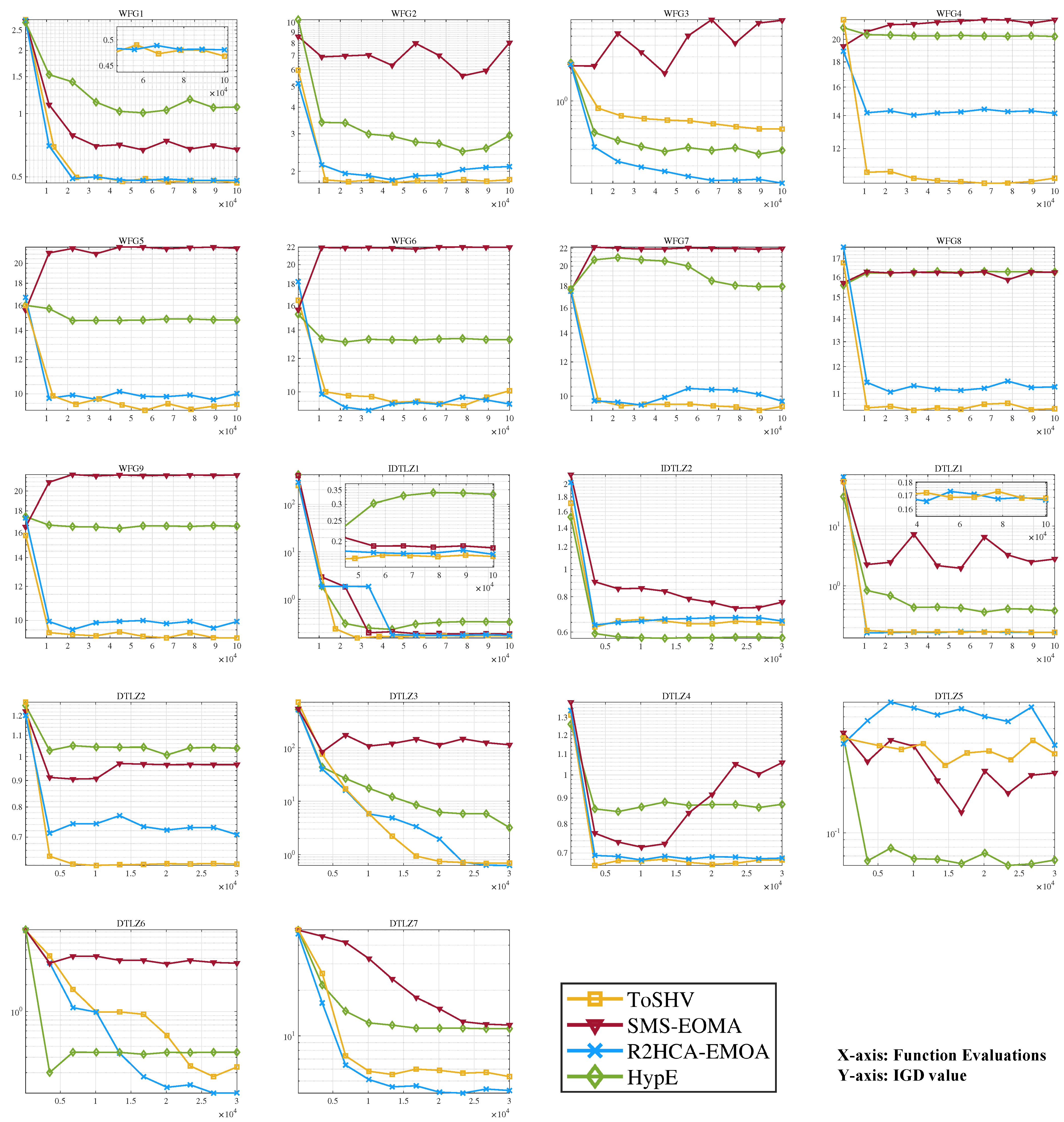

Figure A2.
IGD variations over function evaluations obtained with AR−MOEA, DGEA, MOEA/DD, NSGA−III, and ToSHV on WFG 1−9, IDTLZ 1−2, and DTLZ 1−7 problems with 15 objectives.
Figure A2.
IGD variations over function evaluations obtained with AR−MOEA, DGEA, MOEA/DD, NSGA−III, and ToSHV on WFG 1−9, IDTLZ 1−2, and DTLZ 1−7 problems with 15 objectives.
Appendix C. The Distribution of the Solutions Obtained by the Algorithms in Different Problems

Figure A3.
The solution distribution of ToSHV and three hypervolume-based EMOAs on 15-dimensional WFG5, WFG6, DTLZ1, DTLZ3, IDTLZ1, and IDTLZ2 problems.
Figure A3.
The solution distribution of ToSHV and three hypervolume-based EMOAs on 15-dimensional WFG5, WFG6, DTLZ1, DTLZ3, IDTLZ1, and IDTLZ2 problems.

Figure A4.
Distribution of solutions obtained by AR-MOEA, DGEA, MOEA/DD, NSGA-III, and ToSHV on the 3-objective problems.
Figure A4.
Distribution of solutions obtained by AR-MOEA, DGEA, MOEA/DD, NSGA-III, and ToSHV on the 3-objective problems.
References
- Farina, M.; Amato, P. On the optimal solution definition for many-criteria optimization problems. In Proceedings of the 2002 Annual Meeting of the North American Fuzzy Information Processing Society Proceedings, NAFIPS-FLINT 2002 (Cat. No. 02TH8622), New Orleans, LA, USA, 27–29 June 2002; pp. 233–238. [Google Scholar]
- Deb, K.; Pratap, A.; Agarwal, S.; Meyarivan, T. A fast and elitist multiobjective genetic algorithm: NSGA-II. IEEE Trans. Evol. Comput. 2002, 6, 182–197. [Google Scholar] [CrossRef]
- Zitzler, E.; Laumanns, M.; Thiele, L. SPEA2: Improving the strength Pareto evolutionary algorithm. TIK Rep. 2001, 103. [Google Scholar] [CrossRef]
- Ou, J.; Zheng, J.; Ruan, G.; Hu, Y.; Zou, J.; Li, M.; Yang, S.; Tan, X. A pareto-based evolutionary algorithm using decomposition and truncation for dynamic multi-objective optimization. Appl. Soft Comput. 2019, 85, 105673. [Google Scholar] [CrossRef]
- Zou, J.; Liu, J.; Yang, S.; Zheng, J. A many-objective evolutionary algorithm based on rotation and decomposition. Swarm Evol. Comput. 2021, 60, 100775. [Google Scholar] [CrossRef]
- Elarbi, M.; Bechikh, S.; Gupta, A.; Said, L.B.; Ong, Y.S. A New Decomposition-Based NSGA-II for Many-Objective Optimization. IEEE Trans. Syst. Man Cybern. Syst. 2018, 48, 1191–1210. [Google Scholar] [CrossRef]
- Laumanns, M.; Thiele, L.; Deb, K.; Zitzler, E. Combining convergence and diversity in evolutionary multiobjective optimization. Evol. Comput. 2002, 10, 263–282. [Google Scholar] [CrossRef]
- Zhang, Q.; Li, H. MOEA/D: A multiobjective evolutionary algorithm based on decomposition. IEEE Trans. Evol. Comput. 2007, 11, 712–731. [Google Scholar] [CrossRef]
- Deb, K.; Jain, H. An evolutionary many-objective optimization algorithm using reference-point-based nondominated sorting approach, part I: Solving problems with box constraints. IEEE Trans. Evol. Comput. 2013, 18, 577–601. [Google Scholar] [CrossRef]
- Li, K.; Deb, K.; Zhang, Q.; Kwong, S. An evolutionary many-objective optimization algorithm based on dominance and decomposition. IEEE Trans. Evol. Comput. 2014, 19, 694–716. [Google Scholar] [CrossRef]
- Yang, X.; Wu, L.; Zhang, H. A space-time spectral order sinc-collocation method for the fourth-order nonlocal heat model arising in viscoelasticity. Appl. Math. Comput. 2023, 457, 128192. [Google Scholar] [CrossRef]
- Jiang, X.; Wang, J.; Wang, W.; Zhang, H. A Predictor-Corrector Compact Difference Scheme for a Nonlinear Fractional Differential Equation. Fractal Fract. 2023, 7, 521. [Google Scholar] [CrossRef]
- Ishibuchi, H.; Setoguchi, Y.; Masuda, H.; Nojima, Y. Performance of decomposition-based many-objective algorithms strongly depends on Pareto front shapes. IEEE Trans. Evol. Comput. 2016, 21, 169–190. [Google Scholar] [CrossRef]
- Qi, Y.; Ma, X.; Liu, F.; Jiao, L.; Sun, J.; Wu, J. MOEA/D with adaptive weight adjustment. Evol. Comput. 2014, 22, 231–264. [Google Scholar] [CrossRef] [PubMed]
- Cheng, R.; Jin, Y.; Olhofer, M.; Sendhoff, B. A reference vector guided evolutionary algorithm for many-objective optimization. IEEE Trans. Evol. Comput. 2016, 20, 773–791. [Google Scholar] [CrossRef]
- Asafuddoula, M.; Singh, H.K.; Ray, T. An enhanced decomposition-based evolutionary algorithm with adaptive reference vectors. IEEE Trans. Cybern. 2017, 48, 2321–2334. [Google Scholar] [PubMed]
- Zhu, F.; Zhong, P.A.; Sun, Y.; Xu, B.; Ma, Y.; Liu, W.; Zhang, D.; Dawa, J. A coordinated optimization framework for long-term complementary operation of a large-scale hydro-photovoltaic hybrid system: Nonlinear modeling, multi-objective optimization and robust decision-making. Energy Convers. Manag. 2020, 226, 113543. [Google Scholar] [CrossRef]
- Zhao, L.; Wang, B.; Jiang, X.; Lu, Y.; Hu, Y. DIP-MOEA: A double-grid interactive preference based multi-objective evolutionary algorithm for formalizing preferences of decision makers. Front. Inf. Technol. Electron. Eng. 2022, 23, 1714–1732. [Google Scholar] [CrossRef]
- Pang, Y.; Wang, Y.; Zhang, S.; Lai, X.; Sun, W.; Song, X. An Expensive Many-Objective Optimization Algorithm Based on Efficient Expected Hypervolume Improvement. IEEE Trans. Evol. Comput. 2022. [Google Scholar] [CrossRef]
- Zitzler, E.; Thiele, L. Multiobjective optimization using evolutionary algorithms—A comparative case study. In Proceedings of the International Conference on Parallel Problem Solving from Nature, Amsterdam, The Netherlands, 27–30 September 1998; Springer: Berlin/Heidelberg, Germany, 1998; pp. 292–301. [Google Scholar]
- Coello Coello, C.A.; Reyes Sierra, M. A study of the parallelization of a coevolutionary multi-objective evolutionary algorithm. In Proceedings of the MICAI 2004: Advances in Artificial Intelligence: Third Mexican International Conference on Artificial Intelligence, Mexico City, Mexico, 26–30 April 2004; Springer: Berlin/Heidelberg, Germany, 2004; pp. 688–697. [Google Scholar]
- Hansen, M.P.; Jaszkiewicz, A. Evaluating the Quality of Approximations to the Non-Dominated Set; IMM, Department of Mathematical Modelling, Technical Universityof Denmark: Copenhagen, Denmark, 1994. [Google Scholar]
- Guerreiro, A.P.; Fonseca, C.M.; Paquete, L. The hypervolume indicator: Computational problems and algorithms. ACM Comput. Surv. (CSUR) 2021, 54, 1–42. [Google Scholar] [CrossRef]
- Beume, N.; Naujoks, B.; Emmerich, M. SMS-EMOA: Multiobjective selection based on dominated hypervolume. Eur. J. Oper. Res. 2007, 181, 1653–1669. [Google Scholar] [CrossRef]
- Jiang, S.; Zhang, J.; Ong, Y.S.; Zhang, A.N.; Tan, P.S. A simple and fast hypervolume indicator-based multiobjective evolutionary algorithm. IEEE Trans. Cybern. 2014, 45, 2202–2213. [Google Scholar] [CrossRef] [PubMed]
- Bader, J.; Zitzler, E. HypE: An algorithm for fast hypervolume-based many-objective optimization. Evol. Comput. 2011, 19, 45–76. [Google Scholar] [CrossRef] [PubMed]
- Shang, K.; Ishibuchi, H. A new hypervolume-based evolutionary algorithm for many-objective optimization. IEEE Trans. Evol. Comput. 2020, 24, 839–852. [Google Scholar] [CrossRef]
- Shang, K.; Ishibuchi, H.; Ni, X. R2-based hypervolume contribution approximation. IEEE Trans. Evol. Comput. 2019, 24, 185–192. [Google Scholar] [CrossRef]
- Wen, C.; Li, L.; Peng, Z. A Hypervolume-based evolutionary algorithm for Many-objective optimization. In Proceedings of the International Workshop on Advanced Computational Intelligence and Intelligent Informatics, Jahangirnagar, Bangladesh, 14–15 October 2023. [Google Scholar]
- Huband, S.; Hingston, P.; Barone, L.; While, L. A review of multiobjective test problems and a scalable test problem toolkit. IEEE Trans. Evol. Comput. 2006, 10, 477–506. [Google Scholar] [CrossRef]
- Tian, Y.; Cheng, R.; Zhang, X.; Jin, Y. PlatEMO: A MATLAB platform for evolutionary multi-objective optimization [Educational forum]. IEEE Comput. Intell. Mag. 2017, 12, 73–87. [Google Scholar] [CrossRef]
- He, C.; Cheng, R.; Yazdani, D. Adaptive offspring generation for evolutionary large-scale multiobjective optimization. IEEE Trans. Syst. Man Cybern. Syst. 2020, 52, 786–798. [Google Scholar] [CrossRef]
- Tian, Y.; Cheng, R.; Zhang, X.; Cheng, F.; Jin, Y. An indicator-based multiobjective evolutionary algorithm with reference point adaptation for better versatility. IEEE Trans. Evol. Comput. 2017, 22, 609–622. [Google Scholar] [CrossRef]
- Zhang, H.; Liu, Y.; Yang, X. An efficient ADI difference scheme for the nonlocal evolution problem in three-dimensional space. J. Appl. Math. Comput. 2023, 69, 651–674. [Google Scholar] [CrossRef]
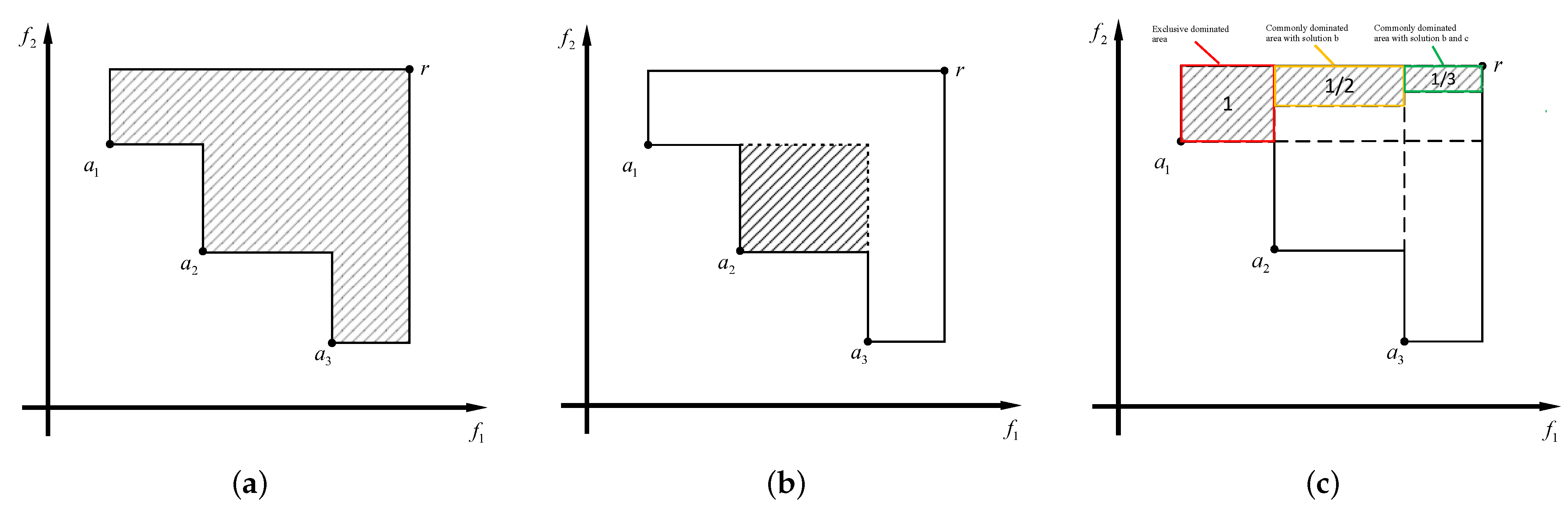
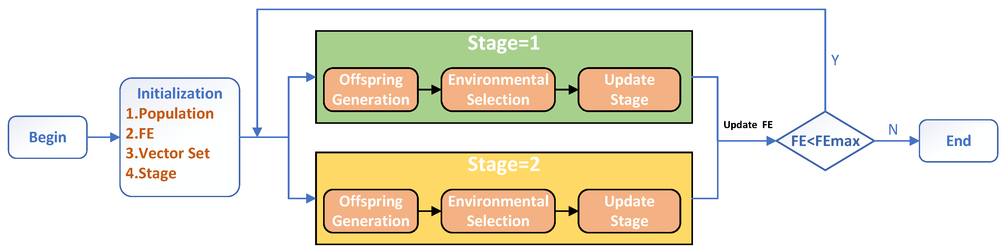
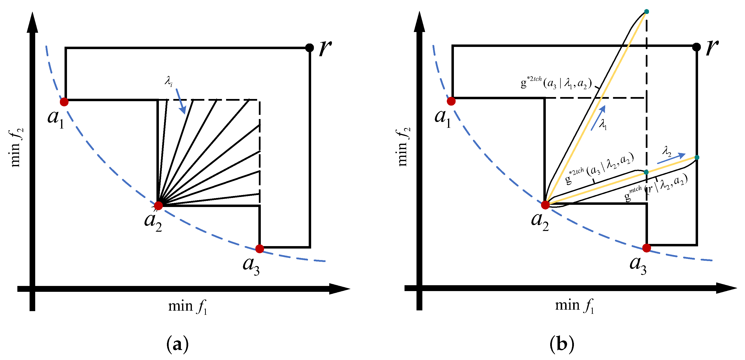
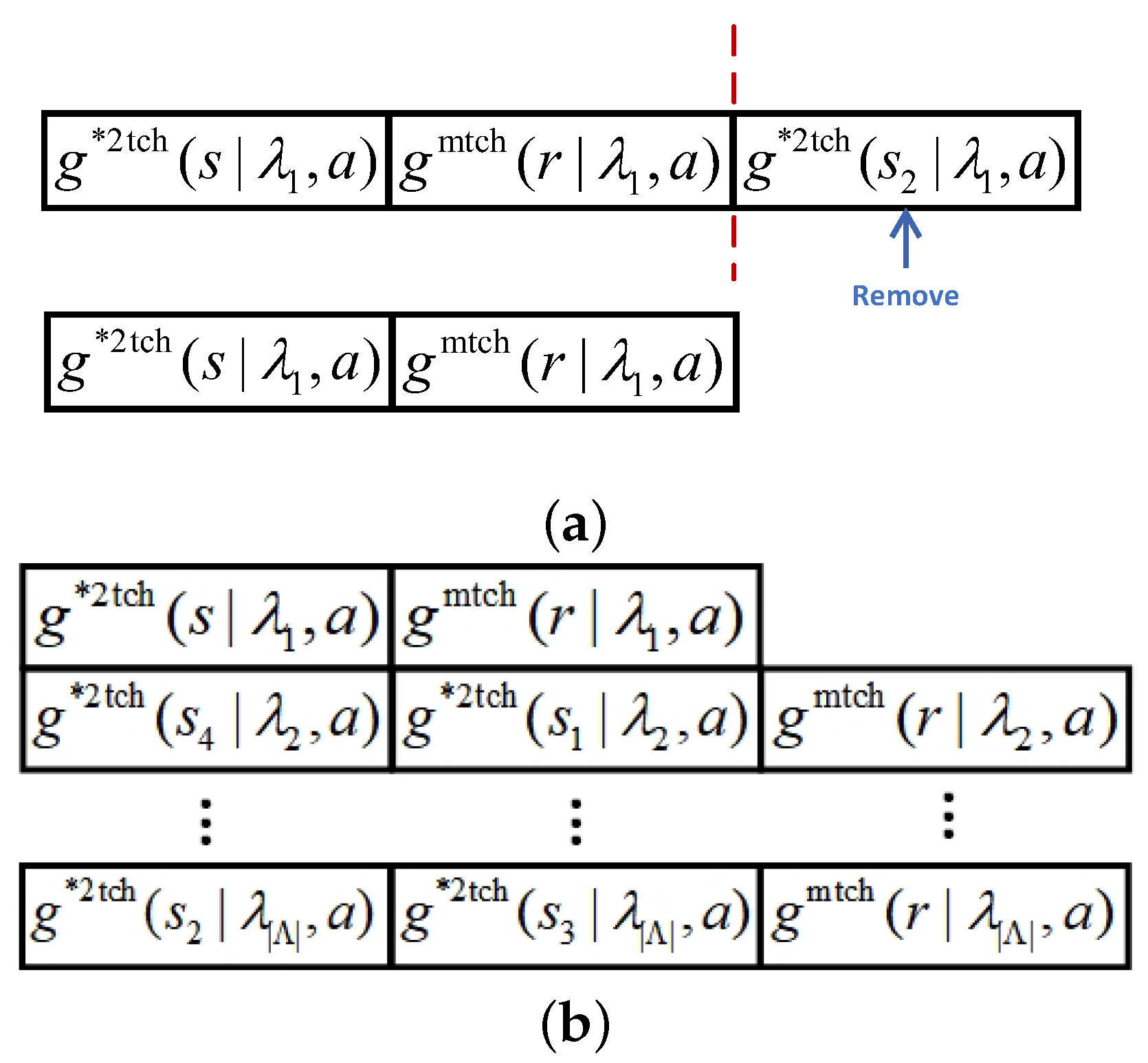
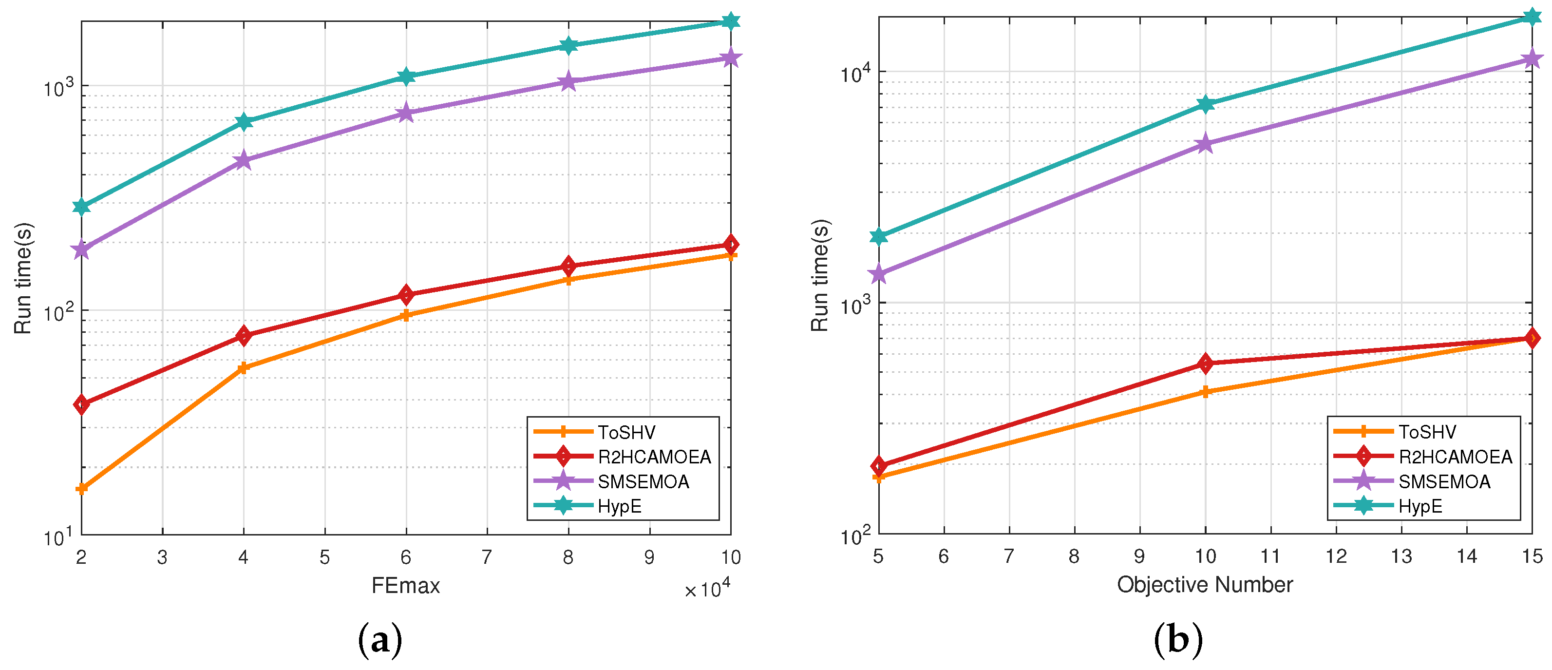
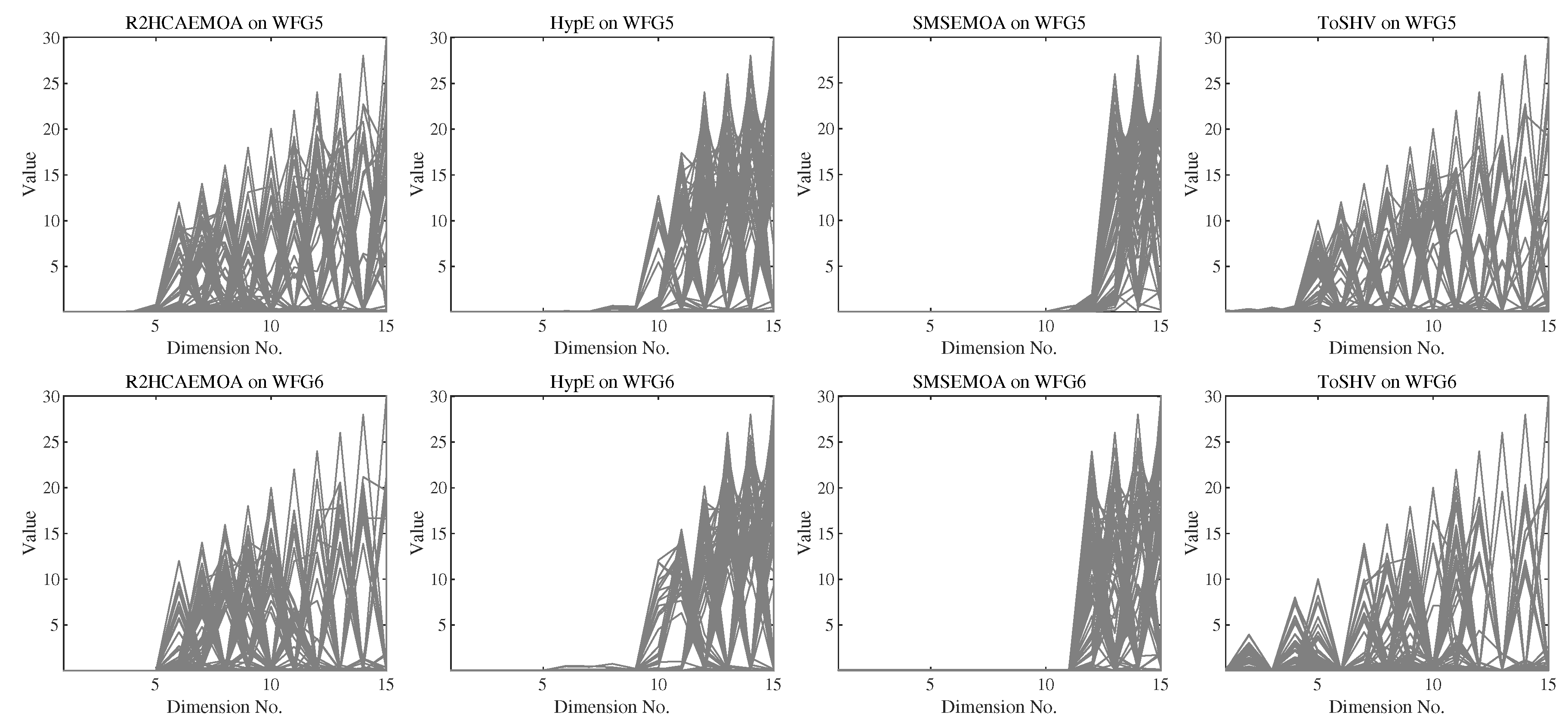
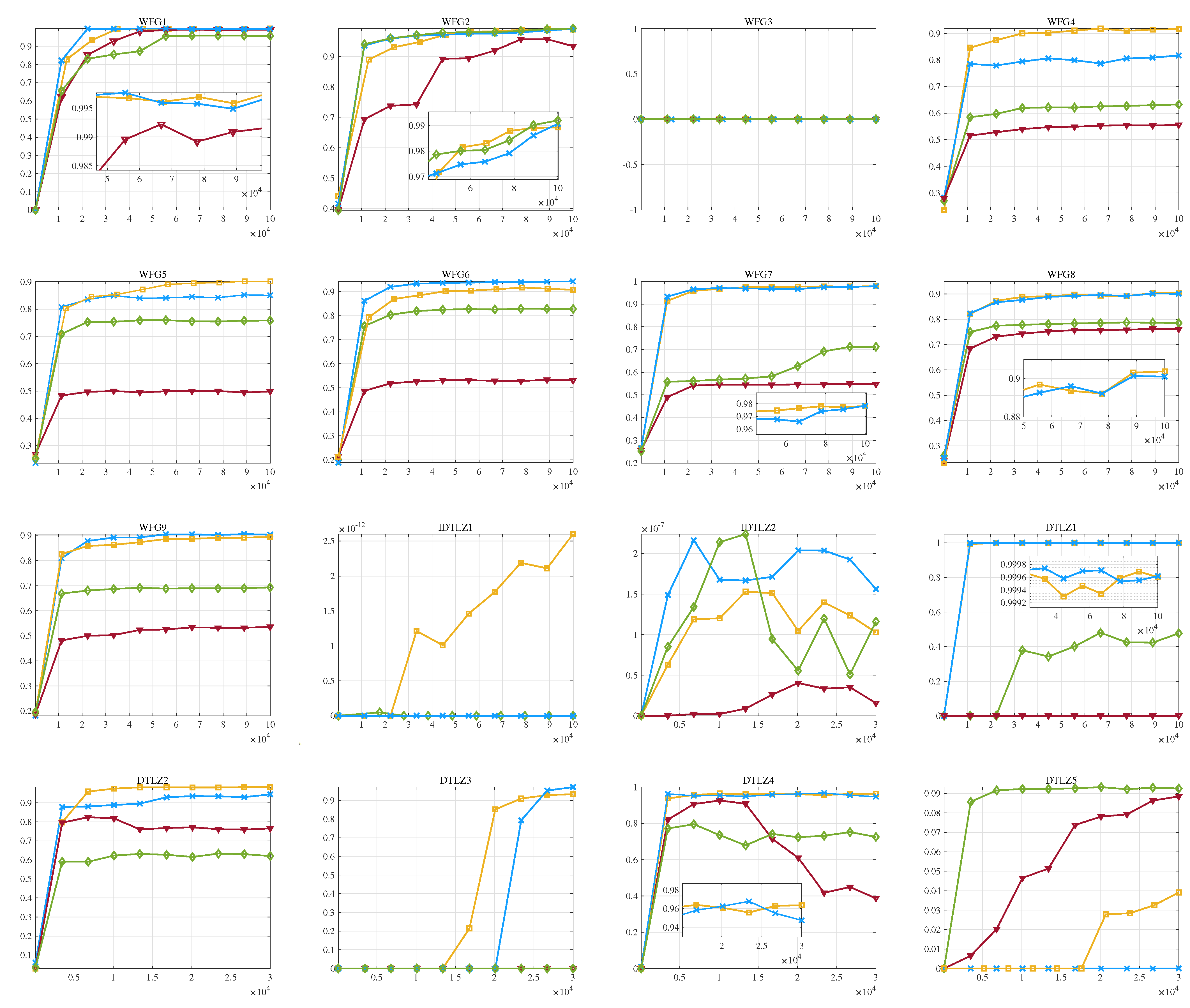
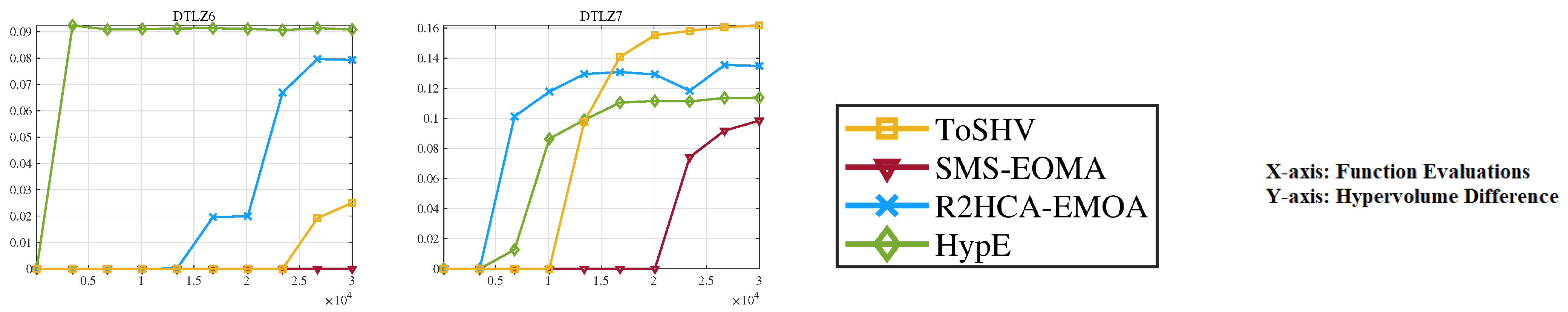
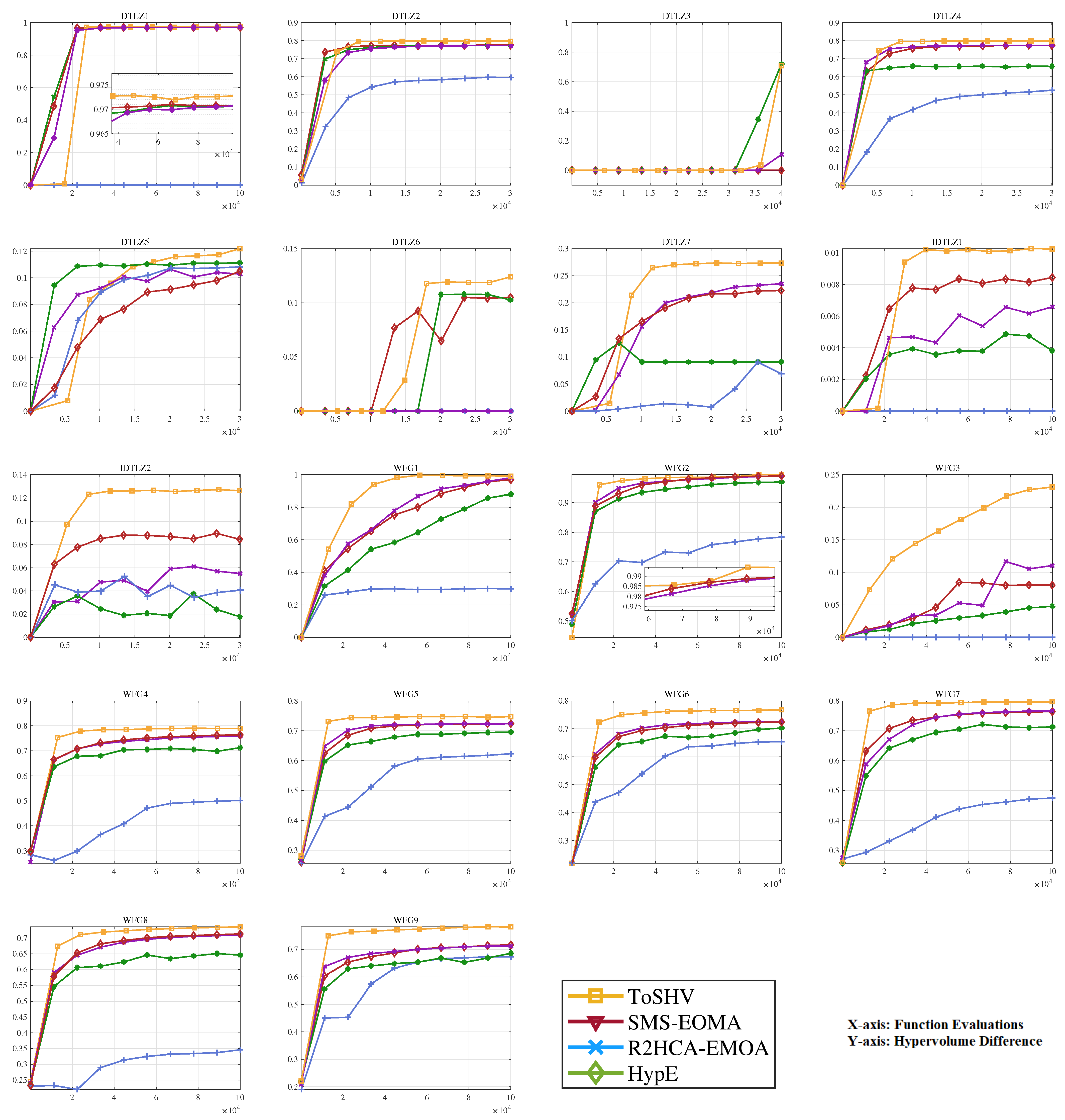
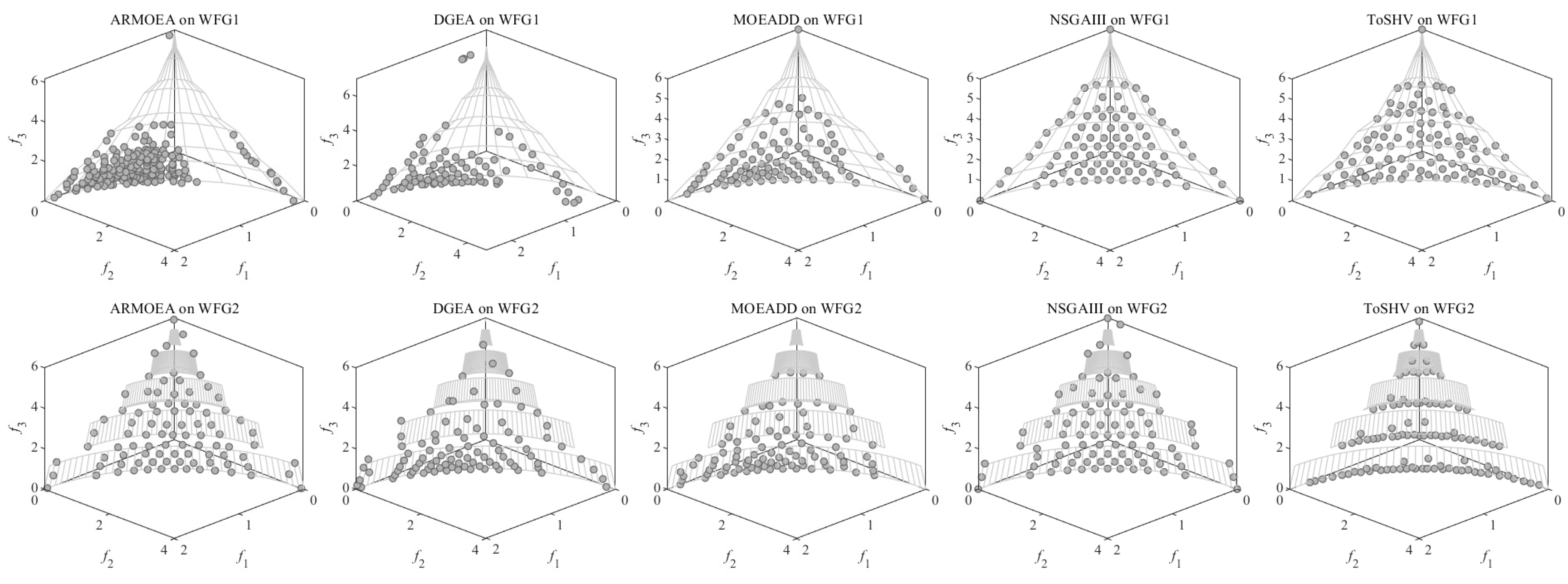
Disclaimer/Publisher’s Note: The statements, opinions and data contained in all publications are solely those of the individual author(s) and contributor(s) and not of MDPI and/or the editor(s). MDPI and/or the editor(s) disclaim responsibility for any injury to people or property resulting from any ideas, methods, instructions or products referred to in the content. |
© 2023 by the authors. Licensee MDPI, Basel, Switzerland. This article is an open access article distributed under the terms and conditions of the Creative Commons Attribution (CC BY) license (https://creativecommons.org/licenses/by/4.0/).