Abstract
The zeros of the reliability polynomials of circular consecutive-k-out-of-n:F systems are studied. We prove that, for any fixed , the set of the roots of all the reliability polynomials (for all ) is unbounded in the complex plane. In the particular case , we show that all the nonzero roots are real, distinct numbers and find the closure of the set of roots. For every , the expressions of the minimum root and the maximum root are given, both for circular as well as for linear systems.
Keywords:
consecutive-k-out-of-n:F systems; reliability polynomial; Beraha–Kahane–Weiss theorem; Fibonacci polynomials; Jacobsthal polynomials; Lucas polynomials MSC:
11B39; 11B37; 05C31; 26C10; 30C15
1. Introduction
Consecutive-k-out-of-n:F systems were introduced by Kontoleon [1] under the name of “r-successive-out-of-n:F”, being re-branded “consecutive-k-out-of-n:F” one year later [2]. They have attracted researchers’ interest due to their robustness and ability to achieve high reliability at reasonably low costs. A consecutive-k-out-of-n:F system is formed by n components placed in a row (if the system is linear), or in a cycle (for a circular system, a concept mentioned for the first time in [3]), which fails if and only if at least k consecutive components fail. The reader can find a detailed presentation of the subject in [4,5,6] and recent contributions in the field, developments, and applications in [7,8,9,10,11,12,13,14,15,16,17,18].
A linear consecutive-k-out-of-n:F system can be represented as a graph , with vertices, , and having the set of edges (see Figure 1). The nodes are identical and statistically independent, failing with probability , while the terminals , , as well as the edges, are always operational. Note that this graph representation may be directed or undirected. The reliability of the system, denoted by , is the probability that the system is working, i.e., the probability that the subgraph induced by the operational nodes has at least one path linking the terminal nodes S and T.
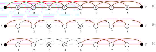
Figure 1.
Linear consecutive-2-out-of-8:F system: (a) the nodes are operational with probability p; (b) two non-consecutive nodes (3 and 5) have failed, the system works; (c) two consecutive nodes (3 and 4) have failed, the system fails.
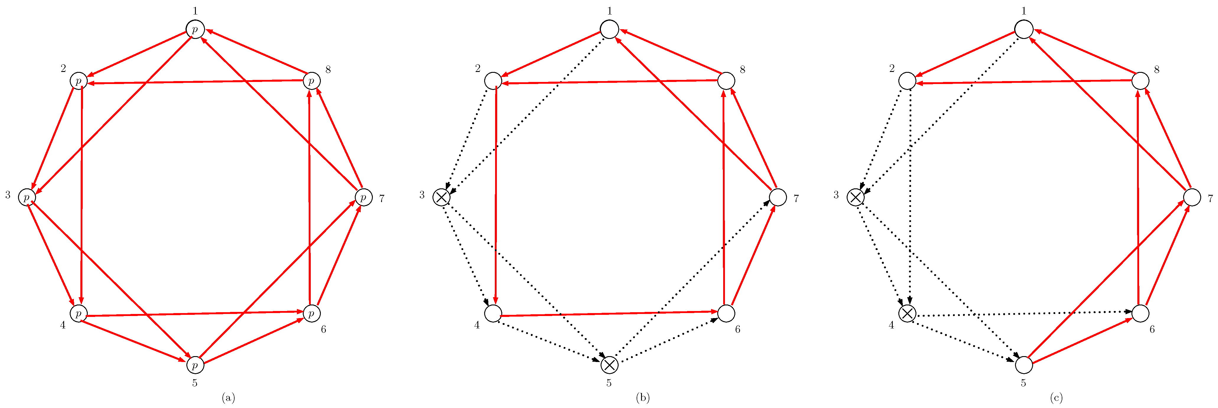
A circular consecutive-k-out-of-n:F system can also be represented as a directed graph , with n vertices, , and having the set of directed edges (see Figure 2). As in the linear case, we assume that the nodes are identical and statistically independent, failing with probability , while the edges are always operational. The reliability of the circular system, , is the probability that the subgraph induced by the operational nodes is Hamiltonian (it has a cycle that visits each vertex exactly once).
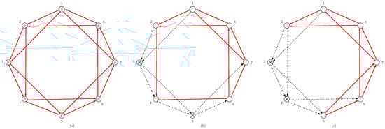
Figure 2.
Circular consecutive-2-out-of-8:F system: (a) the nodes are operational with probability p; (b) two non-consecutive nodes (3 and 5) have failed, the system works; (c) two consecutive nodes (3 and 4) have failed, the system fails.
In both cases, the reliability is a polynomial of degree n in p, for every (for , it is equal to 1). Moreover, these reliability polynomials satisfy the same recurrence relation, for every in the linear case, and for every in the circular case, respectively. Philippou [19] identified the relation between the reliability polynomials of linear consecutive systems and the generalized Fibonacci polynomials (introduced by Hoggatt and Bicknell in [20]), while Charalambides [21] noted the relation between the reliability polynomials of circular consecutive systems and the Lucas polynomials of order k.
The reliability polynomial of a network formed by a number of identical components is usually considered as a function of p, the probability that a single component is functional. The value of p is normally supposed to be in the interval , but studying the analytic properties of these polynomials as functions of a complex variable can shed new light on the landscape of reliability theory. Originally [22], the roots of reliability polynomials were investigated for the possible log-concavity of the coefficients. In fact, various properties of the roots can be linked to the shape of the coefficients [23], so finding the location and magnitude of the roots is clearly worth exploring.
For instance, using the Newton’s inequalities (see [24], 7.1), it can be easily shown that for any polynomial with positive coefficients and real roots, the sequence of coefficients is log-concave, that is,
It is well-known that a log-concave sequence is unimodal. As a matter of fact, the condition above is sufficient, but it is not necessary. A more general result [25] states that if all the (complex) roots of a polynomial with positive coefficients lie in the region , then the sequence of coefficients is log-concave.
Finding the set of roots of various polynomials related to different families of graphs is both a tempting and also a fruitful problem which has attracted lots of research in the past few decades (see, for instance [22,26,27,28,29,30] for reliability polynomials; [31,32,33,34,35] for chromatic polynomials; and [36,37,38,39] for independence polynomials). In many of these papers, a central role is played by a theorem on analytic functions due to Beraha, Kahane, and Weiss [40], which proves to be a highly useful instrument to study the zeros of a family of polynomials defined recursively.
Using the Beraha–Kahane–Weiss theorem, the authors have proven in a recent paper [41] that the set of the roots of the reliability polynomials of linear consecutive-k-out-of-n:F systems is unbounded, for any . In this paper, we show (in Section 2) that the result also holds for circular consecutive-k-out-of-n:F systems. In Section 3, we study the particular case when and prove that all the nonzero roots of the reliability polynomial of the circular consecutive-2-out-of-n:F system are real, distinct numbers (for any ). Moreover, we show that any root of a circular consecutive-2-out-of-n:F system is also a root of the linear consecutive-2-out-of-:F system. Finally, in Section 4 we investigate the values of the minimum and the maximum root for different values of n, and for both kinds of systems. We show that the interval between the minimum and the maximum root is growing faster (as n increases) for circular systems than for linear systems. It is also worth mentioning that, in each case, the sequence of intervals exhibits a kind of periodicity, being formed by three monotonic subsequences.
2. The Circular Consecutive--out-of-:F Systems Have Unbounded Roots
For any fixed , the reliability polynomials of circular consecutive-k-out-of-n:F systems satisfy the following recurrence relation for any (see [42]):
Since the system fails if and only if at least k consecutive components fail, the first k polynomials are equal to 1:
and when :
For , the reliability polynomials have the expression [42]:
Since is fixed, for any , the polynomial can be written as follows:
where
and is a polynomial of degree n in z. From (1), we find that the polynomials satisfy the following recurrence relation, for any :
In the following, we recall some basic results on recursively defined polynomials. Consider an arbitrary sequence of polynomials , , defined by a linear recurrence relation of order k:
where and , are given polynomials.
We say that is a limit of zeros of if there exists a sequence of complex numbers such that and .
Let , be the roots of the characteristic equation
Then, for any such that for , one can write:
where , are found from the linear system of equations obtained by writing (11) for .
Theorem 1
(Beraha–Kahane–Weiss theorem [40]). Suppose that is a sequence of polynomials defined by a relation of the form (9) such that satisfies no recursion of order less than k, and there is no constant ω, with , such that for some .
Then, x is a limit of zeros of if and only if the roots of the characteristic Equation (10) can be ordered such that one of the following holds:
(i) for every , and ,
(ii) , , for some .
Using this theorem, we can prove the following result.
Theorem 2.
For any fixed , the set of complex roots of all the polynomials , , is unbounded.
Proof.
First, we prove that the sequence of polynomials defined by the recurrence (7) of order k, with the initial conditions (8), satisfies the conditions from Theorem 1. In our case, the characteristic Equation (10) is written
Suppose that there exists a constant with with the property that for any , there exists a root of (12) such that is also a root of (12).
We can bring Equation (12) to a simpler form if we multiply it by . Thus, we can see that any root of (12) also satisfies the equation
while (13) has a root (namely, ) which is not a root of (12).
For , the characteristic Equation (12) becomes
and its roots are the roots of the Equation (13), which is written:
If k is odd, the complex roots of this equation are
while for k even, the roots are of the form:
In any case, the roots of the characteristic Equation (14) are all distinct complex numbers of modulus 1:
and we can see that the ratio between any two different roots is of the form
Thus, if there were a constant such that, for any z, there exist two roots and of (12), then should be of the form (16), and hence it should satisfy .
Consider . Then, the roots of (13) are different from 0. If we suppose that both and satisfy Equation (13), then we obtain that , a contradiction, which implies that there is no such constant . So we find (using (15)) that the hypotheses of Theorem 1 case (ii) are fulfilled, and hence there exists a sequence of complex numbers such that and .
3. The Roots of Consecutive-2-out-of-:F Systems
In this section, we study the particular case of circular consecutive-2-out-of-n systems and find the explicit formula for the reliability polynomials and their roots (proved to be all real numbers). We also aim to compare the circular and the linear consecutive-2-out-of-n systems, underlying the similarities and differences, as well as the relationships between the two families of polynomials. Therefore, we begin with a short review of the reliability polynomials of linear consecutive systems (studied in [41]).
The reliability polynomials of linear consecutive-k-out-of n:F systems satisfy the same recurrence relation as [4], but starting from (while the polynomials of circular systems satisfy the recurrence relation (1) starting from ):
for every . The initial polynomials are
Using the same transformation, , and , we obtain the sequence of polynomials satisfying the same recurrence as
for every and the initial conditions
Thus, as noted in [41], the sequence is the sequence of Jacobsthal polynomials , with . Introduced in [43], the Jacobsthal polynomials have the same coefficients as the more famous Fibonacci polynomials, being related by the formula (see ([44], Chp. 44) for a detailed presentation). Table 1 shows the Fibonacci polynomials and Jacobsthal polynomials for .

Table 1.
Fibonacci and Jacobsthal polynomials.
The Jacobsthal polynomials can be expressed by the following Binet-type formula [44]:
hence,
for every .
The Jacobsthal polynomials are closely related to the Jacobsthal–Lucas polynomials defined by the same recurrence relation,
but with the initial terms , [44,45]. These polynomials have the same coefficients as the well-known Lucas polynomials (defined by the same recurrence relation as the Fibonacci polynomials, but with different initial terms), being related by the formula (see Table 2).
Table 2.
Lucas and Jacobsthal–Lucas polynomials.
Now, if we consider the polynomials corresponding to the circular consecutive-2-out-of-n:F systems, , we can see that for , the relations (7) and (8) become:
and we notice that , for every .
Obviously, the characteristic equation corresponding to the recurrence relation (28) is again (24), having the roots and expressed by (25), so the polynomial can be written:
Using the initial conditions (29), it can be easily shown , so we obtain the following Binet-type formula (the same as the expression of Jacobsthal–Lucas polynomials [44]):
for every .
Remark 1.
Moreover, the following identity can be proved using (32) and mathematical induction on :
The roots of the of linear consecutive-2-out-of-n:F systems were studied in [41], and it has been proved that for any , the nonzero roots of the reliability polynomial are real, distinct numbers. The Formula (32) allows us to state the same for circular consecutive-2-out-of-n:F systems. In particular, the next theorem establishes a stronger statement, namely that the closure of the set of roots of the reliability polynomials of circular consecutive-2-out-of-n:F systems is the same as for the linear consecutive case.
Theorem 3.
For any , the nonzero roots of the reliability polynomial of the circular consecutive-2-out-of-n:F system are real, distinct numbers.
Let and denote the set of roots (for all ) of the polynomials and , respectively. Then,
and
Proof.
According to (32), it follows that all the roots of the polynomial are also roots of the polynomial . Hence, , and from ([41], Theorem 3), it readily follows that the nonzero roots of are distinct, real numbers.
In order to prove (35), we need the explicit expression of these roots. From (5), we have that every nonzero root of corresponds to a root of the polynomial . Using (30), we have:
It follows that
are the distinct roots of the polynomial . It can be easily seen that for any r; hence,
are the distinct nonzero roots of the reliability polynomial . Using (37), it can be seen that for every and , and the roots are dense in . □
4. Discussion
Finally, we compare the roots of circular consecutive-2-out-of-n:F systems (37) against the ones of linear consecutive-2-out-of-n:F systems (obtained in [41]):
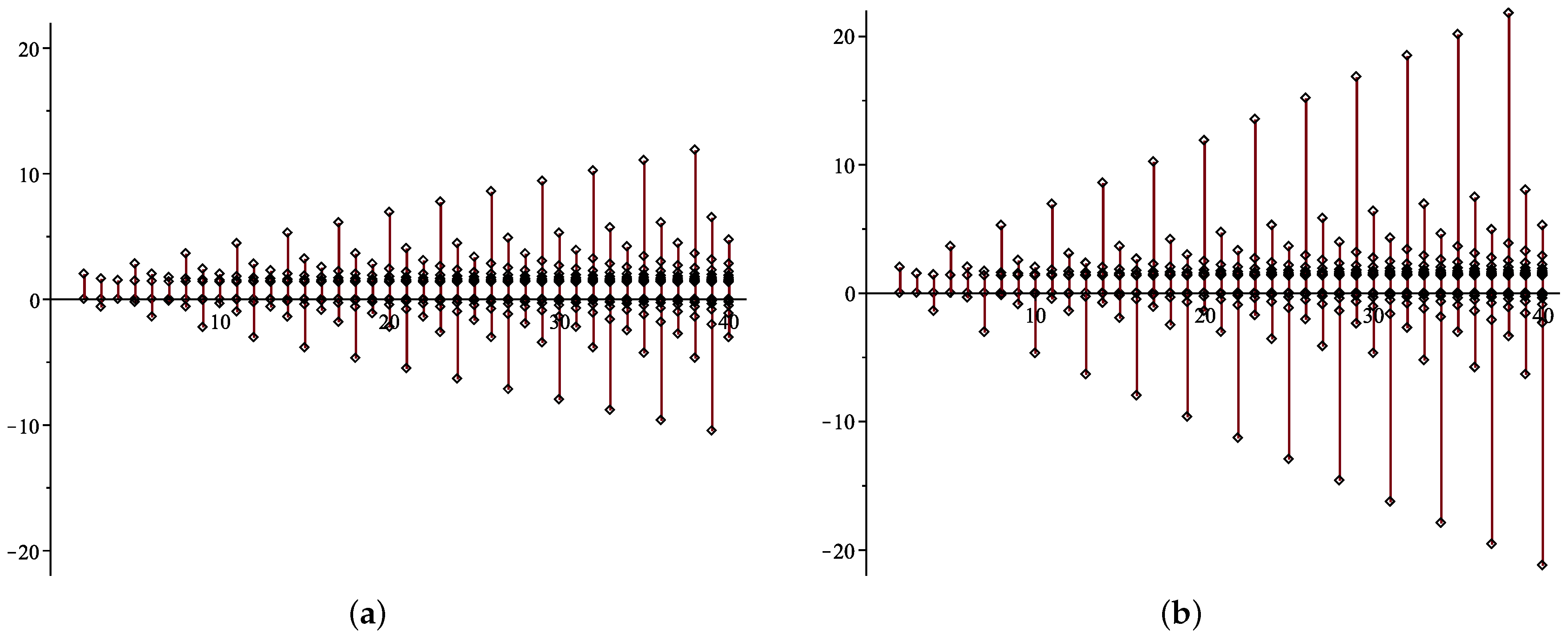
We present in Figure 3 the roots of the reliability polynomials of consecutive-2-out-of-n systems, when for both cases: linear systems (a) and circular systems (b).
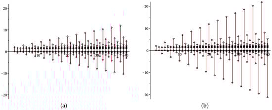
Figure 3.
(a) The roots of the linear consecutive 2-out-of-n systems; (b) the roots of the circular consecutive 2-out-of-n systems; .
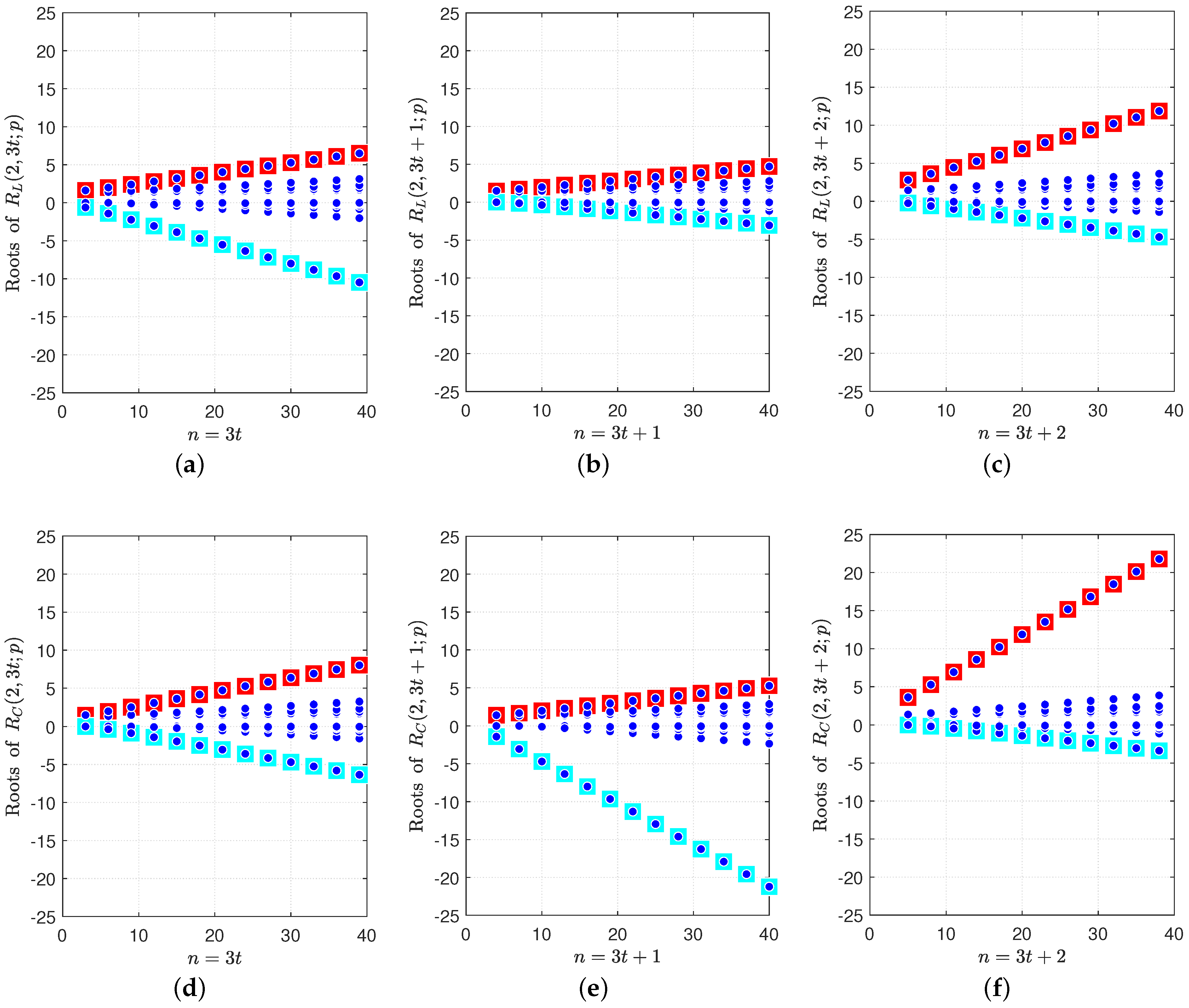
It can be noticed that, as n increases, the interval between the minimum and the maximum root is growing faster for circular systems than for linear systems. Another remark is that the sequence of intervals can be split into three monotone subsequences: for , , and (see Figure 4).

Figure 4.
The roots for n in the range as blue circles (maxima as red squares, and minima as cyan squares) for linear consecutive-2-out-of-n:F systems: (a) , (b) , (c) ; for circular consecutive-2-out-of-n:F systems: (d) , (e) ; (f) .
Let us calculate the maximum and the minimum value of and , for every . The extreme values in (38) are attained when the denominator of the fraction is as close at possible (but not equal) to 0. Hence, for every , the maximum value is obtained for , while the minimum value occurs for :
Using the same reasoning for circular consecutive-2-out-of-n:F systems (with the remark that in (37) the denominator never vanishes), we find that the maximum root is obtained for , while the minimum one occurs for , for any :
5. Conclusions
This paper has investigated the roots of the reliability polynomials of circular consecutive-k-out-of-n:F systems, showing the similarities and the differences between circular and linear consecutive systems (studied in [41]). Using the Beraha–Kahane–Weiss theorem, we have proved that the roots of circular consecutive-k-out-of-n:F systems are unbounded, for any .
In the particular case when , the reliability polynomials of linear and of circular consecutive-2-out-of-n:F systems are shown to be related to the Jacobsthal and Jacobsthal–Lucas polynomials, respectively. Thus, the relation between the two families of polynomials is revealed to be the same as the relation between Fibonacci and Lucas polynomials: both sequences of polynomials have the same recurrence relation, but different initial values.
Using the explicit expression deduced from the recurrence formula, we have shown that the roots of of circular consecutive-2-out-of-n:F systems share the same properties as the roots of linear consecutive-2-out-of-n:F systems, namely, that for every , all the nonzero roots are distinct, real numbers contained into the union of intervals .
Moreover, the set of all the roots of circular consecutive-2-out-of-n:F systems is a subset of the set of roots of the linear consecutive systems, and both sets are dense in the union of intervals above. However, the roots of circular systems exhibit a faster spreading along the real axis than the roots of linear consecutive-2-out-of-n:F systems.
Author Contributions
Conceptualization, M.J. and L.D.; methodology, L.D. and V.B.; software, V.-F.D. and V.B.; validation, V.-F.D. and V.B.; writing—original draft preparation, M.J.; writing—review and editing, M.J., L.D., V.-F.D. and V.B.; project administration, V.B.; funding acquisition, V.B. All authors have read and agreed to the published version of the manuscript.
Funding
This research was partly funded by a grant of the Romanian Ministry of Education and Research, CNCS-UEFISCDI, project no. PN-III-P4-ID-PCE-2020-2495, within PNCDI III (ThUNDER2 = Techniques for Unconventional Nano-Designing in the Energy-Reliability Realm).
Institutional Review Board Statement
Not applicable.
Informed Consent Statement
Not applicable.
Data Availability Statement
Not applicable.
Conflicts of Interest
The authors declare no conflict of interest.
References
- Kontoleon, J.M. Reliability determination of a r-succesive-out-of-n:F system. IEEE Trans. Reliab. 1980, R-29, 437. [Google Scholar] [CrossRef]
- Chiang, D.T.; Niu, S. Reliability of consecutive-k-out-of-n:F system. IEEE Trans. Reliab. 1981, R-30, 87–89. [Google Scholar] [CrossRef]
- Derman, C.; Lieberman, G.J.; Ross, S.M. On the consecutive-k-out-of-n:F system. IEEE Trans. Reliab. 1982, R-31, 57–63. [Google Scholar] [CrossRef]
- Chang, G.J.; Cui, L.; Hwang, F.K. Reliabilities of Consecutive-k Systems; Springer: New York, NY, USA, 2000. [Google Scholar]
- Kuo, W.; Zuo, M.J. Optimal Reliability Modeling: Principles and Applications; John Wiley & Sons: Hoboken, NJ, USA, 2003. [Google Scholar]
- Chao, M.T.; Fu, J.C.; Koutras, M.V. Survey of reliability studies of consecutive-k-out-of-n:F & related systems. IEEE Trans. Reliab. 1995, 44, 120–127. [Google Scholar]
- Triantafyllou, I.S.; Koutras, M.K. Reliability properties of (n,f,k) systems. IEEE Trans. Reliab. 2014, 63, 357–366. [Google Scholar] [CrossRef]
- Beiu, V.; Dăuş, L. Reliability bounds for two dimensional consecutive systems. Nano Comm. Netw. 2015, 6, 145–152. [Google Scholar] [CrossRef]
- Dăuş, L.; Beiu, V. Lower and upper reliability bounds for consecutive-k-out-of-n:F systems. IEEE Trans. Reliab. 2015, 64, 1128–1135. [Google Scholar] [CrossRef]
- Mohammadi, F.; Sáenz-de-Cabezón, E.; Wynn, H.P. Efficient multicut enumeration of k-out-of-n:F and consecutive k-out-of-n:F systems. Pattern Recog. Lett. 2018, 102, 82–88. [Google Scholar] [CrossRef]
- Dafnis, S.D.; Makri, F.S.; Philippou, A.N. The reliability of a generalized consecutive system. Appl. Math. Comput. 2019, 359, 186–193. [Google Scholar] [CrossRef]
- Radwan, T. New bounds for all types of multi-state consecutive k-out-of-r-from-n: F system reliability. IEEE Access 2019, 7, 172562–172570. [Google Scholar] [CrossRef]
- Drăgoi, V.F.; Cowel, S.R.; Beiu, V. Tight Bounds on the coefficients of consecutive k-out-of-n:F systems. In Intelligent Methods in Computing, Communications and Control, Proceedings of the International Conference Computers Communications and Control (ICCCC 2020), Oradea, Romania, 11–15 May 2020; Springer: Cham, Switzerland, 2021; pp. 35–44. [Google Scholar]
- Triantafyllou, I.S. On the consecutive k1 and k2-out-of-n reliability systems. Mathematics 2020, 8, 630. [Google Scholar] [CrossRef]
- Xiao, H.; Zhang, Y.; Xiang, Y.; Peng, R. Optimal design of a linear sliding window system with consideration of performance sharing. Reliab. Eng. Sys. Saf. 2020, 198, 106900. [Google Scholar] [CrossRef]
- Eryilmaz, S. Age-based preventive maintenance for coherent systems with applications to consecutive-k-out-of-n and related systems. Reliab. Eng. Sys. Saf. 2020, 204, 107143. [Google Scholar] [CrossRef]
- Zhao, F.; Peng, R.; Zhang, N. Inspection policy optimization for a k-out-of-n/Cl(k′,n′;F) system considering failure dependence: A case study. Reliab. Eng. Sys. Saf. 2023, 237, 109331. [Google Scholar] [CrossRef]
- Beiu, A.C.; Beiu, R.M.; Beiu, V. Optimal design of linear consecutive systems. In Proceedings of the ACM International Conference Nanoscale Computing and Communication NANOCOM 2022, Barcelona, Spain, 5–7 October 2022; p. 24. [Google Scholar]
- Philippou, A.N. Distributions and Fibonacci polynomials of order k, longest runs and reliability of consecutive-k-out-of-n:F systems. In Fibonacci Numbers and Their Applications; Philippou, A.N., Bergum, G.E., Horadam, A.F., Eds.; Reidel: Dordrecht, The Netherlands, 1986; pp. 203–227. [Google Scholar]
- Hoggatt, V.E.; Bicknell, M. Generalized Fibonacci polynomials. Fibonacci Q. 1973, 11, 457–465. [Google Scholar]
- Charalambides, C.A. Lucas numbers and polynomials of order k and the length of the longest circular success run. Fibonacci Q. 1991, 29, 290–297. [Google Scholar]
- Brown, J.I.; Colbourn, C.J. Roots of the reliability polynomial. SIAM J. Discr. Math. 1992, 5, 571–585. [Google Scholar] [CrossRef]
- Brown, J.I.; Colbourn, C.J.; Cox, D.; Graves, C.; Mol, L. Network reliability: Heading out on the highway. Networks 2021, 77, 146–160. [Google Scholar] [CrossRef]
- Comtet, L. Advanced Combinatorics; Reidel: Dordrecht, The Netherlands; Boston, MA, USA, 1974. [Google Scholar]
- Brenti, F.; Royle, G.F.; Wagner, D.G. Location of zeros of chromatic and related polynomials of graphs. Canad. J. Math. 1994, 46, 55–80. [Google Scholar] [CrossRef]
- Brown, J.I.; Mol, L. On the roots of all-terminal reliability polynomials. Discr. Math. 2017, 340, 1287–1299. [Google Scholar] [CrossRef]
- DeGagné, C.D.C. Network Reliability, Simplicial Complexes, and Polynomial Roots. Ph.D. Thesis, Dalhousie University, Halifax, NS, Canada, 2020. [Google Scholar]
- Brown, J.I.; DeGagné, C.D.C. Roots of two-terminal reliability polynomials. Networks 2021, 78, 153–163. [Google Scholar] [CrossRef]
- Dăuş, L.; Drăgoi, V.F.; Jianu, M.; Bucerzan, D.; Beiu, V. On the roots of certain reliability polynomials. In Intelligent Methods in Computing, Communications and Control, Proceedings of the International Conference Computers Communications and Control (ICCCC 2022), Oradea, Romania, 16–20 May 2022; Springer: Cham, Switzerland, 2023; pp. 401–414. [Google Scholar]
- Jianu, M. On the roots of a family of polynomials. Fractal Fract. 2023, 7, 339. [Google Scholar] [CrossRef]
- Jackson, B. A zero-free interval for chromatic polynomials of graphs. Comb. Probab. Comput. 1993, 2, 325–336. [Google Scholar] [CrossRef]
- Thomassen, C. The zero-free intervals for chromatic polynomials of graphs. Comb. Probab. Comput. 1997, 6, 497–506. [Google Scholar] [CrossRef]
- Cameron, P.J.; Morgan, K. Algebraic properties of chromatic roots. Electron. J. Comb. 2017, 24, 1–21. [Google Scholar] [CrossRef]
- Sokal, A.D. Chromatic roots are dense in the whole complex plane. Comb. Probab. Comput. 2004, 13, 221–261. [Google Scholar] [CrossRef]
- Brown, J.I.; Wagner, D.G. On the imaginary parts of chromatic roots. J. Graph. Theor. 2020, 93, 299–311. [Google Scholar] [CrossRef]
- Gutman, I.; Harary, F. Generalizations of the matching polynomial. Util. Math. 1983, 24, 97–106. [Google Scholar]
- Brown, J.I.; Hickman, C.A.; Nowakowski, R.J. On the location of roots of independence polynomials. J. Algebr. Comb. 2004, 19, 273–282. [Google Scholar] [CrossRef]
- Brown, J.I.; Cameron, B. A note on purely imaginary independence roots. Discr. Math. 2020, 343, 112113. [Google Scholar] [CrossRef]
- Brown, J.I.; Cameron, B. Maximum modulus of independence roots of graphs and trees. Graph. Combinator. 2020, 36, 877–894. [Google Scholar] [CrossRef]
- Beraha, S.; Kahane, J.; Weiss, N.J. Limits of zeroes of recursively defined families of polynomials. In Studies in Foundations and Combinatorics; Rota, G.C., Ed.; Academic Press: New York, NY, USA, 1978; pp. 213–232. [Google Scholar]
- Jianu, M.; Dăuş, L.; Drăgoi, V.F.; Beiu, V. Reliability polynomials of consecutive-k-out-of-n:F systems have unbounded roots. Networks 2023, 82, 222–228. [Google Scholar] [CrossRef]
- Du, D.Z.; Hwang, F.K. A direct algorithm for computing reliability of a consecutive-k cycle. IEEE Trans. Reliab. 1988, R-37, 70–72. [Google Scholar] [CrossRef]
- Hoggatt, V.E.; Bicknell-Johnson, M. Convolution arrays for Jacobsthal and Fibonacci polynomials. Fibonacci Q. 1978, 16, 385–402. [Google Scholar]
- Koshy, T. Fibonacci and Lucas Numbers with Applications; John Wiley & Sons: Hoboken, NJ, USA, 2019. [Google Scholar]
- Tereszkiewicz, A.; Wawreniuk, I. Generalized Jacobsthal polynomials and special points for them. Appl. Math. Comput. 2015, 268, 806–814. [Google Scholar] [CrossRef]
Disclaimer/Publisher’s Note: The statements, opinions and data contained in all publications are solely those of the individual author(s) and contributor(s) and not of MDPI and/or the editor(s). MDPI and/or the editor(s) disclaim responsibility for any injury to people or property resulting from any ideas, methods, instructions or products referred to in the content. |
© 2023 by the authors. Licensee MDPI, Basel, Switzerland. This article is an open access article distributed under the terms and conditions of the Creative Commons Attribution (CC BY) license (https://creativecommons.org/licenses/by/4.0/).