The Robust Adaptive Control of Leader–Follower Formation in Mobile Robots with Dynamic Obstacle Avoidance

Abstract

In this paper, the problem of formation control with regard to leader–follower mobile robots in the presence of disturbances and model uncertainties, without needing to know the velocity of the leader robot, is presented. For this purpose, at first, a first-order kinematic model of leader–follower and leader–leader formations is obtained, and considering the absolute velocity of the leader robots as an uncertainty, a robust adaptive controller is designed to keep the desired formation. In this case, the upper bound of uncertainty is unknown and is obtained via stable adaptive laws. Afterwards, in order to deal with the accelerated robots and obstacles, second-order leader–follower and leader–leader formation models are obtained from the previous models. A robust adaptive controller is then designed to stabilize the entire system in the presence of disturbances and modeling uncertainties, without needing to know the parameters or matrices of the formation models. In addition, by considering one of the leaders in the leader–leader model as a virtual obstacle, the challenge of avoiding moving obstacles is also addressed in the presence of uncertainties. The simulation results show the effect of the presented controllers in effectively keeping the desired leader–follower formations.

1. Introduction

In recent years, the formation control of several vehicles has received much attention in the discussion of control science. Formation control applications include the coordination of several robots, unmanned air/sea vehicles, satellites, airplanes, and spacecraft. Formation control among multi-robot systems as one of the most widely used examples of multi-agent systems has received special attention in recent years [1,2,3,4].

In fact, a group of small mobile robots (such as one-wheeled, two-wheeled, car-like robots, or unmanned aerial robots) that are networked together can perform a variety of tasks by maintaining a specific formation. Controlling the leader–follower formation of mobile robots is one of the most important methods in the field of maintaining the formation of robots and has been studied by many researchers [5,6,7,8,9]. In the leader–follower method, one (or more) robots are considered as the leader and will be responsible for directing the entire formation, and other robots, as followers, are controlled in such a way to track the leader robots with predetermined distances.

One of the advantages of the leader–follower method is its simplicity, comprehensibility, and easy implementation. In [10], a feedback linearization control method for non-homonymic moving robots is presented using the leader–follower method, where the absolute velocity of the leader robot in the local coordinates of the follower robot is considered as an external input. In [11], a formation controller, consisting of a feedback linearization part and a sliding mode compensator, is designed to stabilize the overall system. The proposed controller generates the commanded torques for the follower robot and makes the formation control system robust to the effect of unknown bounded disturbances in dynamic modeling. Furthermore, active obstacle avoidance is presented by considering the obstacle as a virtual leader in the proposed model. In [12], the hybrid feedback approach is presented to solve the navigation problem in the n-dimensional space, containing an arbitrary number of ellipsoidal obstacles; one of the limitations of this method is that the follower robot must have complete information about the acceleration of the leader and obstacle robots. In [13], a distributed formation controller is designed to guide multiple UAVs in order-less states to swiftly reach an intended formation. Inspired by biological creatures, a distributed collision avoidance controller is proposed to avoid unknown and mobile obstacles. Avoiding moving obstacles is one of the challenges in controlling the formation of moving robots. In [3], the problem of non-collision with moving obstacles was investigated, but the speed of the obstacle was considered constant, which does not seem to be a reasonable assumption. Other articles such as [14,15,16,17,18,19] have studied the non-collision with moving obstacles during formation.

In practice, many of the existing control methods that have been presented for dynamic systems may not be applicable, because the considered model may not be accurate or the system may be subject to limited disturbances or un-modeled dynamics. For example, a robot model that is controlled to go in a desired direction may not accurately express its dynamics and may have un-modeled dynamics. Apart from these cases, external disturbances always affect the behavior of a system. In [4], a distributed adaptive back-stepping control approach is elucidated, addressing the challenge of managing the formation control for multiple unmanned aerial vehicles in the presence of input saturation, actuator faults, and external disturbances. By estimating the upper fault and disturbance bounds, the introduced controller adeptly handles scenarios involving external disturbances, actuator faults, and inherent model uncertainties. In [6], an adaptive controller is formulated to uphold leader–follower formation under conditions of leader robot speed ambiguity. This proposed formation control tactic ensures both the continuity of connectivity and the avoidance of collisions between the leader and follower entities. In [15], a robust leader–obstacle formation control scheme is devised, imparting the system with resilience against absolute acceleration influences from both the leader and obstacle elements. Simultaneously, the leader–obstacle formation proposal obviates angular velocity constraints associated with the leader and obstacle components. Refs. [20,21,22,23] can be mentioned among other articles in which robust or adaptive control rules are used in maintaining the formation of mobile robots by considering parametric uncertainties. Regarding the new methods of dealing with obstacle avoidance in mobile robots that have been proposed in the last two years, we can refer to references [24,25,26]. In [24,25], the reinforcement learning (RL) method and the nonlinear model predictive control (NMPC) method are, respectively, proposed for obstacle avoidance among mobile robots during the motion planning of robots. In [26], an artificial potential field algorithm is proposed to solve the problem of obstacle avoidance in leader–follower formation control among mobile robots.

In addition, in most of the previous research, only the first-order formation model is considered, yet in the first-order equation, only the linear and angular velocities of robots with formation variables can be expressed, and the acceleration of the robots cannot be studied. The second point is that, in the previous methods that are presented in the field of leader–follower formation, the velocity of the leader robot is needed as a variable for feedback, but it is very difficult to measure the absolute speed of the leader robot for the follower robot, since both are moving along with each other.

After reviewing the issues raised and the results of previous papers related to this topic, the contributions of this paper in formulating a new practical problem in the field of the formation control of mobile robots, as well as the innovations used to solve this problem, become clear in the following:

(1)

In the first-order model of leader–follower formation in mobile robots, the linear and angular velocities of the follower robot are the control inputs that should be obtained by the designer. However, if we want to also study accelerated mobile robots (which is more applicable in real situations), we have to find the second-order formation model, in which the control inputs are the linear and angular accelerations of the follower robot.

(2)

The absolute linear and angular velocities of the leader robot (in the first-order model) and the absolute linear and angular acceleration of the leader robot (in the second-order model) will be used by the follower robot as feedback in a closed-loop control system. However, measuring these absolute values is very difficult (and in some situations impossible) for the follower robot due to the constraints of the sensors located on the follower robot. The reason is that both the follower and the leader are moving in respect of each other, and the follower robot can only measure the relative velocity/acceleration of the leader in respect of himself and not the leader’s absolute velocity or acceleration.

(3)

In reality, all of the leader–follower formation systems are subject to undesirable external disturbances or modeling uncertainties. Any external signal or force that affects the velocity or acceleration of the follower robot can be considered as a disturbance. So, the designed formation controller must be robust against these disturbances.

(4)

It is essential to solve the problem of obstacle avoidance while maintaining the leader–follower and leader–leader formation. Considering the second-order formation model, obstacle avoidance can be solved for accelerating active obstacles.

Taking into account the aforementioned four factors, the problems and primary contributions presented in this paper are discussed below.

This paper discusses the design and stability of comprehensive leader–follower and leader–leader control systems that are robust against uncertainties and disturbances and address the aforementioned problems collectively. The proposed formation controller aims to achieve the desired leader-follower formation in the presence of uncertainties, such as the velocity and acceleration of the leader, as well as unknown external disturbances. This robust adaptive formation controller is applicable to both first-order and second-order models, and it ensures convergence of the follower robot without requiring knowledge of the leader’s velocity and acceleration. Additionally, it can handle disturbances with an unknown upper bound.

In addition, the designed robust adaptive controller for the second-order leader–follower formation model can achieve formation without any knowledge or information about the formation’s dynamic parameters; this is a significant advancement in this field.

In this paper, unlike in previous papers, both first-order and second-order formation models are investigated. Also, the velocity of the leader robot in the first-order model and its acceleration in the second-order model are both considered to be completely unknown for the follower robot. For this purpose, after stating some preliminaries and first assuming the presence of uncertainties and unknown dynamics in the formation model, a robust adaptive controller (which is independent of the model matrices) will be designed that will maintain the leader–follower formation, despite the modeling uncertainties and unknown dynamics in both the first- and second-order models. Therefore, the innovations of the present paper, compared to previous research, can be highlighted as follows:

(1)

Obtaining both first-order and second-order kinematic models for leader–follower and leader–leader formations in order to deal with the velocities and accelerations of both robots;

(2)

Designing new robust adaptive controllers for achieving leader–follower and leader–leader formation in mobile robots, assuming that all of the dynamic parameters and formation model matrices are unknown for the designer due to the large amount of uncertainty in the formation model;

(3)

Considering the absolute velocity and acceleration of the leader robot, respectively, the in first-order and second-order kinematic formation models, as model uncertainties that are completely unknown for the follower robot;

(4)

Presenting a solution for avoiding accelerating active obstacles by considering one of the robots in the leader–leader formation to be an unidentified moving obstacle.

The remainder of the paper is organized as follows:

In the second section, the kinematic modeling of mobile robots and the models of leader–follower and leader–leader formation are discussed. In the third section, the design of robust adaptive controllers is discussed in order to maintain formation among the robots. The simulation results in the fourth section show the correctness of the obtained control laws; finally, the conclusion is presented in the fifth section of the paper.

2. Mathematical Modeling of Formation Control

In this section, the first-order and second-order kinematic models of formation for both the leader–follower and leader–leader scenarios, along with the problem formulations, are presented.

2.1. First-Order Kinematic Model of Formation

2.1.1. Kinematic Model for Leader–Follower Formation

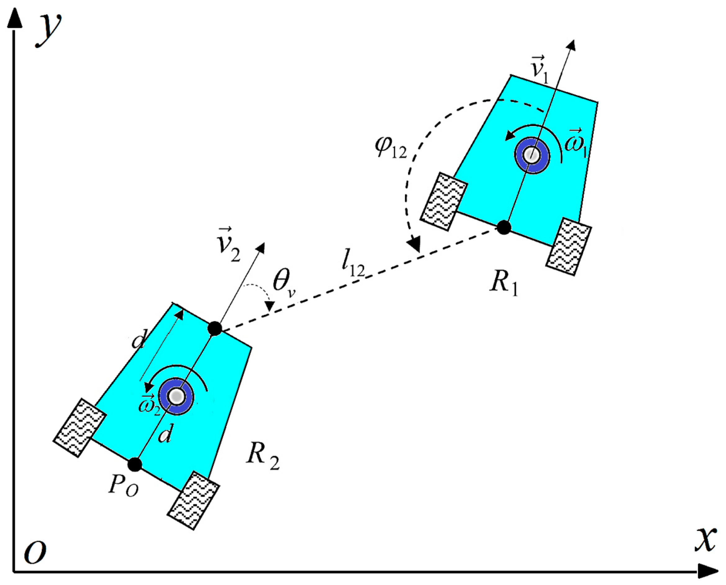
Illustrated in Figure 1 are two robotic entities configured within a leader–follower formation. The follower robot, denoted as $R_2$, demonstrates adherence to the leader robot, designated as $R_1$, maintaining a separation denoted as $l_{12}$ along with a relative orientation marked as ${\phi }_{12}$. Notably, a relative motion sensor is strategically positioned at point C atop robot $R_2$.

Expressed concisely, the kinematic equation for each individual robot takes the subsequent form ($i=\mathrm{1,2}$) [9]:

$$\left(\begin{array}{c}{\dot{x}}_{ci}\\ {\dot{y}}_{ci}\end{array}\right)=\left(\begin{array}{cc}cos{\theta }_i& -dsin{\theta }_i\\ sin{\theta }_i& dcos{\theta }_i\end{array}\right)\left(\begin{array}{c}{v}_i\\ {\omega }_i\end{array}\right),{\dot{\theta }}_i={\omega }_i$$

(1)

where $\left(x_{ci}{y}_{ci}\right)$ symbolizes the coordinates of point C within the broader global coordinate framework, and ${\theta }_i$ signifies the directional angle of the respective robot. As visually depicted in Figure 1, $\overrightarrow{v_i}$ and $\overrightarrow{{\omega }_i}$ denote the linear and angular velocities (respectively, with units m/s and rad/s) associated with robot $R_i$, with their scalar representations manifesting as $v_{\mathrm{i}}$ and ${\omega }_i$, correspondingly.$P_0$ represents the juncture at which the axis of symmetry intersects with the mobile wheel axis, while d quantifies the distance extending from the center of mass to the reference point C.

The distance between two robots can be obtained from the following relationship:

$$l_{12}=\sqrt{{(x_1-x_2)}^2+{(y_1-y_2)}^2}$$

(2)

And the relative direction between two robots is as follows:

$${\phi }_{12}=\pi -{\theta }_{v2}-{\theta }_1+{\theta }_2$$

(3)

where the units of $l_{12}$ and ${\phi }_{12}$ and other distance and angles are, respectively, m and rad throughout this paper. By taking derivatives from these two relationships and using the kinematic equations stated in (1), we have [20,21]

$$M\left(\begin{array}{c}{\dot{l}}_{12}\\ {\dot{\phi }}_{12}\end{array}\right)-N\left(\begin{array}{c}{v}_1\\ {\omega }_1\end{array}\right)=\left(\begin{array}{c}{v}_2\\ {\omega }_2\end{array}\right)$$

(4)

where matrices M and N are defined as follows:

$$M=\left(\begin{array}{cc}-cos{\theta }_{v2}& -l_{12}sin{\theta }_{v2}\\ \left(sin{\theta }_{v2}\right)/d& -\left(l_{12}cos{\theta }_{v2}\right)/d\end{array}\right)$$

$$N=\left(\begin{array}{cc}-cos{\theta }_{12}& l_{12}sin{\theta }_{v2}\\ -\left(sin{\theta }_{12}\right)/d& \left(l_{12}cos{\theta }_{v2}\right)/d\end{array}\right)$$

In this relation, ${\theta }_{12}={\theta }_1-{\theta }_2$ and, as shown in Figure 1, ${\theta }_{v2}=\pi -{\phi }_{12}-{\theta }_{12}$ show the relative direction between the speed, $v_2,$ and the line, $l_{12}$.

By defining the state variables as $q={\left(l_{12}{\phi }_{12}\right)}^T$ and $\dot{q}={\left({\dot{l}}_{12}{\dot{\phi }}_{12}\right)}^T$ and the input of the formation system as $u={\left(v_2{\omega }_2\right)}^T$, we can write Equation (4) in a simplified form as follows:

$$\dot{q}=G\times \left(u+\delta \right)+\eta$$

(5)

where $\eta$ stands for the external disturbances and the G and δ, matrices which are defined as follows:

$$G=M^{-1}=\left(\begin{array}{cc}-cos{\theta }_{v2}& dsin{\theta }_{v2}\\ -sin{\theta }_{v2}/l_{12}& -dcos{\theta }_{v2}/l_{12}\end{array}\right)$$

$$\delta =N\left(l_{12},{\theta }_{12},{\theta }_{v2}\right)\left(\begin{array}{c}{v}_1\\ {\omega }_1\end{array}\right)$$

Note 1. 

The final component, denoted as δ in Equation (5), encapsulates the influence stemming from the absolute velocity of the leader robot. This variable proves challenging to precisely gauge and approximate, owing to the constraints that are inherent to motion sensors, thus representing an inherent uncertainty within the system’s model.

2.1.2. Leader–Leader Formation Kinematic Model

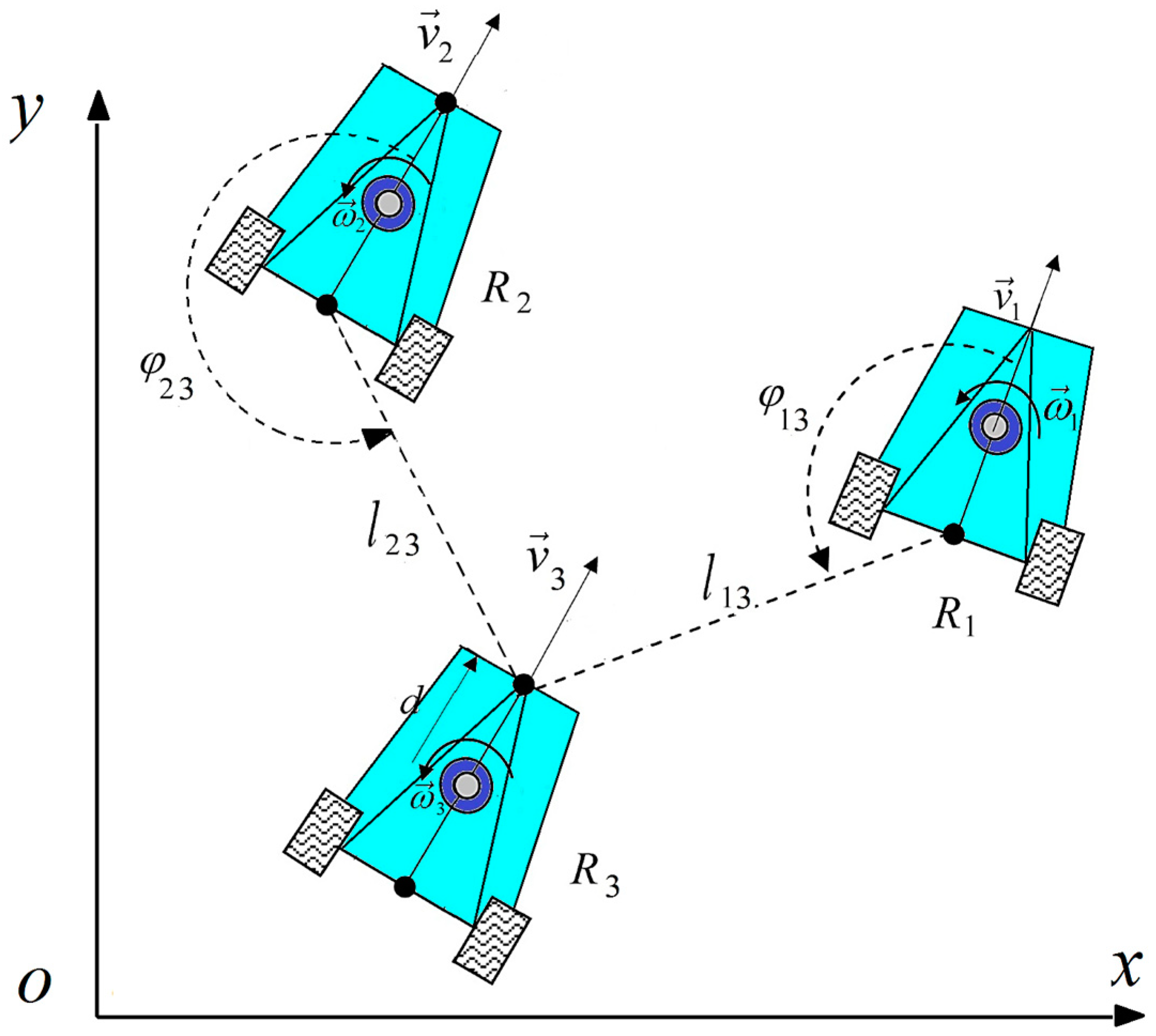
Depicted in Figure 2 is a triad of non-holonomic mobile robots, each with their unique attributes. Within the context of leader–leader formation control (abbreviated as l-l), the objective entails the third robot effectively preserving optimal distances, denoted as  $l_{13}^d$ and $l_{23}^d$, in relation to its two designated leaders. It is obvious that, for this purpose, the two leader robots should never be placed at a distance of more than $l_{13}^d+l_{23}^d$ from each other.

By taking derivatives from Equation (2) for the distance between the two robots $R_1$ and $R_3$ ($l_{13}$) and the distance between the two robots $R_2$ and $R_3$ ($l_{23}$), and using the kinematic equations stated in (1), the following equation as a first-order model for leader–follower formation will be achieved:

$$M\left[\begin{array}{c}{\dot{l}}_{13}\\ {\dot{l}}_{23}\end{array}\right]-N\left[\begin{array}{c}{v}_1\\ v_2\end{array}\right]=\left[\begin{array}{c}{v}_3\\ {\omega }_3\end{array}\right]$$

(6)

where the matrices M and N are defined as follows:

$$M=\frac{1}{dsin\left({\gamma }_2-{\gamma }_1\right)}\left[\begin{array}{cc}dsin\left({\gamma }_2\right)& -dsin\left({\gamma }_1\right)\\ -\mathit{cos}\left({\gamma }_2\right)& \mathit{cos}\left({\gamma }_1\right)\end{array}\right]$$

$$N=\frac{1}{dsin({\gamma }_2-{\gamma }_1)}$$

$$\times \left[\begin{array}{cc}-dcos\left({\phi }_{13}\right)sin\left({\gamma }_2\right)& dsin\left({\gamma }_1\right)cos\left({\phi }_{23}\right)\\ cos\left({\gamma }_2\right)cos\left({\phi }_{13}\right)& -cos\left({\gamma }_1\right)cos\left({\phi }_{23}\right)\end{array}\right]$$

And we have ${\gamma }_i={\theta }_i+{\phi }_{i3}-{\theta }_3(i=\mathrm{1,2})$. By defining the state variables as $q={\left(l_{13}{l}_{23}\right)}^T$ and $\dot{q}={\left({\dot{l}}_{13}{\dot{l}}_{23}\right)}^T$, and the input of the formation system as $u={\left(v_3{\omega }_3\right)}^T,$ Equation (6) is rewritten as follows:

$$\dot{q}=G\times \left(u+\delta \right)+\eta$$

(7)

Such that $\eta$ stands for the disturbance vector and the G and δ matrices are defined as follows:

$$G=M^{-1}=\left[\begin{array}{cc}cos{\gamma }_1& dsin{\gamma }_1\\ cos{\gamma }_2& dsin{\gamma }_2\end{array}\right]$$

$$\delta =N\left[\begin{array}{c}{v}_1\\ v_2\end{array}\right]$$

The ultimate term δ within Equation (7) illustrates the impact stemming from the linear velocity of the leader robots, serving as a representation of the inherent uncertainty that is intrinsic to the system.

2.2. Second-Order Kinematic Model of Formation

2.2.1. Leader–Follower Formation Kinematic Model

In Equation (4), the movement states of the formation in the local frame of the follower robot $R_2$ are depicted. The follower robot has no knowledge of the absolute speed of the leader robot and, as a result, can only estimate the relative speed of the leader robot in respect of itself using motion sensors installed at its front. Equation (4) can be written as

$$N^{-1}\left[M\left(\begin{array}{c}{\dot{l}}_{12}\\ {\dot{\phi }}_{12}\end{array}\right)-\left(\begin{array}{c}{v}_2\\ {\omega }_2\end{array}\right)\right]=\left(\begin{array}{c}{v}_1\\ {\omega }_1\end{array}\right)$$

(8)

Deriving from (4) and combining with (8), we have

$$\begin{gathered} \left(\begin{array}{c}{\dot{v}}_2\\ {\dot{\omega }}_2\end{array}\right)=M\left(\begin{array}{c}{\ddot{l}}_{12}\\ {\ddot{\phi }}_{12}\end{array}\right)+C\left(\begin{array}{c}{\dot{l}}_{12}\\ {\dot{\phi }}_{12}\end{array}\right)-{\dot{\theta }}_{12}\left(\begin{array}{c}h{\omega }_2\\ -v_2/d\end{array}\right) \\ +M\left(\begin{array}{c}-l_{12}{\dot{\phi }}_{12}\\ {\dot{l}}_{12}/l_{12}\end{array}\right){\omega }_2+\left(\begin{array}{c}{\delta }_1\\ {\delta }_2\end{array}\right) \end{gathered}$$

(9)

where matrix C and vector δ are defined as follows:

$$C=\left(\begin{array}{cc}{\dot{\theta }}_{v2}sin{\theta }_{v2}& -{\dot{\theta }}_{v2}{l}_{12}cos{\theta }_{v2}-{\dot{l}}_{12}sin{\theta }_{v2}\\ \left({\dot{\theta }}_{v2}cos{\theta }_{v2}\right)/d& ({\dot{\theta }}_{v2}{l}_{12}sin{\theta }_{v2}-{\dot{l}}_{12}cos{\theta }_{v2})/d\end{array}\right)$$

$$\delta =\left(\begin{array}{c}{\delta }_1\\ {\delta }_2\end{array}\right)=M\left(\begin{array}{c}-{\dot{v}}_{1}cos{\phi }_{12}\\ \frac{{\dot{v}}_{1}sin{\phi }_{12}}{l_{12}}-{\dot{\omega }}_1\end{array}\right)+\left(\begin{array}{c}{\eta }_1\\ {\eta }_2\end{array}\right)$$

where ${\dot{\theta }}_{12}={\omega }_1-{\omega }_2$ and ${\dot{\theta }}_{v2}=-{\dot{\phi }}_{12}-{\dot{\theta }}_{12}$ are used in (9), and ${\left({\eta }_1{\eta }_2\right)}^T$ stands for the bounded external disturbance vector. Note that the state variables with $q={\left(l_{12}{\phi }_{12}\right)}^T$ and $\dot{q}={\left({\dot{l}}_{12}{\dot{\phi }}_{12}\right)}^T$ and the input of the robot formation system with $u={\left({\dot{v}}_2{\dot{\omega }}_2\right)}^T$ are specified. Equation (9) can be rewritten as follows:

$$\begin{gathered} u=M\left(q,{\theta }_{12}\right)\ddot{q}+C\left(q,\dot{q},{\theta }_{12},{\dot{\theta }}_{12}\right)\dot{q} \\ +G\left(q,\dot{q},{\theta }_{12},{\dot{\theta }}_{12},v_2,{\omega }_2\right)+\delta \left({\dot{v}}_1,{\dot{\omega }}_1,q,\dot{q}\right) \end{gathered}$$

(10)

where the function $G\left(q,\dot{q},{\theta }_{12},{\dot{\theta }}_{12},v_2,w_2\right)$ is defined as follows:

$$G=-{\dot{\theta }}_{12}\left(\begin{array}{c}h{\omega }_2\\ -v_2/d\end{array}\right)+M\left(\begin{array}{c}-l_{12}{\dot{\phi }}_{12}\\ {\dot{l}}_{12}/l_{12}\end{array}\right){\omega }_2$$

(11)

Equation (10) establishes the interconnection between inputs and outputs within the leader–follower robot formation framework. The outputs encompass relative metrics such as the distance, direction, and velocities between the robots, while the inputs correspond to the follower robot’s absolute accelerations within local coordinates. The relative motion states $q$, $\dot{q},$ and ${\dot{\theta }}_{12}$, delineated in Equation (10), can be conveniently assessed using the relative motion sensors that are embedded in the follower robot.

Note 2. 

The incorporation of the second-order kinematic model (10) results in a multi-variable, non-linear system configuration. This facet facilitates a more comprehensive scrutiny of the control system’s effectiveness, enabling the formulation of non-linear control strategies that ensure holistic stability. Moreover, this model opens avenues for pursuing intricate trajectory tracking, transcending the capabilities of the first-order kinematic model.

Note 3. 

Exploiting Equation (10), the centripetal accelerations and Coriolis effect, denoted as $C\dot{q}+G$within (10), can be directly computed utilizing the outcomes furnished with both the relative motion sensors and the local motion sensor mounted on the follower robot. Furthermore, these relative accelerations serve to linearize the intricate nonlinear dynamics that are inherent to the leader–follower formation setup.

Note 4. 

The ultimate term δ presented within Equation (10) encapsulates the influence originating from the leader robot’s absolute acceleration. This parameter proves to be intricate to precisely measure and gauge, owing to the inherent limitations of motion sensors, and consequently represents a quintessential component of the system’s model uncertainty.

2.2.2. Leader–Leader Formation Kinematic Model

Through the resolution of Equation (6), the absolute linear velocity of the leader robots, a quantity beyond the capacity of measurement by the obstacle robot, is formulated in terms of the formation’s motion states and the absolute velocity of the follower robot, as delineated below:

$$\left[\begin{array}{c}{v}_1\\ v_2\end{array}\right]=N^{-1}\left[M\left[\begin{array}{c}{\dot{l}}_{13}\\ {\dot{l}}_{23}\end{array}\right]-\left[\begin{array}{c}{v}_3\\ {\omega }_3\end{array}\right]\right]$$

(12)

By taking the derivative from (6) and combining with (12), we have:

$$\left[\begin{array}{c}{\dot{v}}_3\\ {\dot{\omega }}_3\end{array}\right]=M\left[\begin{array}{c}{\ddot{l}}_{13}\\ {\ddot{l}}_{23}\end{array}\right]+C\left[\begin{array}{c}{\dot{l}}_{13}\\ {\dot{l}}_{23}\end{array}\right]-C^{\mathrm{’}}\left[\begin{array}{c}{v}_1\\ v_2\end{array}\right]+\left[\begin{array}{c}{\delta }_1\\ {\delta }_2\end{array}\right]$$

(13)

where the matrices $C$ and $C^{\prime }$ have not been calculated due to the large amount of calculations and the vector $\delta$ is defined as follows:

$$\delta =\left[\begin{array}{c}{\delta }_1\\ {\delta }_2\end{array}\right]=-N\left[\begin{array}{c}{\dot{v}}_1\\ {\dot{v}}_2\end{array}\right]+\left(\begin{array}{c}{\eta }_1\\ {\eta }_2\end{array}\right)$$

where ${\left({\eta }_1{\eta }_2\right)}^T$ stands for the bounded external disturbance vector. We now define the state variables as follows:

$$q={\left[l_{13}\hspace{1em}{l}_{23}\right]}^T$$

$$\dot{q}={\left[{\dot{l}}_{13}\hspace{1em}{\dot{l}}_{23}\right]}^T$$

and the input of the robot formation system is specified as $u={\left[{\dot{v}}_3{\dot{\omega }}_3\right]}^T$. Equation (13) can be rewritten as follows:

$$\begin{gathered} u=M\left({\gamma }_1,{\gamma }_2\right)\ddot{q}+C\left({\gamma }_1,{\gamma }_2,{\dot{\gamma }}_1,{\dot{\gamma }}_2\right)\dot{q} \\ +G\left({\gamma }_1,{\gamma }_2,\dot{q},v_3,{\omega }_3\right)+\delta \left({\gamma }_1,{\gamma }_2,{\dot{v}}_1,{\dot{v}}_2\right) \end{gathered}$$

(14)

where the function $G\left({\gamma }_1,{\gamma }_2,\dot{q},v_3,{\omega }_3\right)$ is defined as follows:

$$G=-C^{\prime }\left[\begin{array}{c}{v}_1\\ v_2\end{array}\right]$$

Equation (14) establishes the interplay between inputs and outputs within the leader–leader formation system under the $l-l$ mode. The outputs encompass the relative metrics, specifically the distances and velocities between the robots. In this context, the inputs comprise the absolute accelerations originating from the follower robot’s local coordination. The relative motion states $q$ and $\dot{q}$, featured in Equation (12), are determined through the utilization of the relative motion sensors positioned on the follower robot.

Note 5. 

Analogous to the leader–follower formation setup, the ultimate term δ presented within Equation (14) signifies the impact arising from the linear acceleration of the leader robots. This parameter proves to be intricate to precisely measure and gauge due to the limitations that are inherent in motion sensors, thereby representing a core element of uncertainty within the system’s model.

Note 6. 

Equations (10) and (14) both have the same structure and, as we will see in next section, the stabilizing controller is same for both models. The designed controller should provide the linear acceleration  ${(\dot{v}}_3)$ and angular acceleration  $\left({\dot{\omega }}_3\right)$ of the follower robot in such a way that, despite keeping the formation, the system stays robust against the disturbances and uncertainties of the model and input constraints, and in addition, model matrices are not used in the controller structure.

3. Design of Robust Adaptive Controller

In this section, at first, a controller will be designed, taking into account the uncertainties and unknown dynamics of modeling in the first-order formation and assuming that there is no knowledge about the upper band of uncertainty, so that the follower robot will be placed at the optimal distance and angle to the leader. In the following, according to the second-order formation models, a robust adaptive controller will be designed to deal with uncertainties and unknown dynamics in the model. In this controller, the unknown parameters of the arrangement model are estimated in the form of an adaptation law.

3.1. Robust Adaptive Controller for First-Order Model of Formation

In this section, the design of the controller is performed based on the leader–follower first-order formation model, which is given in Equation (5). The controller design for the leader–leader formation in Equation (7) is quite similar.

First, we rewrite Equation (5) as follows:

$$\dot{q}=G\times u+d$$

(15)

where $d=G\times \delta +\eta$ is considered as the uncertainty and disturbance of the system.

Assume that the uncertainty is limited as $‖d‖\le \gamma$ and we have no information about the upper band of $\gamma$. After estimating it, we use it as $\overline{\gamma }$ in the design of the controller. In this case, consider $‖.‖$ as the absolute value of the vector entries, meaning that $‖d‖={(\left|d_1\right|,\left|d_2\right|)}^{\mathrm{T}}$. Also, $\gamma ={({\gamma }_1,{\gamma }_2)}^{\mathrm{T}}$ and $‖d‖\le \gamma$ means $\left|d_1\right|\le {\gamma }_1$ and $\left|d_2\right|\le {\gamma }_2$.

Remark. 

The units of some variables in the first-order model in Equation (15) and in the second-order model in Equation (21) can be surmised in the following table (

Table 1. Units of variables in this study.

Variable	Unit	Variable	Unit
$q={\left(l_{12}{\phi }_{12}\right)}^T$	${(\mathrm{m},\mathrm{r}\mathrm{a}\mathrm{d})}^{\mathrm{T}}$	$u={\left({\dot{v}}_3{\dot{\omega }}_3\right)}^T$	${\left(\mathrm{m}/{\mathrm{s}}^2\mathrm{r}\mathrm{a}\mathrm{d}/{\mathrm{s}}^2\right)}^{\mathrm{T}}$
$q={\left(l_{13}{l}_{23}\right)}^T$	${(\mathrm{m},\mathrm{m})}^{\mathrm{T}}$	$d={(d_1,d_2)}^T$ in (15) for $l-l$ model	${\left(\mathrm{m}/\mathrm{s},\mathrm{m}/\mathrm{s}\right)}^{\mathrm{T}}$
$\dot{q}={\left({\dot{l}}_{12}{\dot{\phi }}_{12}\right)}^T$	${(\mathrm{m}/\mathrm{s},\mathrm{r}\mathrm{a}\mathrm{d}/\mathrm{s})}^{\mathrm{T}}$	$d={(d_1,d_2)}^T$ in (15) for $l-\phi$ model	${(\mathrm{m}/\mathrm{s},\mathrm{r}\mathrm{a}\mathrm{d}/\mathrm{s})}^{\mathrm{T}}$
$\dot{q}={\left({\dot{l}}_{12}{\dot{l}}_{23}\right)}^T$	${(\mathrm{m}/\mathrm{s},\mathrm{m}/\mathrm{s})}^{\mathrm{T}}$	${\delta }_i$ in (21) for $l-l$ model	${\left(\mathrm{m}/{\mathrm{s}}^2\mathrm{m}/{\mathrm{s}}^2\right)}^{\mathrm{T}}$
$u={\left(v_2{\omega }_2\right)}^T$	${\left(\mathrm{m}/\mathrm{s}\mathrm{r}\mathrm{a}\mathrm{d}/\mathrm{s}\right)}^{\mathrm{T}}$	${\delta }_i$ in (21) for $l-\phi$ model	${\left(\mathrm{m}/{\mathrm{s}}^2\mathrm{r}\mathrm{a}\mathrm{d}/{\mathrm{s}}^2\right)}^{\mathrm{T}}$

). Note that the units of these variables according to the leader–leader (denoted as  $l-l$) and leader–follower models (denoted as $l-\phi$) are different.

Note 7. 

It should be noted in the leader–follower model that the term $\delta$ includes  $v_1$ and  ${\omega }_1,$ and in the leader–leader model  $\delta$ includes  $v_1$ and  $v_2$. Now, given that measuring the absolute velocities of leaders is very difficult for the follower robot due to the constraints of the motion sensors (the follower robot can only measure its relative velocity with leaders and not the absolute velocity of leaders), then the term  $\delta$ is considered as the modeling uncertainty in (15). In the equation  $d=G\times \delta +\eta$, $\delta$ stands for uncertainties and  $\eta$ stands for disturbances, and therefore the term  $d$ can be called system perturbation, which can be defined as a summation of the undertrained terms ($G\times \delta$) and disturbances ($\eta$) of the system.

We write Equation (15) with the definition $\tilde{q}=q-q_d$ as follows:

$$\dot{\tilde{q}}=Gu+d-{\dot{q}}_d$$

(16)

where $q_d=[l_{12}^d,{\phi }_{12}^d]$ shows the optimal values of the distance and angle of the follower robot relative to the leader robot.

Theorem 1. 

Consider Equation (5). In this case, the control input is

$$u=G^{-1}\left\{-\mathsf{\Lambda }\tilde{q}+{\dot{q}}_d\right\}-\overline{\gamma }$$

(17)

where $\overline{\gamma }$  is estimated using the following adaptive law,

$$\dot{\overline{\gamma }}=G^T\tilde{q}-\tilde{q}$$

(18)

and $\mathsf{\Lambda }$ is a positive definite matrix; it will cause the states $q=[l_{12},{\phi }_{12}]$ to converge to the desired values $q_d=\left[l_{12}^d,{\phi }_{12}^d\right]$ in the closed-loop system.

Proof: 

Consider the Lyapunov function, as below:

$$V=\frac{1}{2}{\tilde{q}}^T\tilde{q}+\frac{1}{2}{\tilde{\gamma }}^T\tilde{\gamma }$$

(19)

in which $\tilde{\gamma }=\overline{\gamma }-\gamma ,$ and $V$ is a positive definite value. By taking the time derivative from (19) and using Equations (16) and (17), we have

$$\begin{gathered} \dot{V}={\tilde{q}}^T\dot{\tilde{q}}+{\tilde{\gamma }}^T\dot{\tilde{\gamma }}={\tilde{q}}^T\left(-\mathsf{\Lambda }\tilde{q}-G\overline{\gamma }+d\right)+{\tilde{\gamma }}^T\dot{\tilde{\gamma }} \\ =-{\tilde{q}}^T\mathsf{\Lambda }\tilde{q}-{\tilde{q}}^{T}G\overline{\gamma }+{\tilde{q}}^{T}d+{\overline{\gamma }}^T\dot{\overline{\gamma }} \\ \le -{\tilde{q}}^T\mathsf{\Lambda }\tilde{q}-{\tilde{q}}^{T}G\overline{\gamma }+{\tilde{q}}^T\overline{\gamma }+{\overline{\gamma }}^T(G^T\tilde{q}-\tilde{q}) \end{gathered}$$

(20)

Considering the equality of ${\tilde{q}}^{T}G\overline{\gamma }$ and ${\overline{\gamma }}^T{G}^T\tilde{q}$ (because both are scalars), and also ${\tilde{q}}^T\overline{\gamma }$ and ${\overline{\gamma }}^T\tilde{q}$ using Equation (18), we have:

$$\dot{V}\le -{\tilde{q}}^T\mathsf{\Lambda }\tilde{q}$$

Which, according to the positive definiteness of $\mathsf{\Lambda },$ we have:

$$\tilde{q}\to 0\Rightarrow q\to q_d$$

□

Note 8. 

The robust adaptive control method which is mentioned in this section can be proven in the case of the leader–leader formation, which will not be repeated again in order to avoid repetition. The formation control law in (17) and (18) can easily be applied for the leader–leader formation model in (7) without the loss of generality, and the only difference is that, for the leader–leader case, we should consider G and δ as in model (7) and $q$ and  $q_d$ as  $q={\left(l_{13}{l}_{23}\right)}^T$ and  $q_d={\left(l_{13}^d{l}_{23}^d\right)}^T$ to achieve leader–leader formation.

3.2. Robust Adaptive Controller for the Second-Order Model

In this section, the design of the controller is carried out based on the second-order kinematic models in (10) and (14). In the second-order models, the accelerations of the leader robots are also included in the equations. The goal is to design the controller in such a way that, in the presence of uncertainty and disturbance and without using model matrices, the follower robot can be made to maintain the formation.

In Equations (10) and (14), the goal is to design the controller $u$ in such a way that $q_i\to q_{desi}$, where $i=\mathrm{1,2}$. For the leader–follower model in (10), we have $i=1$ and $q_{des1}={\left(l_{12}^d{\phi }_{12}^d\right)}^T,$ and for the leader–leader model in (14), we have $i=2$ and $q_{des2}={\left(l_{13}^d{l}_{23}^d\right)}^T$. In order to design the controller, we use the following model, which corresponds to both the leader–follower and leader–leader formation models:

$$M_i\left(q_i\right){\ddot{q}}_i+C_i\left(q_i,{\dot{q}}_i\right){\dot{q}}_i+G_i+{\delta }_i=u_i$$

(21)

Note 9. 

In the leader–follower model, the uncertain term $\delta$ is the summation of the leader’s linear and angular accelerations  $\left(\begin{array}{c}{\dot{v}}_1\\ {\dot{\omega }}_1\end{array}\right)$ (which are not easy for the follower robot to measure) and the external disturbances $\left(\begin{array}{c}{\eta }_1\\ {\eta }_2\end{array}\right)$. Also, in the leader–leader formation model,  $\delta$ is the summation of the terms of the leader 1 and leader 2 linear accelerations  $\left[\begin{array}{c}{\dot{v}}_1\\ {\dot{v}}_2\end{array}\right]$ (which are also very difficult for the followers to measure) and the external disturbances  $\left(\begin{array}{c}{\eta }_1\\ {\eta }_2\end{array}\right)$. The unknown term  $\delta$, which is a sumation of uncertainties and disturbances, can be defined as system perturbation.

Now, with the definition of $e_i=q_{di}-q_i$, where $q_{di}$ shows the desired formation for each of the follower robots in both models, and with the definition of $r_i=e_i+{\dot{e}}_i$, the robust adaptive controller for the i-th model will be in the following form [22]:

$$u_i=K_{iv}{r}_i+V_{iR}$$

(22)

In this relation, $K_{iv}$ is a positive definite diagonal and square matrix, and we have

$$V_{iR}=\frac{r_i{\widehat{\rho }}_i^2}{{\widehat{\rho }}_i‖r_i‖+{\epsilon }_i}$$

(23)

where the scalar, ${\epsilon }_i,$ is obtained from the following relation:

$${\dot{\epsilon }}_i=-K_{\epsilon }{\epsilon }_i,{\epsilon }_i\left(0\right)=1,K_{\epsilon }\in {\mathcal{R}}^{+}$$

(24)

and the scalar function, ${\widehat{\rho }}_i,$ is obtained from the following equation:

$${\widehat{\rho }}_i=s_i{\widehat{\theta }}_i$$

(25)

$$s_i=\left(\begin{array}{ccc}1& ‖e_i‖& {‖e_i‖}^2\end{array}\right)$$

(26)

$${\widehat{\theta }}_i={\left(\begin{array}{ccc}{\widehat{\delta }}_0& {\widehat{\delta }}_1& {\widehat{\delta }}_2\end{array}\right)}^T$$

(27)

Here, $s_i$ is the regressor matrix and ${\widehat{\theta }}_i$ is the parameter estimator vector. The adaptive law that estimates the unknown parameters is in the following form:

$${\dot{\widehat{\theta }}}_i={\gamma }_i{s}_i^T‖r_i‖$$

(28)

In this law, ${\gamma }_i$ is an arbitrary positive constant.

Theorem 2. 

By applying the control law (22), the formation error in both the leader–follower and leader–leader models in (21) converges to zero, and the estimated parameters in (28) will also remain limited.

Proof: 

The stability proof of applying the formation controller (22) into the formation model in (21) is similar to the proof given in [22], which is presented for applying a controller with a similar structure to that of (22), which was used for solving the desired path tracking problem using a model of mechanical arms, similar to the model in (21).

We assume that the dynamics given below show uncertainty for the follower controller in the i-th model [22].

$$\begin{gathered} w_i=M_i\left(q_i\right)\left({\ddot{q}}_d+{\dot{e}}_i\right)+C_i\left(q_i,{\dot{q}}_i\right)\left({\dot{q}}_d+e_i\right) \\ +G_i+{\delta }_i \end{gathered}$$

(29)

Suppose that a scalar function like ${\rho }_i$ can be used to limit this uncertain dynamic.

$${\rho }_i\ge ‖w_i‖$$

(30)

The unknown dynamics of $w_i$ can be limited as follows:

$${\rho }_i={\delta }_0+{\delta }_1‖e_i‖+{\delta }_2{‖e_i‖}^2\ge ‖w_i‖$$

(31)

In relation (31), parameters ${\delta }_0$, ${\delta }_1,$ and ${\delta }_2$ are limited and positive constants. According to the relations ${\dot{e}}_i={\dot{q}}_d-{\dot{q}}_i$ and ${\ddot{e}}_i={\ddot{q}}_d-{\ddot{q}}_i,$ and increasing and decreasing the expressions $M_i{\ddot{q}}_d$ and $C_i{\dot{q}}_d$ in the formation model (21), we have

$$u_i=-M_i{\ddot{e}}_i-C_i{\dot{e}}_i+M_i{\ddot{q}}_d+C_i{\dot{q}}_d+G_i+{\delta }_i$$

(32)

In order to achieve relation (29) again, by adding and subtracting other similar terms, we will reach the following relation:

$$u_i=-M_i{\dot{r}}_i-C_i{r}_i+w_i$$

(33)

where we have ${\dot{r}}_i={\ddot{e}}_i+{\dot{e}}_i$. By applying the proposed controller in (22), Equation (33) will be as follows:

$$M_i{\dot{r}}_i=-C_i{r}_i-K_{iv}{r}_i-V_{iR}+w_i$$

(34)

Now we define the proposed Lyapunov function for the i-model as follows:

$$V_i=\frac{1}{2}{r}_i^T{M}_i{r}_i+\frac{1}{2}{\tilde{\theta }}_i^T{\gamma }_i^{-1}{\tilde{\theta }}_i+K_{\epsilon }^{-1}{\epsilon }_i$$

(35)

By taking the derivative from (35), we have

$$\begin{gathered} {\dot{V}}_i=\frac{1}{2}{r}_i^T{\dot{M}}_i{r}_i+r_i^T{M}_i{\dot{r}}_i+{\tilde{\theta }}_i^T{\gamma }_i^{-1}{\dot{\tilde{\theta }}}_i \\ +K_{\epsilon }^{-1}{\dot{\epsilon }}_i \end{gathered}$$

(36)

Given the system parameters in the parameter vector, ${\theta }_i={\left(\begin{array}{ccc}{\delta }_0& {\delta }_1& {\delta }_2\end{array}\right)}^T$ in (25) and (26), meaning that ${\delta }_0$, ${\delta }_1,$ and ${\delta }_2$ are some scalar and constant values which are invariant with time, so ${\dot{\theta }}_i=0$. Therefore, deriving from the relation ${\tilde{\theta }}_i={\theta }_i-{\widehat{\theta }}_i$ in (36), it can be concluded that

$${\dot{\tilde{\theta }}}_i=-{\dot{\widehat{\theta }}}_i$$

(37)

By substituting Equations (28), (37), and (34) in Equation (36) and simplifying, we will have

$$\begin{gathered} {\dot{V}}_i=\frac{1}{2}{r}_i^T\left({\dot{M}}_i-2C_i\right)r_i-r_i^T{K}_{iv}{r}_i-r_i^T{V}_{iR} \\ +r_i^T{w}_i-s_i{\tilde{\theta }}_i‖r_i‖+K_{\epsilon }^{-1}{\dot{\epsilon }}_i \end{gathered}$$

(38)

By using the property of antisymmetry, the term $\frac{1}{2}{r}_i^T\left({\dot{M}}_i-2C_i\right)r_i$ becomes zero, and by using Equations (25) and (30) and also the property of vector norms $a^{T}b\le ‖a‖‖b‖,$ we will have

$${\dot{V}}_i\le -r_i^T{K}_{iv}{r}_i-r_i^T{V}_{iR}-s_i{\tilde{\theta }}_i‖r_i‖+s_i{\theta }_i‖r_i‖+K_{\epsilon }^{-1}{\dot{\epsilon }}_i$$

(39)

By replacing ${\widehat{\theta }}_i={\theta }_i-{\tilde{\theta }}_i$, and substituting (23) and (24) into (39), we will have

$${\dot{V}}_i\le -r_i^T{K}_{iv}{r}_i-r_i^T\frac{r_i{\widehat{\rho }}_i^2}{{\widehat{\rho }}_i‖r_i‖+{\epsilon }_i}+s_i{\widehat{\theta }}_i‖r_i‖-K_{\epsilon }^{-1}{K}_{\epsilon }{\epsilon }_i$$

(40)

After simplifying and taking the common denominator in the terms on the left, we have

$${\dot{V}}_i\le -r_i^T{K}_{iv}{r}_i-{\epsilon }_i+\frac{{\epsilon }_i\left(s_i{\widehat{\theta }}_i\right)‖r_i‖}{s_i{\widehat{\theta }}_i‖r_i‖+{\epsilon }_i}$$

(41)

The summation $-{\epsilon }_i+\frac{{\epsilon }_i\left(s_i{\widehat{\theta }}_i\right)‖r_i‖}{s_i{\widehat{\theta }}_i‖r_i‖+{\epsilon }_i}$ is always smaller than zero, so the derivative of the proposed Lyapunov function for the i-th model becomes negative.

$${\dot{V}}_i\le -r_i^T{K}_{iv}{r}_i$$

(42)

Now we can consider a new upper band for ${\dot{V}}_i$, such that, using the following relation,

$${\lambda }_{min}\left(K_{iv}\right){‖r_i‖}^2\le r_i^T{K}_{iv}{r}_i\le {\lambda }_{max}\left(K_{iv}\right){‖r_i‖}^2$$

(43)

can write

$${\dot{V}}_i\le -{\lambda }_{min}\left(K_{iv}\right){‖r_i‖}^2$$

(44)

Therefore, ${\dot{V}}_i$ will always be negative definite, and $r_i$ will decrease in this region and tends towards $\epsilon$. In this part, the signals are limited and the signal $r$ is a member of the space $r_i\in L_2^n$. As it has been said, the value of the estimated parameters ${\widehat{\theta }}_i$ and ${\dot{e}}_i$ are also limited. □

Note 10. 

Note that the robust adaptive formation control designed for the first-order formation kinematic model in (15) is robust to the presence of uncertainty,  $G\times \delta$, and disturbance,  $\eta$ (which we called the sum of uncertainty and disturbance as perturbation named  $d=G\times \delta +\eta$). The parameter  $\overline{\gamma }$ in controller (17) is the estimation of the upper bound of perturbation, meaning that  $\gamma$ in  $‖d‖\le \gamma$ and is obtained from the stable adaptive law in (18). The designed robust adaptive control law in (17), according to the proof of stability made using Lyapunov’s theorem in (19) and (20), guarantees the formation in the presence of perturbation, which, not only do we not know, but we also do not know about its upper bound.

Note 11. 

Also, the robust adaptive control law designed for the second-order kinematic formation model in (21) is also robust against perturbation,  ${\delta }_i$. Parameter  ${\widehat{\rho }}_i$ , which is present in the controllers of Equations (22) and (23), is the estimate of the upper band of perturbation in (30), like  ${\rho }_i\ge ‖w_i‖,$ and is obtained from Equation (25) and, as a result, via adaptive law (28). This robust adaptive control law, considering the proof of stability made using Lyapunov’s theorem in Theorem 1, establishes the formation not only in the presence of perturbation but also without any knowledge of the system’s matrices.

3.3. Leader–Obstacle Formation Control

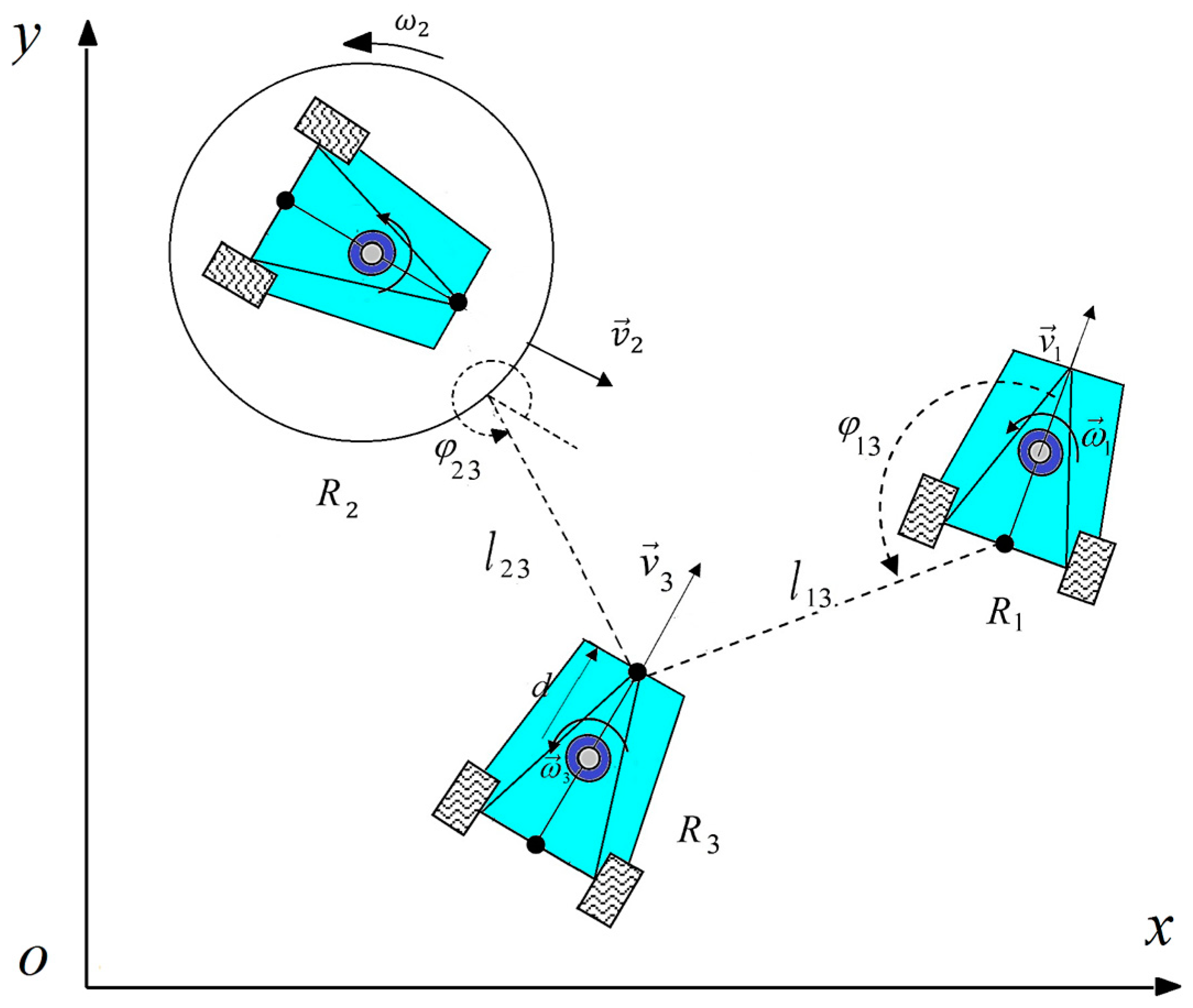
A significant challenge within the control of leader–follower mobile robot formation revolves around safeguarding the follower robot against collisions with dynamic obstacles, while simultaneously maintaining the designated formation alongside the leader robot. In the context of the leader–leader formation model outlined in Equation (14), this challenge is addressed by conceptualizing the obstacle as a virtual leader, thus giving rise to the leader–obstacle formation framework (depicted in Figure 3). In this paradigm, the primary objective involves orchestrating the follower robot, denoted as $R_3$, to track the leader robot $R_1$ while preserving the desired distance, $l_{13}^d$, and concurrently maintaining a predetermined separation from the accelerated moving obstacle, a span indicated as $l_{23}^d$.

In order to have an applicable dynamic obstacle avoidance, there should be a predefined scenario for the follower robot. In this scenario, the formation system, particularly the follower robot, necessitates the integration of a switching mechanism. This mechanism ensures that, as soon as the follower robot detects the presence of an obstacle, it seamlessly transitions its formation strategy from leader–follower to leader–obstacle. To achieve this, strategies like control graphs or the supervisory control of discrete event systems [23], or time-varying switching topologies [27], can be employed. Upon the obstacle’s relocation, and once it exits the follower robot’s visual scope, the formation mode transitions back from leader–obstacle to leader–follower, allowing the follower robot to reestablish alignment with the leader robot.

By implementing the control laws expressed in Equations (17) and (22), the leader–obstacle formation structure can be effectively established, even when confronted with model uncertainties and unfamiliar dynamics.

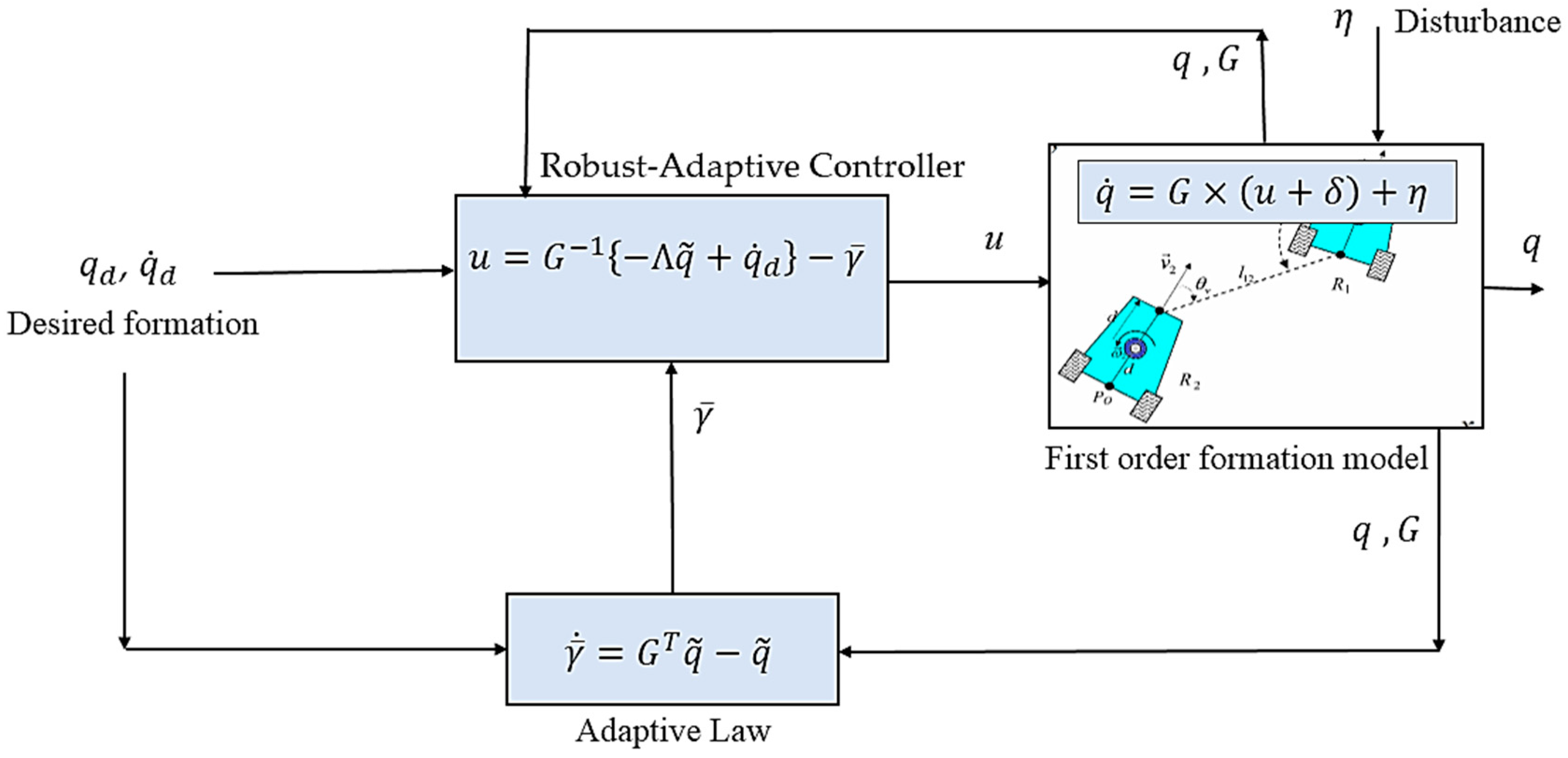
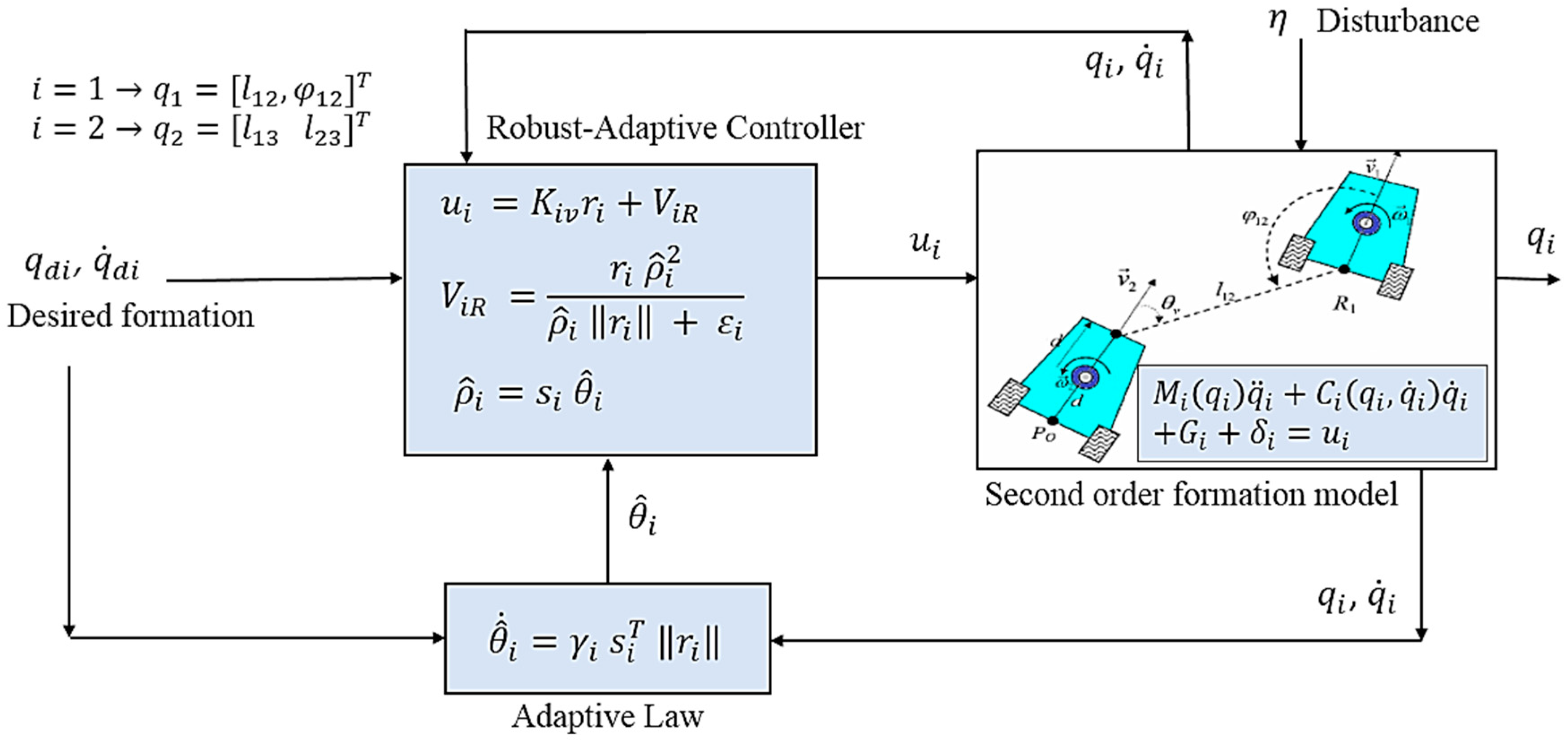
At the end of this section, in order to better understand the methodology presented in this paper, the complete robust adaptive control systems that are proposed in this section to achieve leader–follower and leader–leader formations are presented in the form of block diagrams in Figure 4 and Figure 5. The robust adaptive controller blocks in the first-order formation model in Figure 4 and second-order formation model in Figure 5, respectively, provide the linear and angular velocity (input of the first-order formation model) and linear and angular acceleration (input of the second-order formation model) for the follower robot.

As we can also see from the block diagrams, the adaptive law in Figure 4 estimates the upper bound of disturbance and uncertainties, which is a parameter for control law. In Figure 5, this adaptive law estimates the parameters of the repressor form of the upper bound of the uncertain dynamics, as in (25), (27), and (30).

It is also worth mentioning that the input controller in Figure 4 uses some parts of the formation model, meaning matrix G (which is defined after Equation (5) in the leader–follower model and after Equation (7) in leader–leader model), which includes some parameters of the formation model. However, the robust adaptive controller in Figure 5, as it is clear, only uses variables $q_i$ and ${\dot{q}}_i$, meaning that it does not use any part of the formation model. Therefore, the robust adaptive formation controller in Figure 5 is also said to be model-free to some extent.

4. Simulation Results

This section will showcase the outcomes derived from the implementation of robust adaptive controllers, specifically tailored for the leader–follower formation configuration within mobile robots. These results will be demonstrated through simulation within the MATLAB environment.

4.1. First Simulation Example

In the first simulation, the robust adaptive control law (17) will be applied to a leader–follower formation system. We define the desired state of the system as follows:

$$q_{des}={[l_{12}^d,{\phi }_{12}^d]}^T={[200,\frac{2\pi }{3}]}^T$$

We consider the controller parameter as follows:

$$\mathsf{\Lambda }=\left[\begin{array}{cc}10& 0\\ 0& 10\end{array}\right]$$

(45)

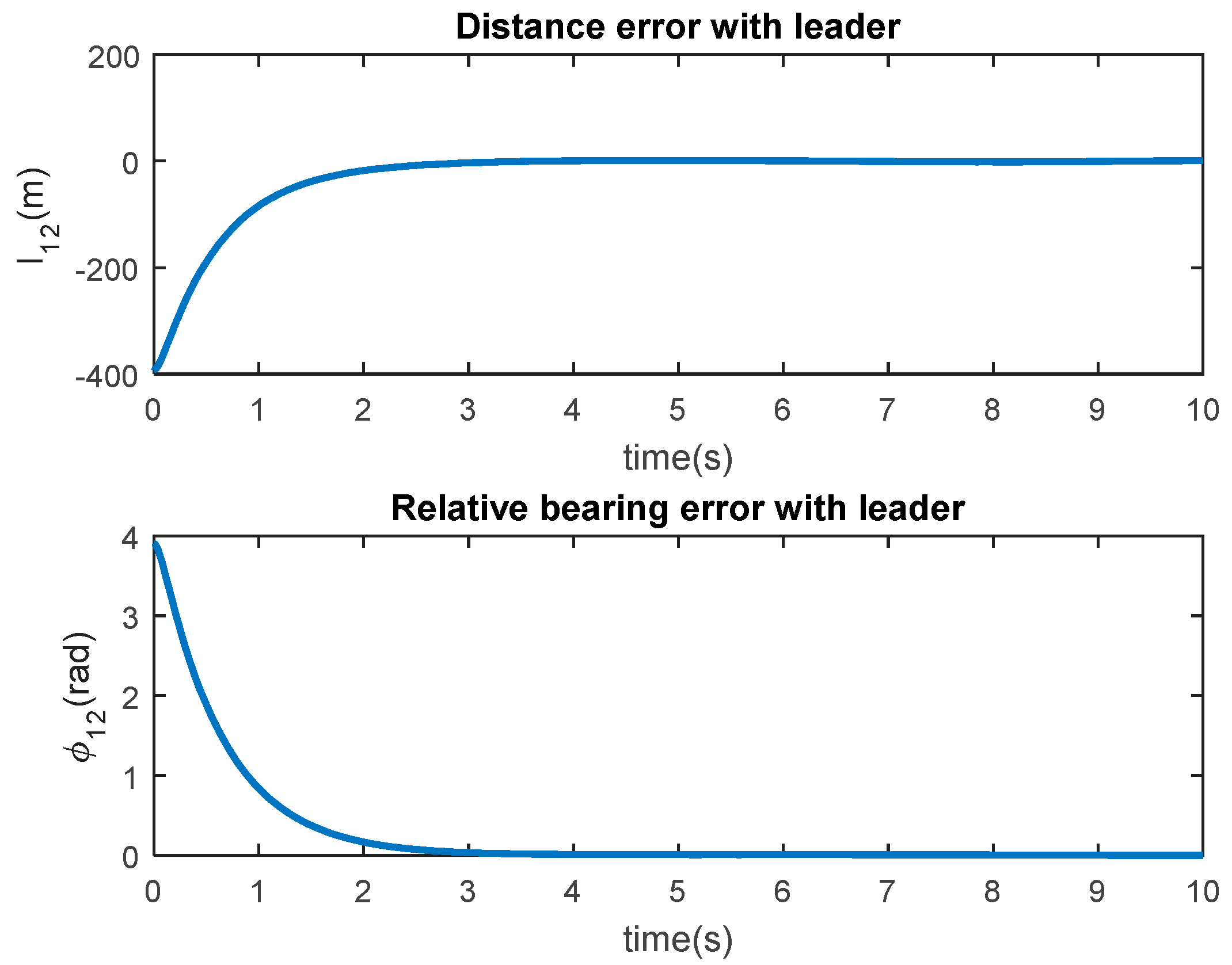
By applying controller (17), the distance and relative orientation errors are shown in Figure 6. As we can see, the relative distance and relative orientation errors between the leader and the follower robot converge to zero, and as a result, the follower robot will follow the leader robot with the desired formation.

In addition, the estimated uncertainty is also shown in Figure 7, and as we can see, this parameter is converged.

4.2. Second Simulation Example

In the second simulation, the robust adaptive control law (22) will be applied to a leader–follower formation system. The simulation results show that the designed controller works well for both the leader–follower and leader–obstacle formations. First, we consider the leader–follower formation. We define the desired state of the system as follows:

$$q_{des}={[l_{12}^d,{\phi }_{12}^d]}^T={[400,\frac{2\pi }{3}]}^T$$

(46)

We consider the controller parameters as follows:

$$\begin{gathered} K_{v1}=\left[\begin{array}{cc}1& 0\\ 0& 2\end{array}\right],k_{\epsilon 1}=1,{\gamma }_1=4 \\ {\widehat{\theta }}_1\left(0\right)={\left[\mathrm{1,2},3\right]}^T,{\epsilon }_1\left(0\right)=1 \end{gathered}$$

(47)

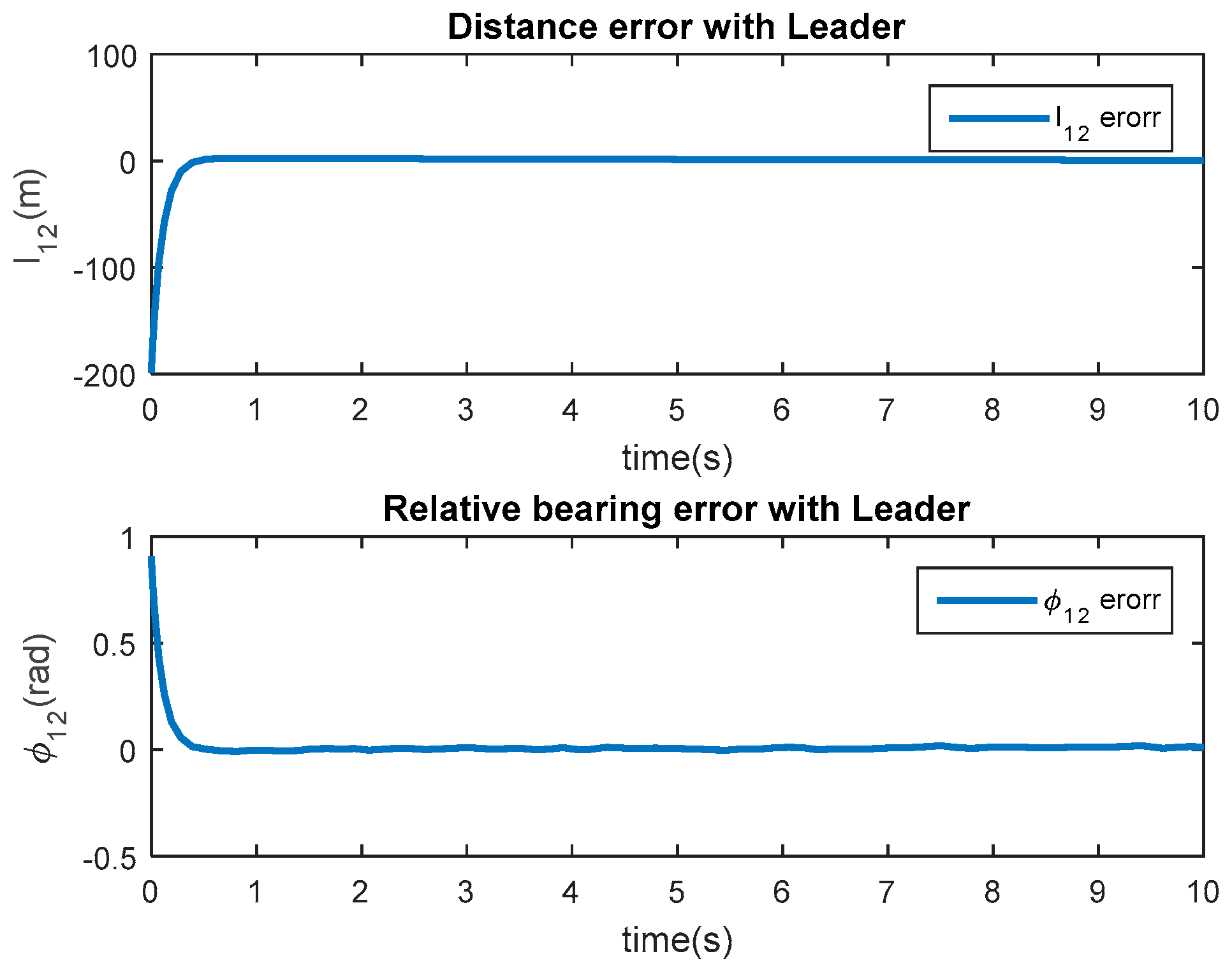
Upon the application of controller (22), the ensuing Figure 8 illustrates the evolution of the distance and relative orientation errors. Notably, the controller’s implementation precipitates the convergence of both the relative distance and relative orientation errors to zero. Consequently, the follower robot achieves a state of conformity, trailing the leader robot, while adhering to the stipulated formation criteria.

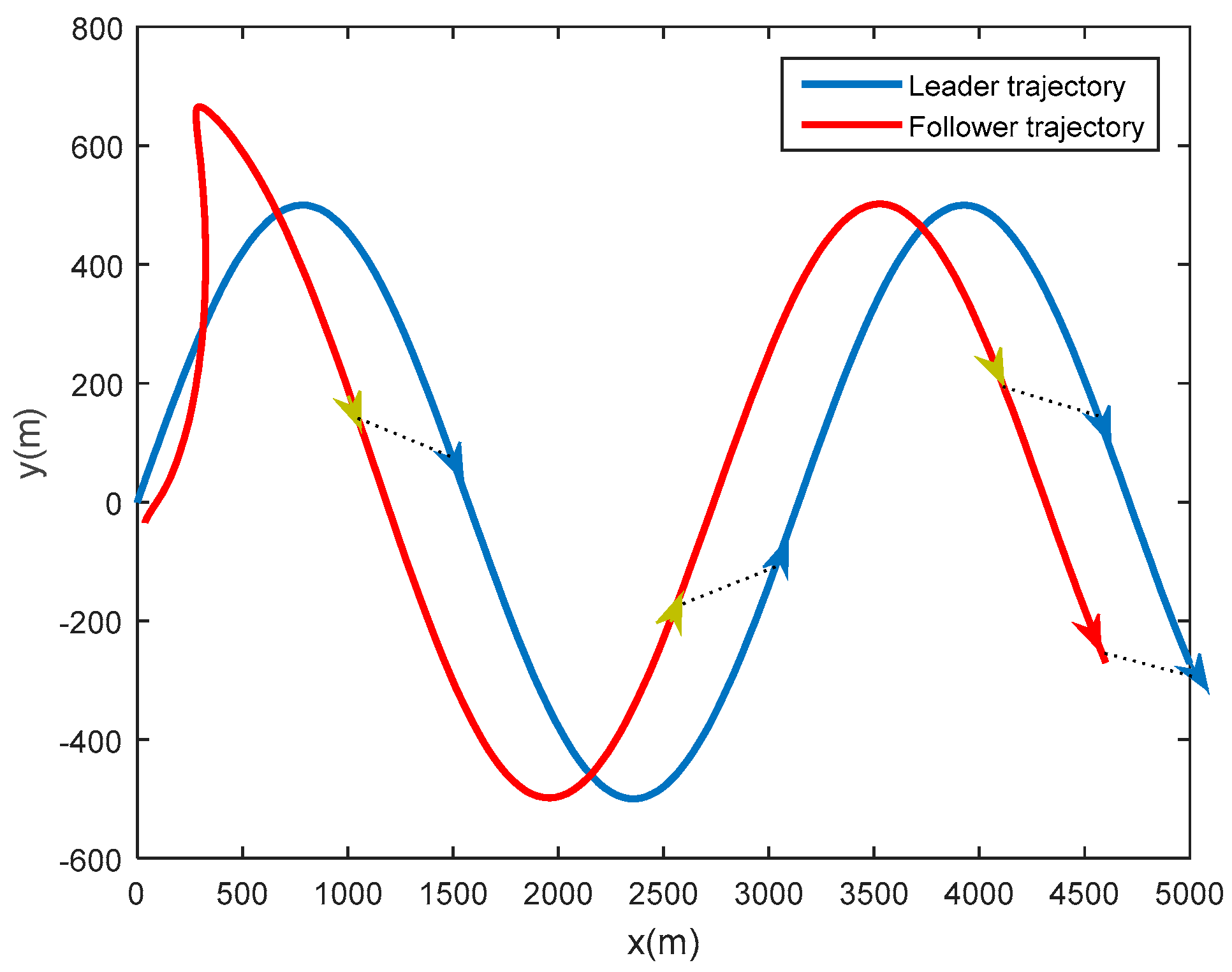
Figure 9 provides a visualization of the trajectories pursued by both robots. Notably, the leader robot’s trajectory is characterized by a sinusoidal pattern. Evidently, the follower robot adeptly tracks the leader robot’s path, successfully achieving the intended formation, as evident from the depicted trajectories in Figure 9.

By looking at Figure 6 and Figure 7, it can be found that, despite being in the presence of disturbance and uncertainty, the formation errors in Figure 6 become zero in less than 1 s, and this convergence does not have any overshoot, but the convergence of the upper bound of the uncertainties and disturbances to the constant bounded values in Figure 7 last about 20 s, and this convergence, of course, has no effect on maintaining the formation, which is also shown in Figure 9 as an example for the sinusoidal path of the leader.

4.3. Third Simulation Example

For the subsequent simulation, the focus shifts to the leader–obstacle formation paradigm, with the designated formation outlined as follows:

$$q_{des}={[l_{13}^d,l_{23}^d]}^T={[400,\hspace{1em}400]}^T$$

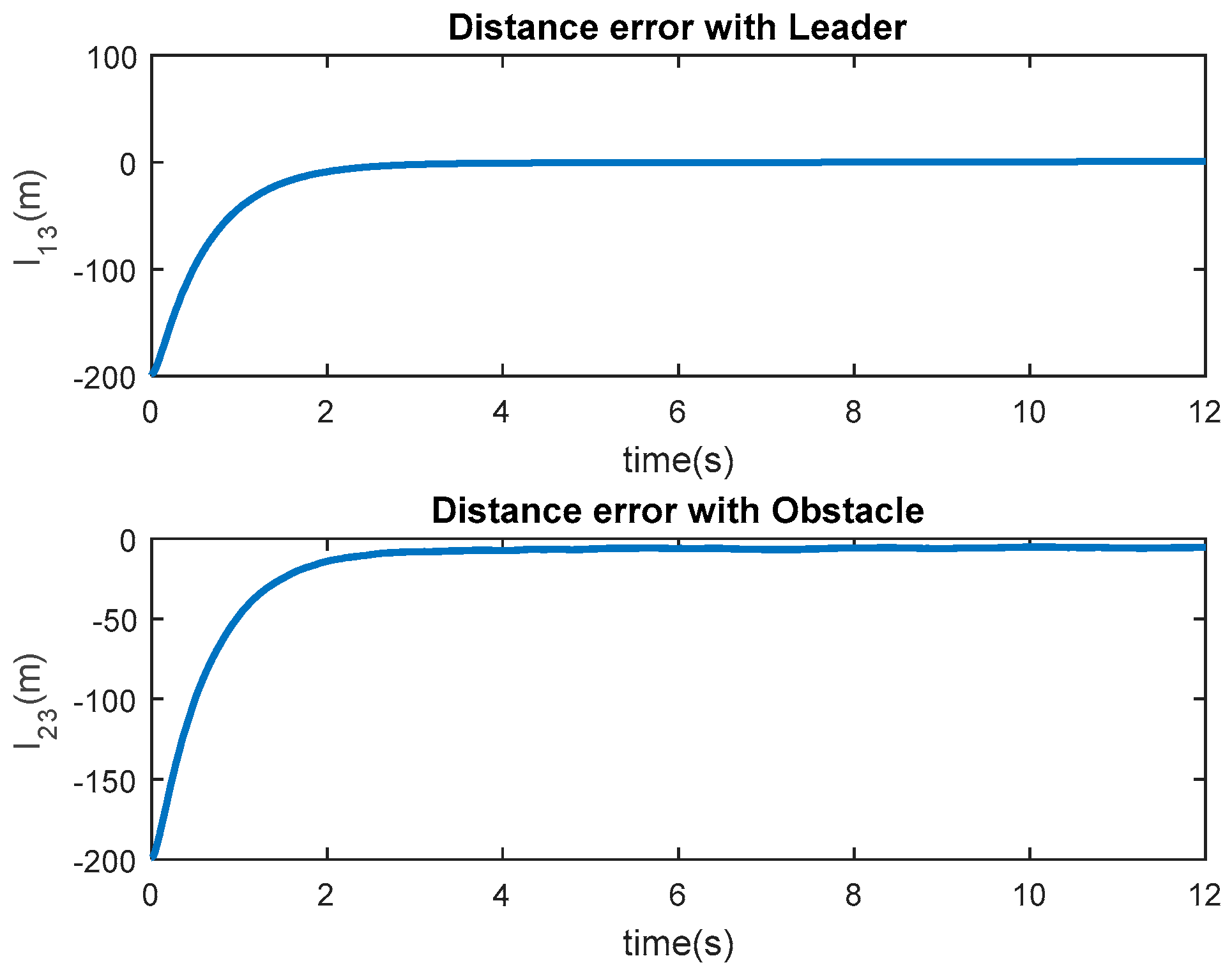
The control parameters are similar to the previous simulation. In this case, the formation errors are shown in Figure 10.

The distance error concerning the follower robot and the leader robot (first diagram in Figure 10) as well as the distance error involving the follower robot and the obstacle (second diagram in Figure 10) both exhibit a trajectory that converges toward zero. This convergence signifies that, as the obstacle draws near the leader–follower formation, the follower robot adeptly navigates around it, meticulously preserving a predefined separation from both the leader and the obstacle robots.

As we can see in this figure, the tracking error values between the follower robot and the leader robot, as well as the follower robot and the accelerated moving obstacle, both converge to zero in less than 4 s. The settling time is about 3.5 s and this convergence occurs without any overshoot. In addition, note that, similar to the previous simulation, here, the system is subject to additive uncertainties, and more importantly, the accelerations of both the leader and the obstacle are assumed as uncertainties in the system formation model and are unknown to the follower mobile robot.

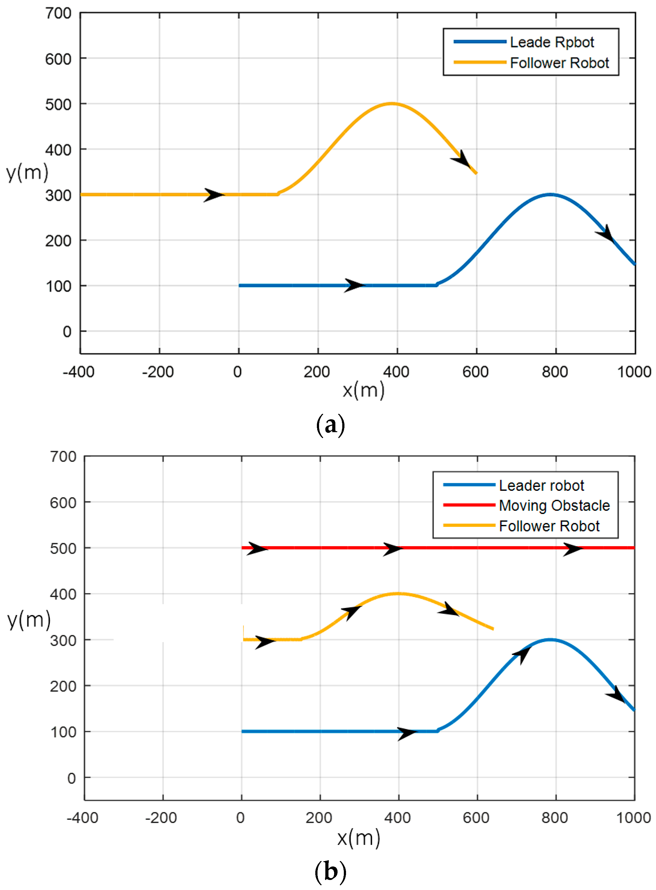
In Figure 11, the moving obstacle avoidance challenge is simulated. Considering the previous simulation parameters, in Figure 11a, the follower robot follows the leader robot with the desired formation. However, when an obstacle approaches the formation in Figure 11b, the follower robot changes his path to avoid it and to be at a safe distance from it, while keeping the desired formation with the leader as much as possible.

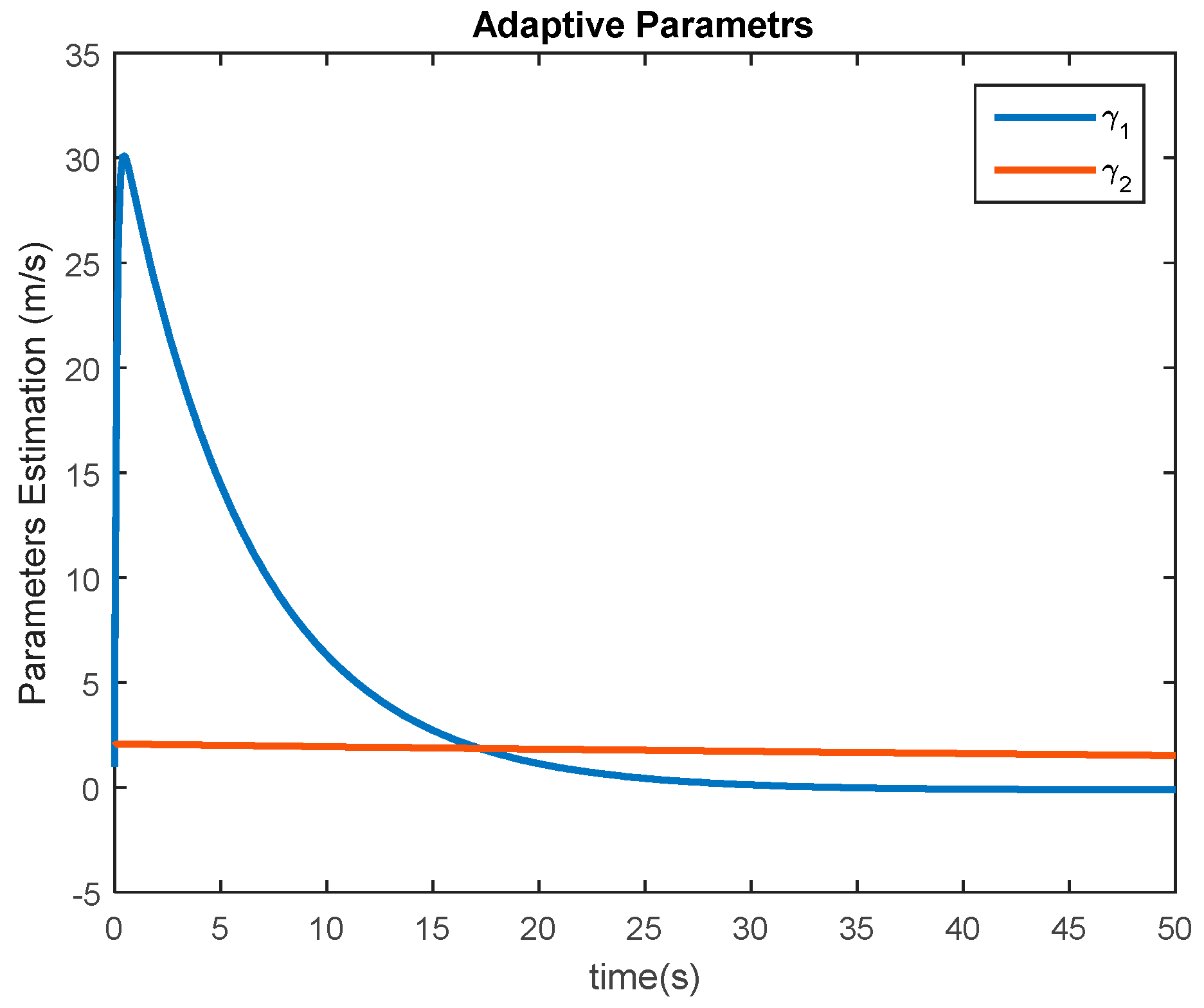
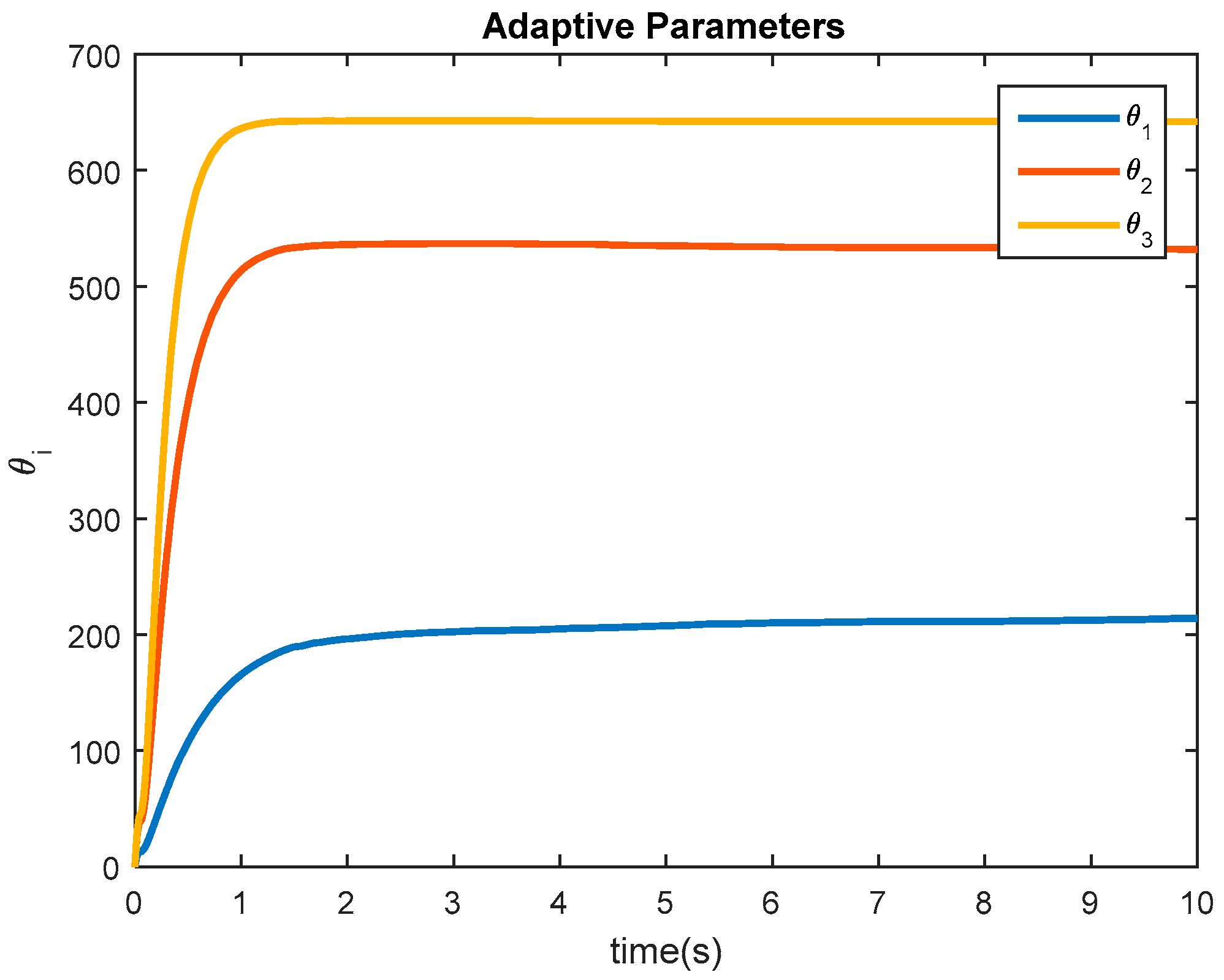
In Figure 12, the adaptive parameters of the control law (21–28), which are actually the outputs of the adaptive rule (28), are shown. These are the elements of vector ${\widehat{\theta }}_i,$ which is one of the parameters of the control law. As expected, and as we expect from stability proof of Theorem 1, the adaptive parameters in vector ${\widehat{\theta }}_i$ all have limited values and converge to constant values, which indicates the stability of the adaptive law.

5. Conclusions

In this paper, the problem of maintaining the leader–follower formation among mobile wheeled robots is dealt with. First, a robust adaptive control law is designed to deal with modeling uncertainties and unknown dynamics in the leader–follower formation model and according to the first-order kinematic model of formation. In this rule, the upper band of uncertainty is estimated using an adaptive rule. Next, in order to introduce acceleration in the formation model, a new robust adaptive control law was designed based on the second-order kinematic model, which establishes a formation despite disturbances, uncertainties, and unknown dynamics. In the designed controllers, the absolute velocity and acceleration of the leader robot, which are unknown for the follower, are considered as uncertainties, of which the upper bound is also unknown for the designer. In this paper, by considering the moving obstacle as a virtual leader, the problem of not encountering accelerated moving obstacles during formation, and considering uncertainty and disturbances, has also been solved.

References

- Zaidi, A.; Kazim, M.; Weng, R.; Wang, D.; Zhang, X. Distributed Observer-Based Leader Following Consensus Tracking Protocol for a Swarm of Drones. J. Intell. Robot. Syst. 2021, 101, 64. [Google Scholar] [CrossRef]
- Alfaro, A.; Morán, A. Leader-follower Formation Control of Nonholonomic Mobile Robots. In Proceedings of the 2020 IEEE ANDESCON, Quito, Ecuador, 13–16 October 2020; pp. 1–6. [Google Scholar]
- Wang, Z.; Wang, L.; Zhang, H.; Vlacic, L.; Chen, Q. Distributed Formation Control of Nonholonomic Wheeled Mobile Robots Subject to Longitudinal Slippage Constraints. IEEE Trans. Syst. Man Cybern. Syst. 2021, 51, 2992–3003. [Google Scholar] [CrossRef]
- Fallah, M.M.H.; Janabi-Sharifi, F.; Sajjadi, S.; Mehrandezh, M. A Visual Predictive Control Framework for Robust and Constrained Multi-Agent Formation Control. J. Intell. Robot. Syst. 2022, 105, 72. [Google Scholar] [CrossRef]
- Liang, X.; Wang, H.; Liu, Y.-H.; Chen, W.; Liu, T. Formation Control of Nonholonomic Mobile Robots without Position and Velocity Measurements. IEEE Trans. Robot. 2018, 34, 434–446. [Google Scholar] [CrossRef]
- Dai, S.L.; He, S.; Chen, X.; Jin, X. Adaptive Leader–follower Formation Control of Nonholonomic Mobile Robots with Prescribed Transient and Steady-state Performance. IEEE Trans. Ind. Inform. 2020, 16, 3662–3671. [Google Scholar] [CrossRef]
- Liu, Z.; Li, Y.; Wang, F.; Chen, Z. Reduced-Order Observer-Based Leader-Following Formation Control for Discrete-Time Linear Multi-Agent Systems. IEEE/CAA J. Autom. Sin. 2021, 8, 1715–1723. [Google Scholar] [CrossRef]
- Liu, X.; Ge, S.S.; Goh, C.-H. Vision-Based Leader–Follower Formation Control of Multiagents with Visibility Constraints. IEEE Trans. Control Syst. Technol. 2019, 27, 1326–1333. [Google Scholar] [CrossRef]
- Sanchez-Sanchez, A.G.; Hernandez-Martinez, E.G.; González-Sierra, J.; Ramírez-Neria, M.; Flores-Godoy, J.J.; Ferreira-Vazquez, E.D.; Fernandez-Anaya, G. Leader-Follower Power-based Formation Control Applied to Differential-drive Mobile Robots. J. Intell. Robot. Syst. 2023, 107, 6. [Google Scholar] [CrossRef]
- Maghenem, M.A.; Loría, A.; Panteley, E. Cascades-Based Leader–Follower Formation Tracking and Stabilization of Multiple Nonholonomic Vehicles. IEEE Trans. Autom. Control 2020, 65, 3639–3646. [Google Scholar] [CrossRef]
- Soorki, M.N.; Talebi, H.A.; Nikravesh, S.K.Y. A leader-following formation control of multiple mobile robots with active obstacle avoidance. In Proceedings of the 2011 19th Iranian Conference on Electrical Engineering, Tehran, Iran, 17–19 May 2011; pp. 1–6. [Google Scholar]
- Berkane, S.; Bisoffi, A.; Dimarogonas, D.V. Obstacle Avoidance via Hybrid Feedback. IEEE Trans. Autom. Control 2022, 67, 512–519. [Google Scholar] [CrossRef]
- Wu, J.; Luo, C.; Luo, Y.; Li, K. Distributed UAV Swarm Formation and Collision Avoidance Strategies Over Fixed and Switching Topologies. IEEE Trans. Cybern. 2022, 52, 10969–10979. [Google Scholar] [CrossRef]
- Duan, Y.; Yang, C.; Zhu, J.; Meng, Y.; Liu, X. Active obstacle avoidance method of autonomous vehicle based on improved artificial potential field. Int. J. Adv. Robot. Syst. 2022, 19, 17298806221115984. [Google Scholar] [CrossRef]
- Soorki, M.N.; Talebi, H.A.; Nikravesh, S.K.Y. A robust leader-obstacle formation control. In Proceedings of the 2011 IEEE International Conference on Control Applications (CCA), Denver, CO, USA, 28–30 September 2011; pp. 489–494. [Google Scholar]
- Dai, Y.; Kim, Y.; Wee, S.; Lee, D.; Lee, S. A switching formation strategy for obstacle avoidance of a multi-robot system based on robot priority model. ISA Trans. 2015, 56, 123–134. [Google Scholar] [CrossRef] [PubMed]
- Wang, W.; Huang, J.; Wen, C.; Fan, H. Distributed adaptive control for consensus tracking with application to formation control of nonholonomic mobile robots. Automatica 2014, 50, 1254–1263. [Google Scholar] [CrossRef]
- Ghommam, J.; Mahmoud, M.S.; Saad, M. Robust cooperative control for a group of mobile robots with quantized information exchange. J. Frankl. Inst. 2013, 350, 2291–2321. [Google Scholar] [CrossRef]
- Soorki, M.N.; Talebi, H.A.; Nikravesh, S.K.Y. A robust dynamic leader-follower formation control with active obstacle avoidance. In Proceedings of the 2013 IEEE International Conference on Systems, Man, and Cybernetics, Anchorage, AK, USA, 9–12 October 2011; pp. 1932–1937. [Google Scholar]
- Thuyen, N.A.; Thanh, P.N.N.; Anh, H.P.H. Adaptive finite-time leader-follower formation control for multiple AUVs regarding uncertain dynamics and disturbances. Ocean. Eng. 2023, 269, 113503. [Google Scholar] [CrossRef]
- Guillet, A.; Lenain, R.; Thuilot, B.; Martinet, P. Adaptable Robot Formation Control: Adaptive and Predictive Formation Control of Autonomous Vehiclesic. IEEE Robot. Autom. Mag. 2014, 21, 28–39. [Google Scholar] [CrossRef]
- Tang, X.; Yu, J.; Dong, X.; Li, Q.; Ren, Z. Distributed consensus tracking control of nonlinear multi-agent systems with dynamic output constraints and input saturation. J. Frankl. Inst. 2023, 360, 356–379. [Google Scholar] [CrossRef]
- Consolinia, L.; Morbidib, F.; Prattichizzo, D.; Tosques, M. Leader–follower formation control of nonholonomic mobile robots with input constraints. Automatica 2008, 44, 1343–1349. [Google Scholar] [CrossRef]
- Zhang, L.; Zhang, R.; Wu, T.; Weng, R.; Han, M.; Zhao, Y. Safe Reinforcement Learning with Stability Guarantee for Motion Planning of Autonomous Vehicles. IEEE Trans. Neural Netw. Learn. Syst. 2021, 32, 5435–5444. [Google Scholar] [CrossRef]
- Wu, T.; Zhu, Y.; Zhang, L.; Yang, J.; Ding, Y. Unified Terrestrial/Aerial Motion Planning for HyTAQs via NMPC. IEEE Robot. Autom. Lett. 2023, 8, 1085–1092. [Google Scholar] [CrossRef]
- Lagunas-Avila, J.; Castro-Linares, R.; Alvarez-Gallegos, J. Obstacle avoidance in leader-follower formation using artificial potential field algorithm. In Proceedings of the 2021 18th International Conference on Electrical Engineering, Computing Science and Automatic Control (CCE), Mexico City, Mexico, 10–12 November 2021; pp. 1–6. [Google Scholar]
- Arefanjazi, H.; Ataei, M.; Ekramian, M.; Montazeri, A. A robust distributed observer design for Lipschitz nonlinear systems with time-varying switching topology. J. Frankl. Inst. 2023, 360, 10728–10744. [Google Scholar] [CrossRef]
Disclaimer/Publisher’s Note: The statements, opinions and data contained in all publications are solely those of the individual author(s) and contributor(s) and not of MDPI and/or the editor(s). MDPI and/or the editor(s) disclaim responsibility for any injury to people or property resulting from any ideas, methods, instructions or products referred to in the content. |
© 2023 by the authors. Licensee MDPI, Basel, Switzerland. This article is an open access article distributed under the terms and conditions of the Creative Commons Attribution (CC BY) license (https://creativecommons.org/licenses/by/4.0/).