An Integrated Method for Reducing Arrival Interval by Optimizing Train Operation and Route Setting

Abstract

The arrival interval at high-speed railway stations is one of the key factors that restrict the improvement of the train following intervals. In the process of practical railway operation, sudden conflicts occur sometimes. Especially when the conflict arises at the station, because the home signal cannot be opened in time, the emergency may affect the adjustment of the train operation under the scheduled timetable, resulting in a longer train following interval or even delay. With the development of artificial intelligence and the deep integration of big data, the architecture of train operation control and dispatch integration is gradually improving from the theoretical point. Based on this and inspired by the Green Wave policy, we propose an integrated operation method that reduces the arrival interval by avoiding unnecessary stops in front of the home signal and increasing the running speed of trains through the throat area. It is a two-step optimization method combining both intelligent optimization and mathematical–theoretical analysis algorithms. In the first step, the recommended approaching speed and position are obtained by analytical calculation. In the second step, the speed profile from the current position to the position corresponding to the recommended approaching speed is optimized by intelligent optimization algorithms. Finally, the integrated method is verified through the analysis of two distinct case studies. The first case study utilizes data from the Beijing–Shanghai high-speed railway line, while the second one is based on the field test. The numerical result shows that the proposed method could save the entry running time effectively, compared with the normal strategy given by the train driver. The method can mitigate controllable conflict events occurring at the station and provides theoretical support for practical operation.

1. Introduction

In recent years, the high-speed railway has developed rapidly and become an important mode of transportation for people. However, under the influence of rain, storms, and other emergencies, track occupancy conflicts often occur when trains enter the station. The following train drivers are not aware of such conflicts in advance and are forced to stop, resulting in longer train following intervals and schedule instability [1]. This inevitably leads to significant delays. Thus, how to adjust the train operation strategy to compress the arrival interval in case of station conflicts is an urgent problem to be solved.

At the station, one of the main reasons for single train delays caused by disturbances is that the preceding train cannot complete the operation plan according to the scheduled timetable, resulting in the entering station conflict, which leads to the influence of the moving authority of the succeeding train [2]. The succeeding train has to stop before the home signal, awaiting clearance for entry. This leads to extended train arrival intervals and potential avoidable delays. Albrecht [3] proposed early the concept of proactively slowing down trains to prevent unplanned stops due to conflicts that could lead to delay events. However, this concept was limited by the automation capabilities of train scheduling at that time. Following this concept, Yun et al. further highlighted the methods for train control in such conflict scenarios but provided limited elaboration and application of the algorithms [4]. Moreover, researching train arrival route conflicts and applying the principle of approach unlocking at high-speed railway stations contributes to the compression of train arrival intervals. Diverse speed limits are employed across different railway segments and junctions to compress train arrival intervals and ensure safe distances between trains [5]. In addition, the management of real-time disruptions to the railway is often addressed by the real-time rescheduling of timetables to recover from a disrupted situation to a viable situation [6,7].

However, the optimization effect of these studies reaches a bottleneck in the existing system architecture. The current dispatching system and operation control belong to two levels of the system, which makes it difficult for dispatchers to control the running state of trains in the railway network in time. Meanwhile, drivers are also unable to obtain timely dispatch orders and are judged by their driving experience [8]. Specifically, in the event of an emergency, the dispatcher only has a macro understanding of part of the railway network. It is difficult for them to grasp the overall operation status of the system in real time, and they are often unable to communicate with drivers in time. At the same time, when the driver executes the dispatching command, he or she often judges the running condition based on driving experience, and the control effect on the train is not balanced.

With the improvement of the train scheduling automation capability, many research studies show that the collaborative optimization of train operation control and rescheduling allows rapid response to emergency events and enables further compression of train arrival intervals [9,10]. Under the integrated architecture, the dispatching system is able to accurately predict the train operating status and timetable, realizing real-time train scheduling and facilitating the quick response of the operation control system in planning the train trajectory [11]. Therefore, the time of the occupied train ahead to clear the platform is known based on the prediction of the train status of the real-time dispatching system. Based on the prediction of the opening time of the home signal, how to optimize the trajectory of the succeeding train to further compress the train arrival interval is the focus of our work. In order to quickly optimize the train trajectory within the restricted adjustment time, this paper adopts two popular types of computationally faster optimization algorithms to compute: one is meta-heuristic algorithms improved according to the habits of biological populations in nature [12,13,14], and the other is reinforcement learning (RL), which is developing rapidly in the field of artificial intelligence [15,16].

Based on the above mentioned, an integrated method of train operation and route setting is designed to reduce the train arrival interval. The method focuses more on the opening time of the home signal and the rapid optimization of the train trajectory. Moreover, the integrated method of reducing the arrival interval proposed in this paper is less restrictive for the station where the siding track is occupied, so it is generally feasible for entry conflict scenarios. The main contributions of this paper are as follows.

• We construct an integrated operation method to compress the arrival interval for the entry conflict scenario. This approach improves the passing speed by analyzing three entry strategies to avoid unnecessary stops in the throat area.
• The two-step method consists of mathematical analysis and optimization algorithms, with the former used to determine the entry operation strategy and the latter for calculating the optimal adjustment trajectory.
• The improved intelligent optimization algorithm can solve the recommended trajectory in a short period of time after obtaining the adjustment time. In addition, the validity and feasibility of the method are verified by simulation experiment and field test.

The main objective is to verify the feasibility of the integrated method through simulation and field test. The improved algorithms can realize the fast calculation of speed profiles and will potentially provide real-time adjustment of the trains. The remainder of this paper is organized as follows. Section 2 introduces the related work. The problem description is formulated by modeling the spacetime scenario in Section 3. In Section 4, we propose an integrated method of operation control and rescheduling for reducing the arrival interval. Section 5 gives two case studies to verify the method from different perspectives. Finally, conclusions are given in Section 6.

2. Related Work

In this section, we discuss the most relevant work on the ways to integrate real-time rescheduling solutions and the popular algorithms used for solving.

When there are no emergencies, the timetable can be executed according to the original plan. However, unexpected effects of weather and other factors are unavoidable during train operation. The time periods in the timetable are generally based on the processing time of each phase, such as headway time, dwell time and running time, plus extra buffer time [6]. Extended stage processing time due to emergency events often increases the train arrival interval and even causes train delays.

Therefore, a real-time rescheduling system is needed to be able to predict the future development of rail traffic accurately and to resolve potential route conflicts. D’Ariano et al. took into account the accurate monitoring of train positions and speeds, predicting in advance and resolving potential collision routes in real time [17,18]. The automated dispatching support system can provide effective assistance to dispatchers to effectively reduce delay propagation and minimize arrival delays at station and dispatch area boundaries. The system can be considered as part of a decision support system to assist dispatchers in controlling train traffic. Galapitage et al. developed a system that combines real-time driving recommendation calculations with real-time interchange rescheduling to reduce delays in the throat area [19]. The system detects a potential conflict 20 min before it occurs and calculates a new target time in the throat area to resolve the conflict. The connected driving advice system responds to the modified arrival time by calculating a new optimal speed profile. The delay prediction of the dispatching system [20] and the timely response of the operation control system to the train operation can further alleviate the serious consequences caused by the train delay.

To solve the problem of real-time train scheduling, the scholars improve the rapid response of the emergency not only from the system prediction perspective but also from the perspective of the model and method. The methods involved in train-rescheduling problems are divided into mathematical optimization, artificial intelligence, meta-heuristic algorithms and other methods generally. Each method has its inherent characteristics, advantages, and shortcomings in solving train-rescheduling problems.

The mathematical optimization algorithm is a kind of algorithm with a strictly theoretical basis. Some researchers establish mathematical optimization models for train-rescheduling problems, mostly integer linear programming (ILP) models, mixed-integer linear programming (MILP) models, and design optimization algorithms to solve the problem [21,22]. Wang et al. proposed two methods for solving the multi-train optimal control problem for different signaling systems, both of which are transformed into mixed-integer linear programming problems for solving [23]. And then, for the train-scheduling problem in which the subway line is completely blocked, Wang et al. considered multiple practical operational constraints and established a complex multi-objective mixed-integer linear programming model. To improve the solution accuracy, a two-stage method combined with a heuristic method is proposed to solve the problem [24]. Xu et al. developed a mixed-integer linear programming model to solve the rescheduling problem under micro-disturbances from a microscopic point of view, considering the train speed hierarchy in the quasi-moving block [25].

Since the model problem is strongly NP-hard, in practice, many scholars compute high-quality solutions in a shorter computation time with the help of intelligent optimization algorithms, such as meta-heuristic algorithms, as well as the RL algorithm.

The meta-heuristic algorithm is a way to overcome the weaknesses of pure mathematical planning for solving complex problems with nonlinearities. And it can simulate the characteristics of intelligent systems to design relevant computational methods [26,27]. The meta-heuristic algorithms are fast to compute and usually produce a feasible solution in a short time. Sama et al. combined meta-heuristic algorithms to solve the train-rescheduling problem, starting with a good initial solution of the fixed train route problem, obtained by a truncated branch and bound algorithm. Then a variable neighborhood search or label search algorithm was applied to improve the solution by relocating some sequences [28]. Krasemann used a greedy algorithm to generate better solutions in a short period of time as a way to reschedule due to railway emergencies [29]. For the delayed online rescheduling of high-speed trains, Yu et al. established a mathematical model and proposed a dynamic weighted particle swarm optimization algorithm to solve the problem [30]. But it does not further explain the effect of response measures and dynamic rescheduling time in emergencies.

Meta-heuristic algorithms and RL are both iterative optimization algorithms that are often used to solve problems, such as path planning and optimal control. Meta-heuristic algorithms use a defined objective function to guide the search process for a optimal solution, while RL utilizes the desired convergence approximation of the Markov chain process. It is a kind of learning strategy based on the principle of reward and punishment, which originates from the development and application of behavioral psychology [31]. The Q-learning algorithm is a typical model-free algorithm in RL. Semrov et al. proposed a train rescheduling method based on RL and applied the Q-learning principle. The principle consists of learning agents and their actions, environments, states, and rewards. Finally, the effectiveness of the Q-learning algorithm is evaluated in a real scenario [32]. In order to improve the efficiency of managing subway lines after disturbances, Su et al. researched the train-rescheduling problem and constructed a multi-objective optimization model. The paper divides the train operation process based on the classical spacetime network, and proposes a Q-learning-based solution approach to improve the solution efficiency [33].

These algorithms have a short computation time and often give a feasible solution in a short time, which is also the main reason why this paper adopts the above algorithms to solve the operation adjustment trajectory.

3. Problem Formulation

Considering the importance of the moment when the home signal allows trains to enter the station, in this paper, we use the terms open and close uniformly to emphasize the status of the home signal. In order to clearly describe the succeeding train operation adjustment problem caused by the entering station conflict, a three-dimensional problem model is constructed, and the normal operation scenario and the optimal operation scenario are replicated on a distance–time–speed spatial rectangular coordinate system as shown in Figure 1. In this section, Train 1 represents the preceding train, and Train 2 represents the succeeding train.

Static speed limit protection is shown as the red block area, with the red line representing the automatic train protection (ATP) profile at the moment of signal opening, which changes in real time depending on the opening time of the home signal. The two-dimensional plane of the speed–distance is shown in the grey area. The gold area represents the entry running time saved for optimization. According to Figure 1, the normal entering operation scenario and the optimal scenario are illustrated as follows.

3.1. Normal Operation Scenario

Due to an unplanned event, Train 1 could not complete the operation plan as scheduled resulting in conflict with Train 2 at the station. Train 2 is turned to brake when the home signal closes. At this moment, the initial condition is recorded as $(D_1,T_1,V_L)$. Train 2 reaches the home signal $(D_x,T_x,0)$ after the running time $T_r$. As the home signal closes, Train 2 stops in front of the home signal for the required waiting time $T_w$ to await dispatching instructions. When the home signal opens, Train 2 restarts and accelerates. Finally, it enters the station at the specified limit speed to stop at the side of station $(D_z,T_{t2},0)$.

The process of the succeeding train restarting at the home signal takes more time. In this case, the succeeding train may not be able to enter the station on time and even cause delays.

3.2. Optimal Operation Scenario

This paper only discusses two trains in this scenario to simplify the model. When the home signal opens, we consider the succeeding train not stopping and driving into the station at the recommended speed. This means that Train 2 reaches the adjustment point $(D_{opt},T_s,V_{opt})$ after a total adjustment time at the moment the home signal opens. The adjustment point of optimization is the recommended approach speed and the corresponding position. It is worth mentioning that in order to satisfy the optimization effect, the adjustment time should be greater than or equal to the sum of the braking and stopping time of the preceding train. This paper sets the adjustment time uniformly as $T_r+T_w$. Then the train runs by the best entry strategy and stops at the same position in the station $(D_z,T_{opt},0)$.

By comparing the train-running curves before and after optimization, the saving time for optimization can be observed in Figure 2. The blue and green lines are correspond to the normal and optimal trajectories of the succeeding train, while the black line indicates the trajectory of the preceding train. The external operating conditions and internal disturbance factors affecting the train operation are complex and difficult to model accurately. Thus, the method in this paper treats Train 1 and Train 2 as independent single mass point models. The predicted opening time of the home signal is used as the bridge between the two models. The succeeding train is adjusted for operation optimization based on the opening time of the home signal to save the entry running time.

4. An Integrated Operation Method for Reducing Arrival Interval of Trains

The process of optimizing the operation control considering the opening time of the home signal is divided into two stages as shown in Figure 3. Firstly, the adjustment point is obtained by the analysis of the entry operation strategy. And then the train trajectory before the adjustment point is designed by using the meta-heuristic algorithm.

4.1. Analysis of the Entry Operation Strategy

In the first step, we use numerical analysis to find the optimal adjustment point in stage II. To facilitate the theoretical analysis of the entry station pattern in this section, a two-dimensional speed–distance entry operation scenario is drawn based on Figure 1, and a right-angle coordinate system is established, with the horizontal axis representing the distance and the vertical axis representing the current speed of the train. Thus, the coordinate points indicate the train location and speed status. Furthermore, the ATP is the updated speed limit protection curve after the home signal opens.

According to Pontryagin’s maximum principle, the optimal operating curve is composed of four conditions: maximum acceleration, cruise, maximum braking and coasting. As the model mainly focuses on the succeeding train caused by the entry conflict, the coasting condition is not considered [34]. The optimized entry trajectory can be planned only after the home signal opens and the ATP limit is updated, so either operation condition can be selected from the adjustment point. Combined with the entry station scenarios described in the previous section, three entry operation strategies can be inferred, which are maximum acceleration–cruise–maximum braking (MA-CR-MB), maximum acceleration–maximum braking (MA-MB), and maximum acceleration (MA). The initial point $(x_b,v_b)$ that allows the most time saved is on the normal speed profile. The parameters are described uniformly in

Table 1. Parameter description.

Items	Symbol	Unit
Position of signal	$x_x$	m
Position of entry station	$x_j$	m
Length of line	$x_z$	m
The current location	$x_b$	m
The current speed	$v_b$	m/s
Station speed limit	$v_z$	m/s
Line speed limit	$v_L$	m/s
Speed of intersection point in MA-MB	$v_j$	m/s
Train traction acceleration	$a_t$	m/s${}^2$
Train braking deceleration	$a_b$	m/s${}^2$
Entry running time of Pattern i	$T_i$ (i = 1, 2, 3)	s
Time saved of Pattern i	$\Delta T_i$ (i = 1, 2, 3)	s
Original entry running time	$T_o$ (i = 1, 2, 3)	s

All parameters used in this paper are in absolute values except $\Delta T_i$.

.

The theoretical analysis of the method is based on the following assumptions:

• The acceleration and deceleration process is an ideal uniform variable speed process.
• The endpoint of the planned entry running curve is at position $(x_z,0)$ in Figure 4.
• The platform length allows the train to reach the speed limit in the throat area and cruise in either pattern.
• To simplify the train speed profile optimization model, there are no other temporary speed limits between stations, and the line speed limit is uniformly $v_L$.
• The introduction of the strategy of an operation mainly ignores the interlocking mechanism in the throat area, assuming that the receiving path is locked and released as a single entity.

According to Table 1, $T_o$ is the time for the original entry running before optimization:

$$T_o=\frac{x_z-x_x-\frac{v_z^2}{2a_t}-\frac{v_z^2}{2a_b}}{v_z}+\frac{v_z}{a_b}+\frac{v_z}{a_t}$$

(1)

The train entry running time saved by each entry operation pattern $\Delta T_i=T_i-T_o$ (i = 1, 2, 3), so $\Delta T_i$ is negative. It is important to note that each entry operation pattern has a different range of initial speed depending on the operating conditions.

4.1.1. Pattern of MA-CR-MB

The entry operation pattern contains three conditions of acceleration, cruise and braking as shown in curve ➀ in Figure 4.

The initial state $(x_b,v_b)$ is far from the station. The train receives information about the open timing of the home signal ahead, accelerates to the static speed limit of the line $v_L$ first, and then cruises at the static speed limit. When the speed reaches the ATP profile, the working condition is switched to maximum braking and the train decelerates to the state $(x_j,v_z)$ for entering the station.

The equation for the time saved $\Delta T_1$ as a function of $v_b$ is as follows:

$$\Delta T_1=\left(\frac{1}{2a_b\times v_L}-\frac{1}{2a_t\times v_L}\right)\times {v_b}^2-\frac{v_b}{a_t}+\left(\frac{v_L-2v_z}{2a_t}+\frac{x_j-x_x}{v_L}+\frac{v_L-v_z}{a_b}+\frac{x_x-x_j+\frac{v_z^2}{2a_t}}{v_z}\right)$$

(2)

4.1.2. Pattern of MA-MB

The entry operation pattern contains two conditions of acceleration and braking, as shown in curve ➁ in Figure 4. The pattern is special for solving, which has an intersection with a switching mode.

The initial state $(x_b,v_b)$ is at a moderate distance from the platform. The train is given permission to enter the station, accelerates to the static speed limit first, switches the working condition to the maximum brake, and then the train decelerates to the state $(x_j,v_z)$ into the station.

The equation for the time saved $\Delta T_2$ as a function of $v_b$ is as follows:

$$\Delta T_2=\left\{\frac{1}{a_t}(v_j-v_b)\right.\left.+\frac{v_j}{a_b}\right\}-\frac{v_z}{a_t}-\frac{v_z}{a_b}+\frac{x_x-x_j+\frac{v_z^2}{2a_t}}{v_z}$$

(3)

where $v_j$ is represented by the line parameter constants as follows:

$$v_j=\sqrt{\frac{2a_t\times a_b\times (x_j-x_x)+v_z^2\times a_t}{a_t+a_b}+{v_b}^2}$$

(4)

4.1.3. Pattern of MA

The entry operation pattern includes only the acceleration condition as shown in curve ➂ in Figure 4.

The pattern is more special, as the length of the throat area has to satisfy the condition $(x_j-x_x)\le v_z^2\times 2a_t$; otherwise, the train traction acceleration in the MA pattern will be adjusted to be less than the maximum traction.

The equation for the time saved $\Delta T_3$ as a function of $v_b$ is as follows:

$$\Delta T_3=\left(\frac{\frac{1}{2a_t}+\frac{1}{2a_b}}{v_z}\right)\times v_b^2-\frac{v_b}{a_t}$$

(5)

Based on the above calculation, it is found that $\Delta T_i$ (i = 1, 2, 3) is a quadratic function of $v_b$ in three patterns. That means if the entry operation condition includes the applicable entry length and speed limit, the quadratic equation can be solved, and the adjustment point in the best entry strategy can be calculated.

4.2. Analysis of the Optimal Adjustment Trajectory

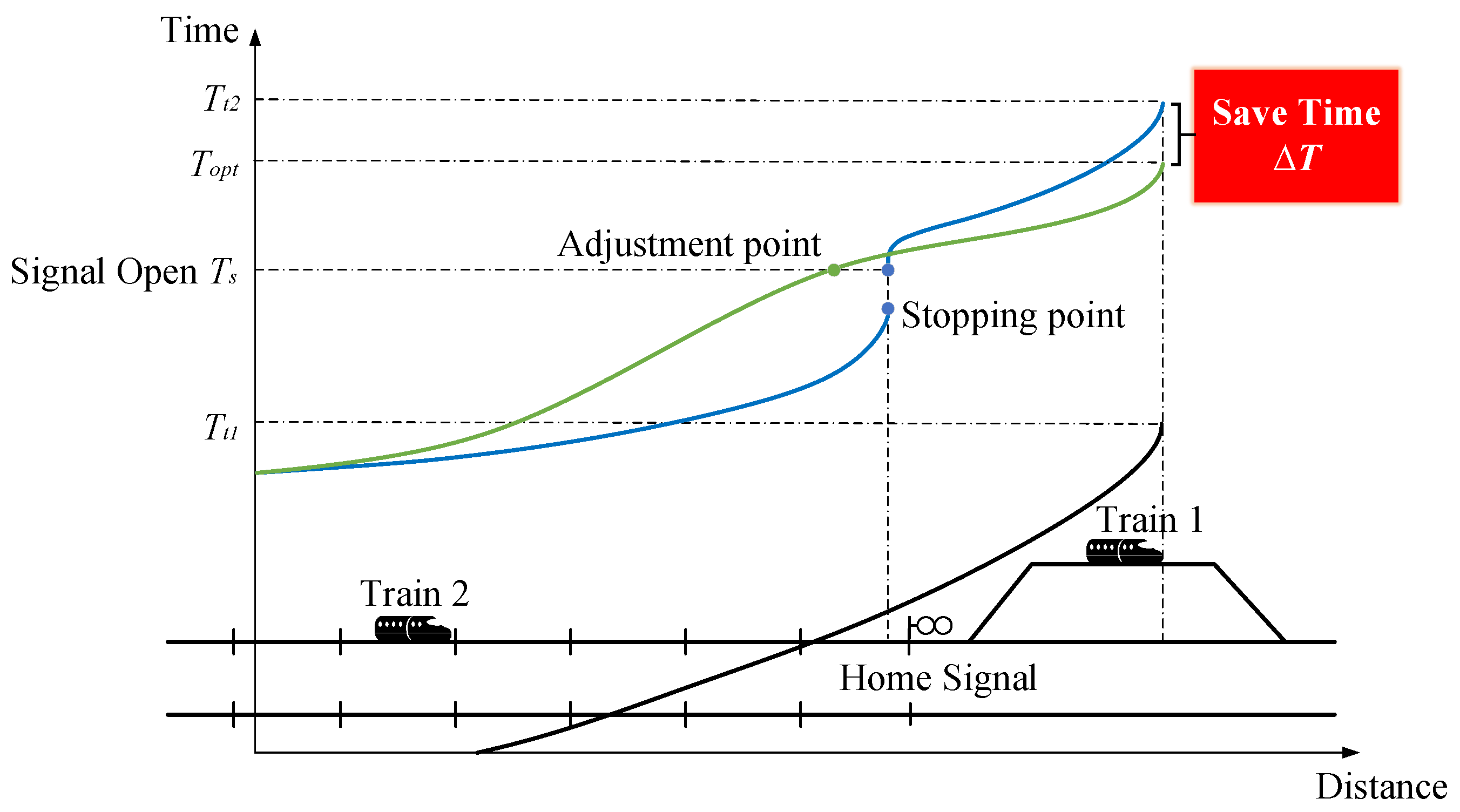
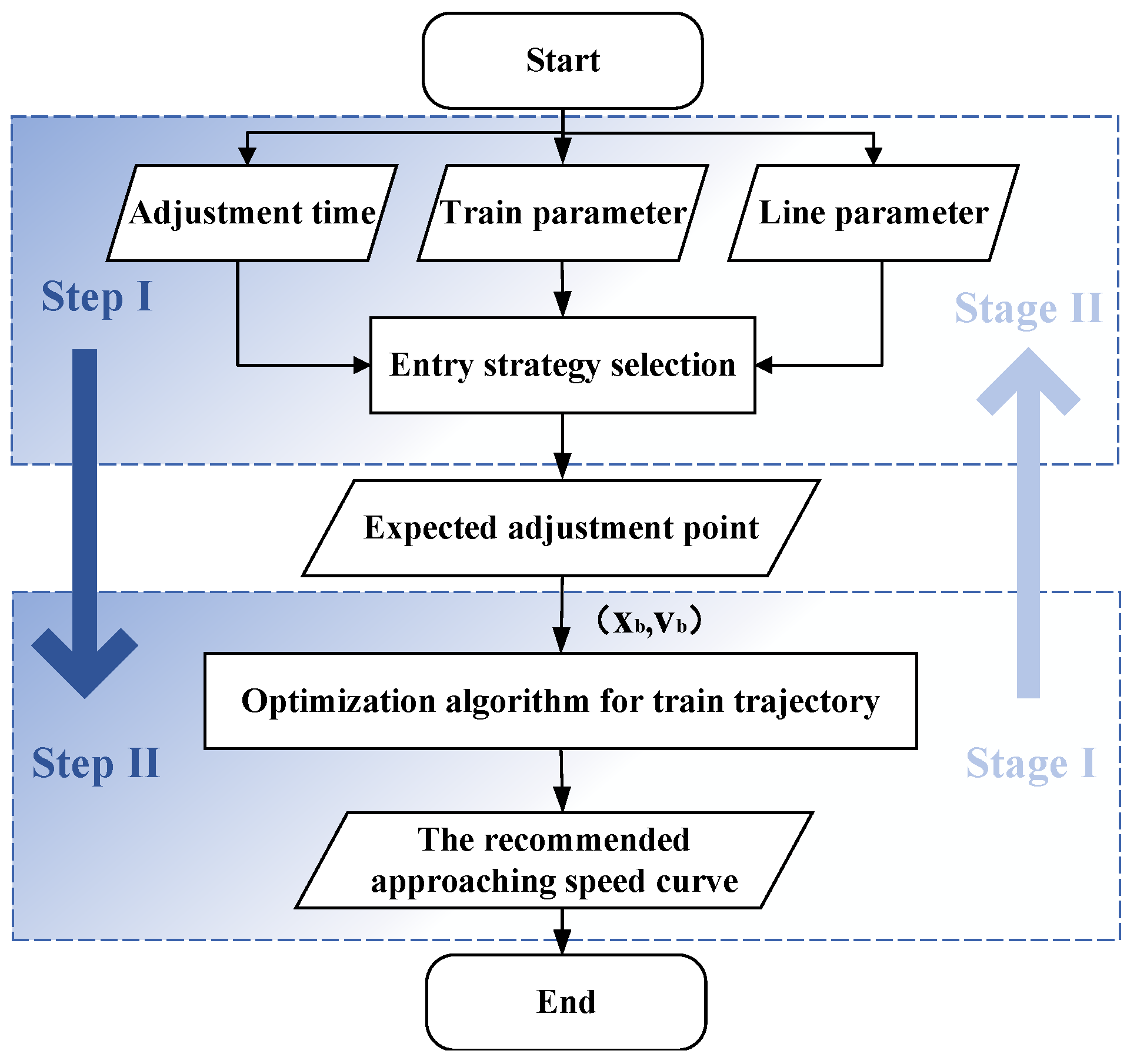
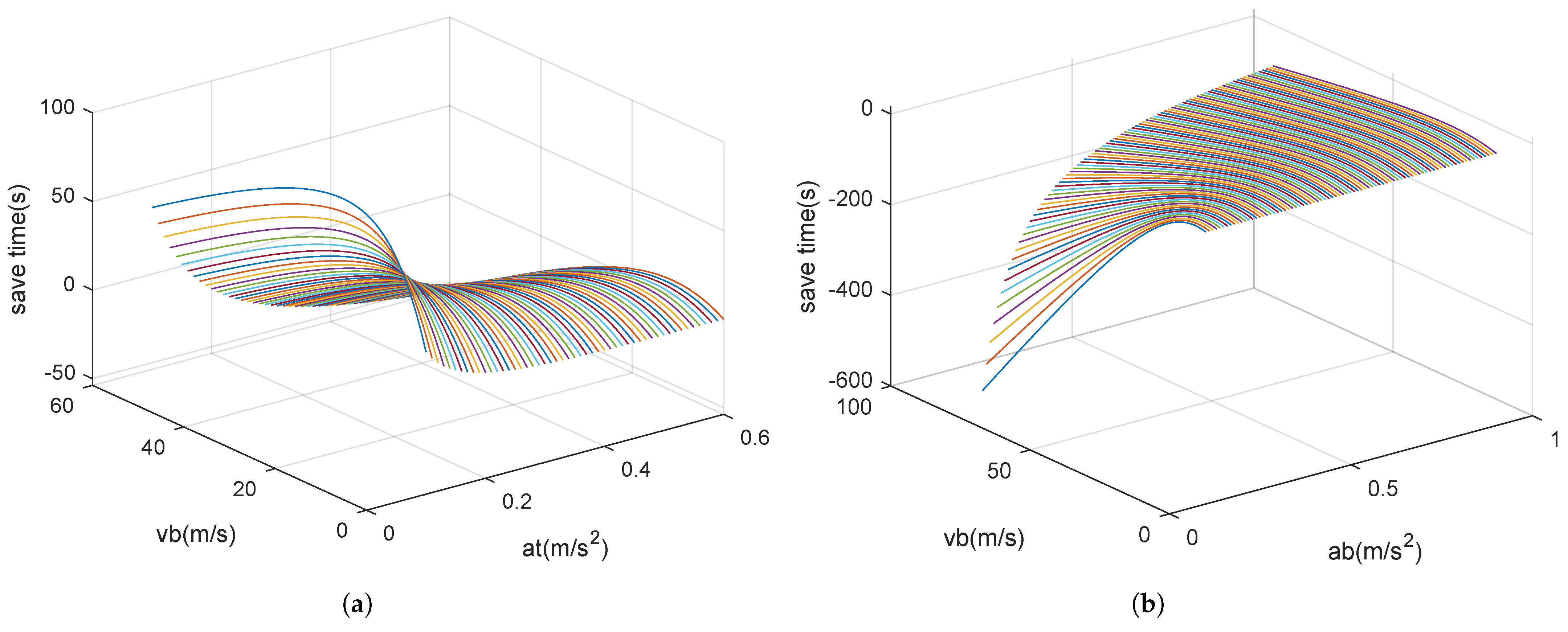
In the next step, we apply the meta-heuristic algorithm and Q-learning algorithm to solve the optimal adjustment trajectory based on the strategy calculation in the first step at the stage I. The train operation trajectory is the movement from the initial state to the target state after a certain running time, where the running time is predicted by the train dispatching system. Specifically, the optimal trajectory should satisfy the condition that the train reaches the adjustment point $(x_b,v_b)$ in time, during the total adjustment time $T_r+T_w$, at which time the home signal opens.

4.2.1. The Improved Meta-Heuristic Algorithm

The meta-heuristic algorithm is one of the important directions in the development of artificial intelligence today, and it embodies characteristics that are different from the traditional intelligent optimization algorithms of the past [35]. The algorithm is a valuable optimization strategy that solves complex optimization problems by simulating the search behavior of nature with a core of swarm intelligence algorithms. It contains a variety of algorithms, such as classical particle swarm optimization (PSO) and the genetic algorithm (GA). In recent years, a variety of new algorithms have emerged, such as grey wolf optimizer (GWO). In this section, the classic PSO algorithm of heuristic algorithms and the popular GWO algorithm are used to solve the problem.

(1)

PSO Algorithm

The basic principle of the particle swarm algorithm can be summarized by a flock of birds allowing other birds to discover the location of the food source by passing information about their own location to each other throughout the search process. The other birds constantly update their flying speed and direction, and eventually the whole flock can gather around the food source, that is, the optimal solution has been found.

Each particle continuously updates its position and speed through the fitness value determined by the objective function to find the optimal solution of the problem. The objective function set by the algorithm is an error function. The closer the particle is to the target state point, the smaller the value of the objective function. That is consistent with how birds forage for food.

Assuming that the dimension of the search space is d and the coordinates of each particle are $X_i=(x_{i1},x_{i2},...,x_{id})$, the speed of flight of each particle is $V_i=(v_{i1},v_{i2},...,v_{id})$. For the first i particles, the best historical position through which it passes is denoted as $pbes{t}_i=(p_{i1},p_{i2},...,p_{id})$. The best position of all particles found so far in the whole population is noted as $gbes{t}_i=(g_{i1},g_{i2},...,g_{id})$. The particle constantly updates its speed and position according to the changes in these two best positions:

$$\begin{array}{c}\hfill v_{ij}(k+1)=w{v}_{ij}\left(k\right)+r_1{c}_1(p_{ij}-x_{ij}\left(k\right))+r_2{c}_2(g_{ij}-x_{ij}\left(k\right))\end{array}$$

(6)

$$x_{ij}(k+1)=x_{ij}+v_{ij}(k+1)$$

(7)

where w (w > 0), $c_1$ and $c_2$ are the learning factors, and $r_1$ and $r_2$ are random numbers between [0, 1]. Usually the range of the position change is limited to [$X_{min xd},X_{max xd}$], and the range of speed change is limited to [$V_{min xd},V_{max xd}$]:

(2)

GWO Algorithm

The grey wolf optimizer algorithm was proposed by Mirjalili et al. based on the cooperative predatory behavior of grey wolf packs [36]. The leader of the wolf pack is at the top of the population pyramid. The $\alpha$ has the highest decision-making power and is responsible for matters in the pack, such as hunting and roosting. The second layer is the intelligent group $\beta$ of the wolf group, which mainly assists the $\alpha$ in making decisions and conveying instructions downward. The $\beta$ will take over the position of $\alpha$ if the leader position is missing. The third layer $\delta$ wolves obey the leadership of $\beta$ and $\alpha$ wolves and are mainly responsible for such matters as sentry watching and scouting. The bottom layer of the pyramid is $\omega$ wolves, who obey the leadership of the superior and are mainly responsible for the balance of the internal relationship of the middle group. Each grey wolf represents a potential solution, and the objective function value indicates the degree of merit of each solution. During the iteration of the algorithm, the goal is to gradually bring the grey wolf population closer to the global optimal solution, which means that the objective function value gradually decreases. The grey wolves with lower objective function values are considered to be closer to the solution of the optimization problem, and thus they play a role similar to that of prey in the grey wolf population, a target for other grey wolves to find.

The hunting behavior of the grey wolf population is mainly divided into three steps:

• Tracking, chasing and approaching the prey;
• Chasing and encircling the prey and harassing until it stops moving;
• Attacking the prey.

After the leader of the wolves $\alpha$ determines the location of the target prey, it will give the command for the wolf to surround the prey and update the location of the search in each iteration of the calculation, defining the behavior of the wolf pack in surrounding the prey by the succeeding equation:

$$\overrightarrow{D}=|\overrightarrow{C}·\overrightarrow{X_p}\left(t\right)-\overrightarrow{X}\left(t\right)|$$

(8)

$$\overrightarrow{X}(t+1)=\overrightarrow{X_p}\left(t\right)-\overrightarrow{A}·\overrightarrow{D}$$

(9)

where $\overrightarrow{D}$ is the distance between individual wolves and their prey, and t represents number of algorithm iterations. $\overrightarrow{X_p}\left(t\right)$ is the position vector of the prey in t iterations. $\overrightarrow{X}\left(t\right)$ is the position vector of the wolf in t iterations. $\overrightarrow{A}$, $\overrightarrow{C}$ are coefficient vectors expressed by the succeeding equation:

$$\overrightarrow{A}=2\overrightarrow{a}·\overrightarrow{r_1}-\overrightarrow{a}$$

(10)

$$\overrightarrow{C}=2\overrightarrow{r_2}$$

(11)

where $\overrightarrow{a}$ is convergence factor that decreases linearly from 2 to 0 with the number of iterations. $r_1$ and $r_2$ are random numbers between [0, 1].  With the help of the coefficient vector $|\overrightarrow{A}|> 1$ indicating that the wolves explore outward and $|\overrightarrow{A}|<1$ indicating that the wolves explore inward and converge toward the prey, the convergence factor $\overrightarrow{a}$ ensures convergence to the optimal value in the global search.

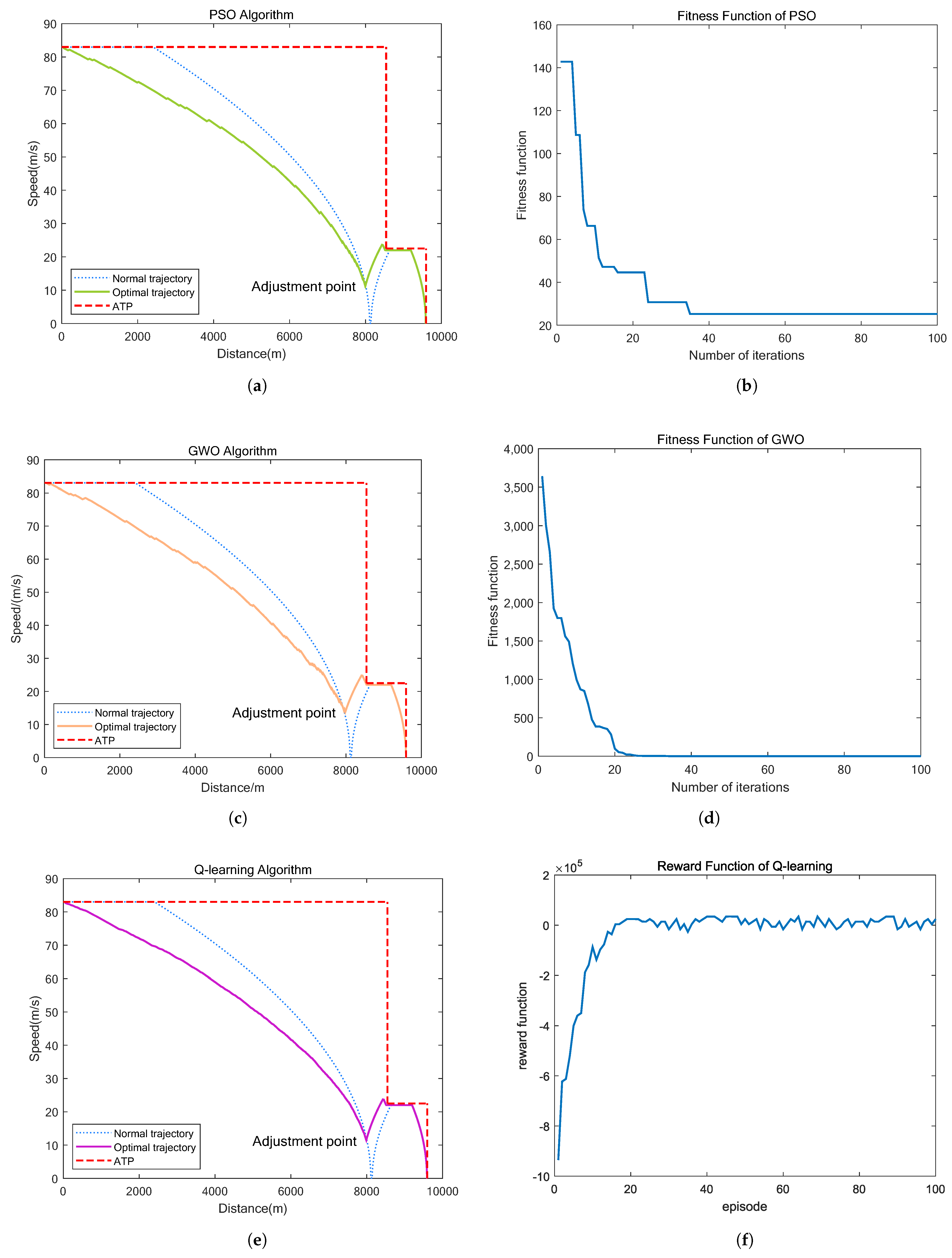
The standard GWO and PSO algorithms have position updates in the continuous domain, which are only suitable for solving continuous optimization problems and cannot directly solve problems in the discrete domain. Therefore, we improve the metaheuristic algorithm by using a coding transformation method that converts continuous spaces to discrete spaces and real numbers to integers based on the idea of mathematical mapping. The whole train operation process is discretized, and the algorithm searches in the discretized space for feasible solutions and converges to the optimal solution. After each iteration is completed, an integer conversion of the condition sequence code is required. Assuming that the train operation curve optimization process contains N discrete substage, the condition code corresponding to each discrete substage process is $N_i\in [0,6]$. Each substage corresponds to a different rate of speed change, which is $a_n$.

The fitness function of the improved meta-heuristic algorithm (Algorithm 1) is calculated for each particle or grey wolf during each iteration. In the iterative process of the algorithm, the optimal fitness is obtained by comparison. The goal is to keep approaching the target optimal adjustment point:

$$F=|\sum _{i=1}^n{x}_i-x_b|+|v_L+\sum _{i=1}^n{a}_i\times \Delta t-v_b|$$

(12)

Algorithm 1 The improved meta-heuristic algorithms

Input:  $N_{iter}$: The maximum iteration; M: The population quantity; $\Delta t$: Train control circle; $T_r+T_w$: The total adjustment time; $(x_b,v_b)$: The target state Output:  The near optimal working condition solution; The fitness function; 1:  Calculate the substage numbers N, $N=(T_r+T_w)/\Delta t$ 2:  Initialize the population $X={\left(x_{ij}\right)}_{N\times M}, 0\le x_{ij}\le 6$ and algorithm parameters 3:  while $k\le N_{iter}$ do 4:     while $m\le M$ do 5:        Update the position of $X_i$ by fitness 6:        Operated by the heuristic algorithm structure 7:        $m=m+1$ 8:     end while 9:     Calculate the fitness F by (12) 10:    Record the fitness of each optimal state 11:    $k=k+1$ 12: end while

4.2.2. The Improved Q-Learning Algorithm (Algorithm 2)

Q-learning is a classic value-based reinforcement learning algorithm, and the Q value represents the expected cumulative reward in a given state and action:

$$Q:S\times A\to \mathbb{R}$$

(13)

where S denotes the state space explored by Q-learning and A is the action space. The reward is an evaluation of the changes in the state of the environment caused by the action taken, which is an important guidance for the training process. It is divided into active reward and negative reward, and the merit of the reward function design directly determines the effect of reinforcement learning. The reward function is shown in (14), in which r is a set reward constant:

$$Q\left(s_{t+1}\right|s_t,a_t)\left\{\begin{array}{c}10\ast r,\mathrm{if}{a}_t\mathrm{is}\mathrm{active}\mathrm{action}\hfill \\ r,else\hfill \\ -10\ast r,\mathrm{if}{a}_t\mathrm{is}\mathrm{negative}\mathrm{action}\hfill \end{array}\right.$$

(14)

The algorithm is initialized with an initial value Q of 0. At the moment of t, the state of the environment is defined as $s_t$, the intelligent agent selects an action $a_t$, and receives the reward $r_t$. Specifically, the deviation from the target state is calculated for the current state during training, and the action is decided to be positive or negative based on the size of the error. And then, the environment changes its state to a new state $s_{t+1}$ as the result of the agent’s action. The main idea of the algorithm is to construct a Q-table of states and actions to store the Q-values, and then based on the Q-values to select the action that can obtain the maximum benefit. The specific form of Bellman’s equation used to update the Q-values is as follows:

$$Q^{new}(s_t,a_t)\leftarrow (1-\alpha )·Q(s_t,a_t)+\alpha ·(r_t+\gamma ·\underset{a}{max}Q(s_{t+1},a))$$

(15)

where $r_t$ denotes the reward value obtained from state $s_t$ to state $s_{t+1}$. $\alpha$ is the learning factor ($0<\alpha \le 1$), which defines the weight that an old Q-value will learn from a new Q-value, with a value of 0 meaning that the agent will not learn anything (the old information is important), and a value of 1 meaning that the newly discovered information is the only information that matters. $\gamma$ is the discount factor ($0\le \gamma \le 1$), which defines the importance of future rewards. A value of 0 means that only short-term rewards are considered, where a value of 1 gives more importance to long-term rewards.

The Q-table built by the algorithm is discrete and contains only a limited number of states and actions, corresponding to the way that the train state space discretized in the previous section. Each row in the Q-table represents the state of the train’s operating position, and each column represents the value of the working condition taken. We refer to each exploration of the agent as an episode. In each episode, an episode ends when the agent reaches the target state from the initial state, and then proceeds to another episode. In order to avoid the exploration process falling into a locally optimal solution, a dynamic $\epsilon -greedy$ optimization strategy is used for exploration during the training process. When the train position is at $s_t$, the action is randomly selected with probability of $\epsilon$, that is, the operating condition is shown in

Table 2. Working condition coding.

Coding of ${\mathit{N}}_{\mathit{i}}$	Working Condition
0	100% Braking
1	80% Braking
2	60% Braking
3	100% Tracking
4	80% Tracking
5	60% Tracking
6	Cruising

. And the action corresponding to the maximum value in row $s_t$ of states in Q-table is selected with probability $1-\epsilon$. Initially, a larger $\epsilon$ is used to achieve higher exploration efficiency, and the epsilon decay factor is set to reduce the value of $\epsilon$ with state migration.

Algorithm 2 The improved Q-learning algorithm

Input:  $\alpha$: The learning factor; $\gamma$: the discount factor; $\epsilon$: The initial epsilon; epsilon decay factor; episode maximum; the Q-table size; $\Delta t$: Train control circle; $T_r+T_w$: The total adjustment time; $(x_b,v_b)$: The target state Output:  The near optimal working condition solution; The reward function; 1:  for Episode = 1, 2, … do 2:     Initialize the initial state 3:     Dynamically update $\epsilon$ using epsilon decay factor 4:     repeat 5:        $a_t$ is selected based on Q-table using $\epsilon -greedy$ strategy 6:        Perform $a_t$, observe the reward $r_t$ by (14) and the next state $s_{t+1}$ 7:        Update Q-table by (15) 8:        $s_t\leftarrow s_{t+1}$ 9:        reward = reward + $r_t$; 10:    until $s_t$ reaches the terminal state 11:    Record the reward of each episode 12: end for

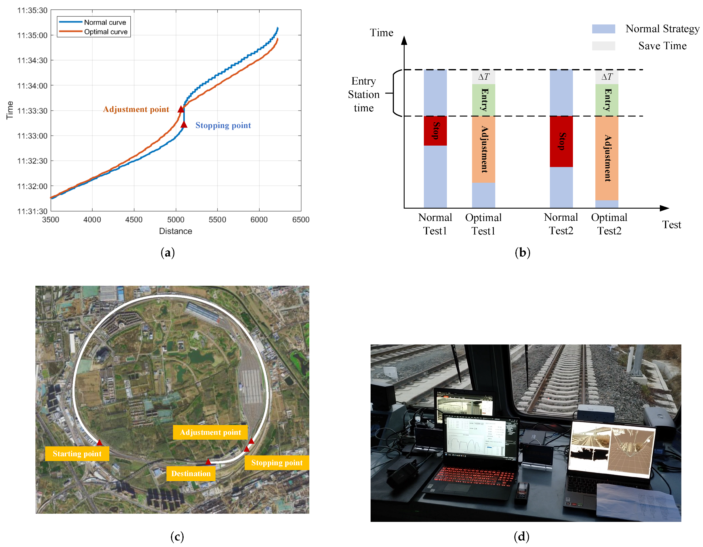
5. Experimental Results

Two case studies are presented in this section. The first case validates the integrated operation method for reducing the arrival interval. The data are selected from a typical high-speed railway station on the Beijing–Shanghai line. The second case verifies the method on a field test and proves that the stopping time does not affect the saving time. The results show that the optimal strategy could save the entry running time by 10–30%, compared with the normal strategy given by driver. When the entry station conflict causes delay, reducing the entry running time can greatly alleviate delay. The proposed method is implemented in MatlabR2021a on a computer with an Intel Core i7–8700 CPU @ 3.20 Ghz and 16 GB RAM running Windows 10 x64 Edition. It is assumed that the preceding train leaves the station platform and the home signal opens within the same time error in the simulation line.

5.1. Case Study 1: The Train Speed Profile Optimization Model Based with Simulation Line for Succeeding Train

The verification of the three entry operation strategies using the analysis algorithm relies on MatlabR2021a, which requires setting the line parameters as known quantities of input, and the output is the saving time for the entry operation strategy. With reference to the general railway line in the Beijing–Shanghai line, we set a simulation scenario. The parameters used in the simulation are described in

Table 3. The Main Parameters of Simulation.

Category	Items	Symbol	Value	Unit
Line parameters	Station speed limit	$v_z$	22	m/s
	Line speed limit	$v_L$	83	m/s
	Train traction acceleration	$a_t$	0.5	m/s${}^2$
	Train braking deceleration	$a_b$	0.6	m/s${}^2$
	Length of line	$x_z$	9594	m
	Length of throat area	$x_j-x_x$	400	m
	Length of station	$x_z-x_x$	1450	m
	Initial train position	$x_0$	0	m
	The adjustment time	$T_r+T_w$	170	s
PSO	The population quantity	$M_{pso}$	40	/
	The maximum iteration	$N_{iter\left(pso\right)}$	100	/
	The inertia weight of PSO	w	0.5	/
	The learning factors of PSO	$c_1,c_2$	0.4	/
GWO	The population quantity	$M_{pso}$	40	/
	The maximum iteration	$N_{iter\left(gwo\right)}$	100	/
Q-learning	The learning factor	$\alpha$	0.2	/
	The discount factor	$\gamma$	0.9	/
	The initial epsilon	$\epsilon$	1	/
	The epsilon decay factor	$\epsilon$$-decay$	0.82	/
	The episode maximum	$episode$	100	/

. The line speed limit is 300 km/h, and the speed limit in the station is 80 km/h. The starting adjustment point for the succeeding train is set to (0 m, 83 m/s), that is, the beginning position of the operation optimization is set to the start of the simulation line. This is designed to highlight the whole section of the entry optimization. Additionally, according to the previous model analysis, it is known that the length of the throat area is also required, which affects the traction acceleration of the MA pattern. The home signal is an indication of entry trains into or through the railway station signal, mainly for the protection of the station. The home signal is generally located in the outermost turnout from the railway station tip of the rail not less than 50 m not more than 400 m location, to meet the conditions of the existence of each entry operation pattern. To emphasize the effect of the adjustment of the entry station, the length of the throat area is set at 400 m.

Comparing the time saved by the three entry operation patterns, it is found that the MA-MB pattern is the best entry strategy under this simulation. The MA-MB entry operation pattern significantly saves the entry running time by up to 12.5 s. According to the line, the original entry running time is calculated as 106.2 s. This means a 11.7% reduction in entry running time. The speed of the optimal adjustment point is set as 13.6 m/s according to Figure 5. To satisfy the entry adjustment distance of the succeeding train, the following equation needs to be satisfied.

$$x_b=x_x-v_b^2/2a_b$$

(16)

This is calculated by the line assumes that the train operates by the maximum speed. Based on the above equation and the line data, the position of the adjustment point can be determined by solving for the speed of the optimal adjustment point. When the succeeding train arrives at the adjustment point, the home signal opens. Then the train drives to the station with maximum traction acceleration and stops the siding of the target station finally. The improved optimization algorithm is used to calculate the train operation optimization curve before the adjustment point. The parameter settings of the improved intelligent optimization algorithms (PSO, GWO and Q-learning) are shown in Table 3. According to the simulation line parameters, the adjustment time for the succeeding train is set as 170 s as a result of the dispatch prediction.

Combined with the entry operation strategy, the results of the optimal operation curves of intelligent optimization algorithms are shown in Figure 6. It should be noted that the fitness function of the improved meta-heuristic algorithm keeps converging, while the reward function of the improved Q-learning algorithm grows to level off with the increase in episodes. In addition, we created a statistical graph (Figure 7) that shows the deviation of each algorithm’s results from the target point throughout 100 iterations. The graph demonstrates that all three improved algorithms converge to a stable and acceptable range within 100 iterations. In the simulation environment of the MatlabR2021a, the computation time of the improved GWO algorithm is about 19 s, and the computation time of the improved PSO algorithm is about 16 s. In contrast, Q-learning training is short, with a total episodic duration of roughly 900 ms.

Due to a certain degree of randomness in the solution process of the above intelligent optimization algorithms, it is difficult to achieve consistent results each time. Thus, the relevant evaluation indexes should be obtained by the average value of several repeated tests. The number of tests is set at 10, and the effectiveness of the operating curve is judged on the basis of whether the train runs within the adjustment time. There are three main error evaluation indicators, all of which are negative indicators, and the greater the value, the worse the effect.

• Average running time error (Runtime_error_avg): It computes the average absolute deviation of the running time from the target value of 170 s, but only for valid solutions.
• Average target speed error (Speed_error_avg): It calculates the average absolute deviation of the speed from the target value for valid solutions.
• Average target location error (Location_error_avg): It calculates the average absolute deviation of the place from the target value for valid solutions.

Table 4. Data of MAE.

	MAE	Location_error_avg	Speed_error_avg	Runtime_error_avg
Algorithm
PSO		0.174	1.151	0.032
GWO		0.773	0.386	0.054
Q-learning		4.055	2.470	1.003

shows the mean absolute error (MAE) for the three algorithms to calculate each indicator. And the MAE is calculated as follows:

$$MAE=\frac{1}{n}\sum _{i=1}^n|x_i-{\widehat{x}}_i|$$

(17)

According to the MAE data in Table 4, the three algorithms all calculate the results within an acceptable margin of error, and the improved GWO algorithm has the best calculation accuracy compared to the other two algorithms, generally.

Since the train traction acceleration $a_t$ and train braking acceleration $a_b$ are critical variables, we further explore the relationship between $\Delta T$ and these two in Figure 8.

Other parameters remain the same: as the maximum traction acceleration $a_t$ increases, the running saving time decreases. As the maximum braking deceleration $a_b$ increases, the running saving time increases. It can be seen that the train traction acceleration $a_t$ has a greater influence on the adjustment point. Even if the train braking acceleration $a_b$ is close to the maximum value of 1 m/s${}^2$ for emergency braking, the time saved is only 15.2 s. When adjusting $a_t$ with $a_b$ to a suitable value, the train arrival interval can be reduced to the maximum, saving nearly 30% of the entry running time at the station.

5.2. Case Study 2: Exploration of the Integrated Method for Succeeding Train Based on Field Test

To further explore the integrated method, we conducted tests on trains at a railway test track in Beijing. The case study will take into account the different stopping times of the delayed train, exclude the influence of the line and train parameters on the optimization model, and finally observe the change in entry running time saved.

The total length of line is 6254 m, and the station length is about 1140 m. The train runs at the line speed limit (approximately 80 km/h), and the speed limit for crossing the junction is 60 km/h. Based on several tests with the driver’s normal strategy of running at the line speed limit, the running time is about 400 s to complete the whole line without the stopping time. When the home signal opens, it takes approximately 98 s to enter the station. Depending on the site condition, the field tests are carried out by a human driver. Therefore, we designed a train track interface to guide the driver, as shown in Figure 9, and arranged for a driver guide on the train to conduct the operation.

The field test is divided into two sessions, each with a different train-stopping time, and three operations are required each time. Firstly, the train needs to cruise around the route to ensure that the line and vehicle are fault-free. The second test represents the existing operation, where the driver uses a normal strategy to control the train. At last, the optimal operation is implemented to evaluate the optimization results. We assumed that there were entry conflict delays at the arrival station, resulting in the succeeding train stopping outside the station for 15 s or 30 s. Based on the above line parameters, the optimal train trajectory is produced using the integrated method. All the train operation data are captured by the extra data collection equipment. Figure 9 shows the optimal comparison of the train stopping time of 15 s and the response time of 1 s. The time series of the two trajectories are pre-processed in the figure. The starting point of the two-time series is set to the same point in time to facilitate comparison. Before the optimization for entering the station, train arrival time is 11:35:09. Optimal entry operation strategy with the train arrival time of 11:34:55. It can be found that the time saved by the train entering the station is about 14.2%. It is basically consistent with the result of the method calculation.

Changing the stopping time of the train after the home signal opened, we found that the optimized time saved remained almost the same; what changed is the optimized adjustment time before the train enters the station. Figure 9b shows the results of two tests. The stopping time of the first normal test is 15 s and the second normal test stopped for 30 s. The time savings are almost the same for both tests. This validates the integrated optimization method. This is because the adjustment time of the succeeding train is determined by delay. The longer the train stops outside the station, the longer the train adjustment time is required. The time saved by train trajectory optimization is relative to the entry running time, which runs after the home signal opens. Thus, the optimization effect is $\Delta T_i/(T_o+T_z)$, where $T_z$ is the response time after the home signal opens.

6. Conclusions and Future Work

In this paper, an integrated solution is proposed to solve the problem of train operation adjustment in the throat area, where entry conflicts occur. We propose a two-step method that combines mathematical analysis and intelligent optimization algorithm solution. In contrast to other studies, this method differs from other optimization methods by aiming to achieve shorter train arrival intervals, with a special focus on conflict scenarios and the opening time of the home signal.

Firstly, the optimal adjustment state of the succeeding train is analyzed based on the line. The three entry strategies are proposed based on Pontryagin’s maximum principle, which improves the study of train entry strategies in related conflict scenarios. Then, based on the constraints and objectives, the currently popular meta-heuristic algorithm and the Q-learning algorithm in reinforcement learning are improved to solve for the optimal trajectory of the succeeding train. The effectiveness of the integrated method is verified by taking a typical section on the Beijing–Shanghai line as a case study. In addition, we also conducted a field test relying on a railway test track in Beijing, and it can be found that the train entry time is effectively reduced by 14.2%.

In the future, our research will focus on considering the specific analysis of other entry operation strategies, which is due to the fact that train-driving strategies need to be adjusted accordingly under different line conditions. At the same time, the optimization algorithm index for calculating the recommended speed profile needs to be further concretized.