MoMo: Mouse-Based Motion Planning for Optimized Grasping to Declutter Objects Using a Mobile Robotic Manipulator

Abstract

The aim of this study is to develop a cost-effective and efficient mobile robotic manipulator designed for decluttering objects in both domestic and industrial settings. To accomplish this objective, we implemented a deep learning approach utilizing YOLO for accurate object detection. In addition, we incorporated inverse kinematics to facilitate the precise positioning, placing, and movement of the robotic arms toward the desired object location. To enhance the robot’s navigational capabilities within the environment, we devised an innovative algorithm named “MoMo”, which effectively utilizes odometry data. Through careful integration of these algorithms, our goal is to optimize grasp planning for object decluttering while simultaneously reducing the computational burden and associated costs of such systems. During the experimentation phase, the developed mobile robotic manipulator, following the MoMo path planning strategy, exhibited an impressive average path length coverage of 421.04 cm after completing 10 navigation trials. This performance surpassed that of other state-of-the-art path planning algorithms in reaching the target. Additionally, the MoMo strategy demonstrated superior efficiency, achieving an average coverage time of just 16.84 s, outperforming alternative methods.

1. Introduction

In the modern era, service robots heavily rely on their robotic system, robotic arm, and robotic vision to carry out their operations effectively. Numerous proposals have emerged for integrating the robotic system with robotic vision, each presenting its own set of advantages and disadvantages. The primary objective is to employ high-quality cameras for robotic vision, reliable hardware components, and a robust robotic algorithm capable of interpreting the data obtained from robotic vision to enable smooth movement and precise gripper motion [1]. Grasping, a vital and intricate capability of service robots, demands varied techniques depending on the object’s type and size. Therefore, it becomes imperative to accurately classify objects to ensure successful and appropriate grasping with enhanced learning capabilities [2].

Predicting the shape, size, and texture of an object in real time poses a considerable challenge due to its inherent complexity. The precision of such predictions holds paramount importance, as even the slightest error can result in significant consequences. Hence, the need arises for an efficient algorithm capable of accurately anticipating an object’s features across diverse scenarios. Additionally, multi-DoF robotic hand grasping enables the robot to grasp multiple objects using various hand surface regions, guided by a reachability map, and validated through successful real-world replication [3]. To facilitate proficient grasping, prior categorization and weight training of objects become essential. Through our exploration of various algorithms for object detection, we determined that the you only look once (YOLO) algorithm delivers remarkably precise outcomes when deployed within a domestic environment. The study in [4] presents the Fast-YOLO-Rec algorithm, which enhances real-time vehicle detection by achieving a balance between speed and accuracy through a novel YOLO-based detection network. Evaluation of a large Highway dataset demonstrates its superiority over baseline methods in both speed and accuracy.

In an aging society with fewer children, service robots are expected to play an increasingly important role in people’s lives. To realize a future with service robots, a generic object recognition system is necessary to recognize a wide variety of objects with a high degree of accuracy [5]. Both RGB and depth images are used in [6] to improve the accuracy of a generic object recognition system, aiming to integrate it into service robots. Object recognition and pose estimation from RGB-D images are important tasks for manipulation robots, which can be learned from examples. However, creating and annotating datasets for learning is an expensive process [7]. The REBMIX algorithm [8], an improved initialization method of the Expectation-Maximization algorithm, could be capable of addressing the challenges of object manipulations, where it demonstrates its effectiveness in terms of clustering, density estimation, and computational efficiency.

The cognitive and learning capabilities of traditional service robots have been a major bottleneck, creating a significant disparity between these robots and human intelligence. Consequently, the widespread application of service robots has been hindered. However, with the introduction of deep learning theory, there is potential for a significant breakthrough in the field of machine learning, thereby enhancing the cognitive algorithms of traditional robots [9]. The proposed algorithm primarily focuses on integrating various elements such as obstacle information (position and motion), human states (human position, human motion), social interactions (human group, human–object interaction), and social rules, such as maintaining minimum distances between the robot and regular obstacles, individuals, and human groups. These elements are incorporated into the deep reinforcement learning model of a mobile robot [10].

As the term ’Pick and Place’ implies, the robotic arm holds a pivotal role in the operations of a service robot, particularly in the act of picking up and placing objects. The arm is equipped with a gripper and necessitates precise speed and direction control, along with a higher degree of freedom. The position of the arm within the environment is determined using inverse kinematics techniques. Numerous papers have explored the design of robots, leveraging the advantages of various algorithms and structures developed in previous works. In this regard, we present a compilation of different algorithms and methods discussed in these papers. Grasp detection, which requires expert human knowledge, involves devising an algorithm to identify the grasping pose of objects using a suitable detection method. One such method utilizes a deep learning algorithm, incorporating an image dataset for surface decluttering, with additional support from IoT technology, aiming to enhance the performance of surface decluttering [11]. Another approach involves a grasping robot that utilizes GANN and is trained using the Dex-Net 4.0 framework. The robot employs a combination of a single parallel jaw gripper and a suction cup gripper, with grasp planning based on depth images obtained from an overhead camera. This method has been applied to the ABB YuMi grasping robot, as previously mentioned [12]. In [13], the authors introduced a model predictive control (MPC) strategy for a differential-drive mobile robot by employing input-output linearization on its nonlinear mathematical model. The MPC is designed using quadratic criterion minimization and optimized using torque and settling time graphs, demonstrating its effectiveness through simulation results.

Object detection employs a fully convolutional grasped quality CNN and is tested on a 4 DOF robot. One promising strategy involves training deep policies using synthetic datasets of point clouds and grasps, incorporating stochastic noise models for domain randomization [14]. Another approach utilizes a robot grasp detection system with an RGB-D Object dataset and a Deep CNN model [15]. Furthermore, a review highlights the deployment of a robotic grasping function for robotic hardware, leveraging simulated 3D grasp data [16]. Simulated 3D-based learning proves to be more efficient, enabling robots to quickly adapt to different environmental systems without the requirement of a physical environment. An additional approach employs a sliding window for grasp object detection, utilizing Single Shot Detection based on deep learning techniques [17]. However, it should be noted that identifying appropriate training data remains a significant challenge.

The need for a large volume of data for training purposes presents a challenge, as it leads to exponentially increased training time. Such time requirements are impractical in real-time domestic environments, necessitating the development of algorithms with reduced time complexity. Grasping unknown objects with a soft hand poses a significant challenge, as it requires the hand to possess sensing and actuation capabilities. In this regard, the utilization of 2D and 2.5D image datasets, combined with the application of 3D CNN techniques, enables the grasping of previously unseen objects [12]. Additionally, computing grasping data using a pneumatic suction gripper is implemented, employing Dex-Net 3.0 training datasets. The GQ-CNN methodology proves beneficial for grasping, with the processing task involving the classification of robust suction targets within point clouds containing a single object.

The incorporation of signaling based on object detection, facilitated by the single shot detector algorithm, compels robot navigation and provides parameterization at the conclusion of detection [18]. This concept is vital for enabling robots to navigate intricate environments in real-world scenarios autonomously. By utilizing a dataset and employing deep reinforcement learning techniques, such as a deep recurrent neural network, robots can comprehend and follow human-provided directions, thereby enhancing their ability to navigate effectively in unfamiliar situations. The approach utilizes an end-to-end neural architecture, which has proven effective in autonomous robot navigation. Machine learning and inverse reinforcement learning techniques are implemented in conjunction with motion data [19]. This approach demonstrates effectiveness in navigating complex and dynamic environments, leveraging global plan information and sensor data to generate velocity commands. A key requirement for successful localization, with or without a map, is the integration of obstacle avoidance strategies.

Researchers in robotics are increasingly interested in employing meta-heuristic algorithms for robot motion planning, due to their simplicity and effectiveness. In the study [20], various meta-heuristic algorithms are explored in different motion planning scenarios, comparing their performance with traditional methods in challenging environments, and considering metrics like travel time, collisions, distances, energy consumption, and displacement errors. Conclusively, constrained particle swarm optimization emerges as the top-performing meta-heuristic approach in unknown environments. In a separate context, the beetle antennae olfactory recurrent neural network [21] is introduced for tracking control of surgical robots, emphasizing compliance with crucial remote center-of-motion constraints to ensure patient safety. These constraints are integrated with tracking control using a penalty-term optimization technique. This framework guarantees real-time tracking of surgeon commands while upholding compliance standards, supported by theoretical stability and convergence analysis.

The authors in [22] introduced an enhanced heuristic ant colony optimization (ACO) algorithm for fast and efficient path planning for mobile robots in complex environments. It incorporates four strategies, including improved heuristic distance calculation, a novel pheromone diffusion gradient formula, backtracking, and path merging, leading to superior performance in optimality and efficiency, particularly in large and intricate maps compared to state-of-the-art algorithms. By introducing random ant positions in obstacle-free areas and integrating A* concepts, the improved ACO in [23] reduces turns and iterations, leading to faster and more efficient path planning for robots. The study [24] focuses on enhancing the scalability, flexibility, and performance of mobile robot path planning systems and introduces the hybrid particle swarm optimization (PSO) algorithm. Compared to other heuristic algorithms, it exhibits superior performance by reducing the chances of becoming stuck in local optima, achieving faster convergence, and lower time consumption in path optimization, with a goal of minimizing the path length and ensuring collision-free, smooth paths for the robots. A quartic Bezier transition curve with overlapped control points and an improved PSO algorithm helps to achieve smooth path planning for mobile robots [25]. Here, the problem with criteria like length, smoothness, safety, and robot kinematics were simulated to demonstrate the effectiveness and superiority of this approach in achieving high-order smooth paths.

The paper [26] presents a practical implementation of an optimal collision-free path planning algorithm for mobile robots using an improved Dijkstra algorithm. The approach models the robot’s environment as a digraph, updates it when obstacles are detected using an ultrasonic sensor, and demonstrates efficiency through simulations and real-world implementation on a hand-made mobile robot, highlighting the practicality of the approach. A hybrid path planning approach for mobile robots in variable workspaces combines offline global path optimization using the artificial bee colony algorithm with online path planning using Dijkstra’s algorithm in [27]. The approach efficiently adapts to changing worker and obstacle positions, providing satisfactory paths with minimal computational effort in real-time planning.

This paper introduces an innovative algorithm called mouse-based motion planning (MoMo) and localization. The proposed algorithm addresses trajectory planning and obstacle avoidance control challenges for a specific class of mobile robot systems. The primary objective is to design a novel hybrid virtual force controller capable of adjusting the distance between the mobile robot and obstacles. This is achieved by leveraging the power of multilayer feedforward neural networks (NNs) and deep learning techniques. The introduction of the developed multi-layer feed-forward NN deep learning compensator relaxes the control and design conditions, further enhancing the system’s performance [28].

The remainder of this article is structured as follows: Section 2 frames the layout of the problem definition for object detection, path planning, and grasping of the objects to declutter the environment. Section 3 then broadly discusses the methodology meant for object detection, the kinematics involved in the navigation, the importance of the MoMo algorithm, and the path planning strategies. Section 4 then explores the mathematical framework for the proposed MoMo algorithm, which is meant to analyze the sensor data for the localization of the robot by computing the error model. Section 5 discusses the implementation phase of the mobile robotic manipulator along with its structural design and the working principle. Subsequently, Section 6 focuses on the results and observations made through this study with visual illustrations. Finally, Section 7 concludes this work with the key findings of this study.

2. Problem Definition

The autonomous robot’s picking and placing process involves three key steps: object identification and planning, inverse kinematics, and localization and movement. In order to operate effectively in real-time environments, it is crucial for the object detection algorithm to be efficient and provide rapid responses to images. Our research has identified YOLO as the most suitable algorithm for our requirements. This algorithm stands out for its exceptional feature of faster response times coupled with optimal accuracy. Moving on to the next step, inverse kinematics comes into play. Once the object is detected, the inverse kinematic algorithm calculates the appropriate degrees of rotation for each variable point of the robotic arm based on factors, such as the object’s nature and location relative to the robot [29]. This allows for the successful grasping of the object.

The subsequent step encompasses localization and movement, both of which can be accomplished by a single algorithm called MoMo. In a domestic environment, there exist both dynamic and static paths. Static paths are permanent routes within an environment that are unlikely to change over time, while dynamic paths may include temporary or altered routes due to the presence of obstacles. Identifying static paths is relatively straightforward, but detecting dynamic paths presents a more complex challenge. The MoMo algorithm’s distinctive feature lies in determining the object’s position based on its actual location within the 2D environment, rather than relying on assumed positions derived from wheel movements, as observed in SLAM techniques [30]. The ultimate objective is to efficiently integrate these three algorithms to create an autonomous AI mobile robot that serves as a human assistant. Additionally, it is crucial for this robot to be user-friendly, with an intuitive interface, thereby providing significant potential for future advancements. Data can be stored either locally or in an online cloud, enabling multiple robots to access the same dataset. Moreover, the robot must be designed to facilitate future enhancements, bug fixes, and performance optimization. Figure 1 illustrates the sequence of stages involved in the object decluttering task, providing a comprehensive overview of the working mechanism of the robot from the user commands to the actuation subsystem.

3. Methodology

This section explains objection detection with YOLO, followed by necessary details of the inverse kinematics. At the end of this section, MOMO is discussed.

3.1. Object Detection with YOLO

In order to facilitate navigation, searching, picking, and placing tasks, robots require detailed information extracted from images. High-definition cameras are employed to capture the images, which are subsequently processed using computer vision techniques. Computer vision plays a crucial role in providing object position and orientation within a real-world environment. In this context, the CNN algorithm is utilized due to its ability to handle multiple object classes simultaneously and accurately classify them. CNN stands out as a highly reliable and efficient method for object detection compared to other approaches. Various models exist for object detection, with some relying on CNN. For the development of object detection code, Python is utilized due to its open environment, expressive and readable syntax, and the availability of sophisticated libraries that facilitate the creation of utility programs.

YOLO is widely acknowledged for its superior speed compared to other algorithms. It possesses the ability to detect objects in an image with just a single pass, examining the image only once through the network [31]. This efficiency enables YOLO to deliver remarkably accurate results. In contrast, alternative algorithms often require multiple scans of the image to detect N number of objects [32]. To facilitate the implementation of YOLO, a framework is essential. Darknet or Darkflow framework can be employed in conjunction with YOLO, where specifically the Darkflow framework combines TensorFlow with YOLO [33]. Additionally, the OpenCV framework, known for its compatibility with YOLO, has gained traction in recent scenarios [34]. In this work, we opt for the OpenCV framework to conduct our experimentations.

To ensure accurate object detection, we utilize a pre-trained weight file since training a model with thousands of images is an arduous and time-consuming process. By leveraging the pre-trained weight file, we expedite the detection process. However, it is also possible to train YOLO and create a custom weight file (if desired). YOLO demonstrates the capability to perform both object detection and classification simultaneously. Following input to the network, bounding box coordinates and class predictions are generated. The input image is initially divided into SxS grids, with each grid assigned bounding boxes accompanied by confidence scores. If the pixels within a region exhibit similarity, the region expands, while dissimilar pixel values prevent region growth. Subsequently, the region is compared against pre-trained features of known objects, enabling classification and the display of the corresponding class name on the image [35]. The extracted features from multiple images are collected and stored in a weight file, while layer information is stored in a configuration file. The configuration file contains various layers such as convolution, shortcut, YOLO, and route layers, totaling 107 layers. Additionally, the class names associated with the detected objects are stored, with YOLO capable of detecting 80 classes of objects [11,36].

3.2. Inverse Kinematics

Inverse kinematics involves the mathematical calculation of variable parameters necessary for moving the robotic arm to a desired position. It requires the use of kinematic equations to determine the joint parameters. While considerable attention has been given to object detection and localization algorithms, inverse kinematics has received relatively less focus [37]. Once the location of an object is identified using image processing techniques, inverse kinematics is employed to guide the movement of the robotic arm toward the object, enabling the bot to successfully grasp it. Although we have implemented a simplified approach of moving the bot vehicle toward the center of the object for picking, further advancements in inverse kinematics algorithms can be explored in the future [38]. It is worth noting that our bot’s structural design is designed to accommodate future improvements and enhancements.

3.3. MoMo

MoMo is an innovative algorithm developed in this work, as described in the subsequent section. The algorithm utilizes mouse sensors and ultrasonic sensors to create a map of the environment, referred to as the raw map. The raw map has dimensions of $M\times N$ mouse pixels, where a mouse pixel represents the minimum measurable distance by the mouse sensor. However, due to the large size of the raw map file, it becomes challenging to process and extract data efficiently. Therefore, a compression and conversion process is applied to transform the map file into a usable, accessible, and readable format, as explained below.

Assuming the raw map file is of size $M\times N$, it consists of sequences of 0 s and 1 s, where 0 denotes areas without obstacles and 1 denotes areas with obstacles. The obstacle-free areas are divided into squares for improved readability and efficient pathfinding. This square division is adopted to facilitate easy navigation and expedite the search for the shortest path. The algorithm for square formation is described below. Starting from the first pixel, a square-based region-growing technique is employed. If the square formation is not possible or the size of the square exceeds the maximum limit, the square formation is halted, and the previous square is marked as a new one, assigned a unique number to represent it. By recursively following these steps, the entire map is divided into multiple squares.

Each square contains a central point known as the local eccentric point. The subsequent step involves determining if there are any direct paths between these eccentric points. If such paths exist, they are added as edges in Dijkstra’s map, resulting in a list of complete paths. When an object needs to move from one location to another, the corresponding eccentric point is identified, and the object moves toward it. Dijkstra’s algorithm is then employed to find the shortest path, and the object follows this path to reach its destination. If temporary obstacles obstruct the path, they are marked on the map. The object proceeds to the next eccentric point, determines the path, and continues these steps if any obstacles are encountered along the way.

However, it is worth noting that larger free space squares correspond to longer distances that the robot needs to travel to reach its destination. To address this, we designed the algorithm to be adaptable in all scenarios. We have set a constant minimum time for the algorithm to find the shortest path. If the actual time required to find the shortest path falls below this minimum threshold, the maximum size of the free space squares is reduced, and the map is compressed and parsed again. This approach aims to minimize the distance the robot needs to travel [39]. As a result, this algorithm, combined with Dijkstra’s algorithm, offers significant advantages in various domestic environments.

4. MoMo’s Mathematical Modeling

The MoMo algorithm offers unique advantages over other localization methods. It addresses a drawback found in SLAM approaches by leveraging a distinct approach. Unlike SLAM, MoMo does not rely on the movement of wheels or other locomotive components of the robot for localization. Instead, MoMo’s localization is based on the actual movement of the robot itself. To achieve this, two mouse sensors are fixed under the robot. These sensors utilize the core image processing strategies to track the mouse’s movement. In the robot’s motion, there are two types of movement: linear movement and rotational movement [40]. A single mouse can only predict one of these motions accurately. Hence, two mice are employed to capture both types of motion, providing a more comprehensive understanding of the robot’s position. This approach enables MoMo to determine the real position of the robot with greater accuracy. To ensure the success of any method, a reliable mathematical model is essential. In the case of MoMo, a dedicated mathematical model has been developed. This model serves as the foundation for performing localization using MoMo, allowing precise position estimation solely through the utilization of the mathematical model [41].

4.1. Sensors for Localization

The localization of the robot relies on the utilization of two optical sensors, as depicted in Figure 2, where the low-cost optical sensors and image processing, are similar to how a regular computer mouse functions. In MoMo, we leverage this concept to achieve localization.

The use of two optical sensors is necessary for a specific reason. Consider the following example: imagine your mouse is facing north, and you rotate it to the east without moving the mouse (i.e., keeping it fixed at the center). In this case, the mouse pointer on the computer screen will not move. However, if you then move the mouse forward, the mouse pointer will move toward the top of the screen. Meanwhile, the mouse itself is actually moving to the left. This example demonstrates the limitation of a single optical sensor, which can only detect linear movement and cannot determine rotational movement. To address this limitation, MoMo employs two optical sensors to predict both linear and rotational movement. By utilizing two sensors, MoMo overcomes the challenge of accurately capturing the robot’s rotation. Additionally, a mathematical model is developed to support the MoMo algorithm. In the subsequent sections, we will explore and discuss this mathematical model in detail.

4.2. Mathematical Model to Localize Robot

Figure 3 provides a visual representation of the mouse sensors’ positions and the center position of the robot. Additionally, Figure 4 illustrates the initial position of the object. In this context, let $x_p$ and $y_p$ denote the axes perpendicular and parallel to the object’s position, respectively. The object’s initial position is denoted as $P_p$. Specifically, the object’s position is (0,0) concerning the $x_p$$y_p$ axis and ($P_{px}$,$P_{py}$) concerning the xy axis. Figure 5 visually represents the comparison between the initial and final positions of the object. To determine the object’s position accurately, we need to find the values of $P_n$ and ${\theta }_n$.

To find position $P_n$, the following parameters are considered to be known: $P_p$—initial position, ${\theta }_p$—initial angle, $M_{p1}$—mouse 1 output, and $M_{p2}$—mouse 2 output. Further, to find the final position, consider: $t_m$ is the time interval over which the optical sensor gives output $t_s$ is the time interval over which the optical sensor value is read by MoMo as shown in Figure 6.

$$\sum _{t=0}^{t_s}{M}_p=\frac{{\sum }_{t=0}^{t_s}{M}_{p1}+{\sum }_{t=0}^{t_s}{M}_{p2}}{2}$$

(1)

Let us consider

$$p=\sum _{t=0}^{t_s}{M}_p$$

$P_c$ represents the change in the object’s position after time $t_s$ relative to the $x_p$ and $y_p$ axes. To obtain the actual position, we need to convert point $P_c$ to the XY axis as shown in Figure 7. This conversion involves performing both rotation and translation of points.

For estimation of the rotation of the axis, we have

$$\theta =360-{\theta }_p$$

The position of the object without translation and with only rotation of the axis is shown in Figure 8. In the configuration space of (x_p, y_p), let the point p have polar coordinates ($\gamma ,\alpha$). Then, in the configuration space of (x, y), the point p will have polar coordinates ($\gamma ,\alpha -\theta$). By utilizing trigonometric functions, we can express this as follows:

$$x_p=rcos\alpha$$

(2)

$$y_p=rsin\alpha$$

(3)

By using the standard trigonometric expression for differences, we have

$$x=rcos\alpha cos\theta +rsin\alpha sin\theta$$

(4)

$$y=rsin\alpha cos\theta +rcos\alpha sin\theta$$

(5)

Substitution Equations (2) and (3) in (4) and (5), we have

$$x=x_{p}cos\theta +y_{p}sin\theta$$

(6)

$$y=-x_{p}sin\theta +y_{p}cos\theta$$

(7)

Substitution $\theta =360-{\theta }_p$ Equations (6) and (7) and simplified to provide the exact position of point p.

$$x=x_{p}cos{\theta }_p-y_{p}sin{\theta }_p$$

(8)

$$y=x_{p}sin{\theta }_p+y_{p}cos{\theta }_p$$

(9)

From Equations (8) and (9), we can obtain point $p=(x,y)$ in the configuration space of $(x,y)$, with respect to the space of ($x_p,y_p$) expressed as,

$$p=(x_{p}cos{\theta }_p-y_{p}sin{\theta }_p,x_{p}sin{\theta }_p+y_{p}cos{\theta }_p)$$

(10)

Equation (10) shows the point p in the $(x,y)$ configuration space with rotation ${\theta }_p$ and without linear translation $p_p$. The translation process is represented as:

$$p_n=(p_{nx},p_{ny})$$

$$p_{nx}=x+p_{px}$$

$$p_{ny}=y+p_{py}$$

The new position of the object $p_n$ can be expressed as shown in Equation (11)

$$p_n=(x+p_{px},y+p_{py})$$

(11)

We estimate the rotation of the object $\theta$, with the known parameters ${\theta }_p$—initial angle, $M_{p1}$—mouse 1 output, and $M_{p2}$—mouse 2 output, where the combined view of initial and final positions is shown in Figure 9.

${\theta }_p$ is the initial angle of the object with respect to the $(x,y)$ configuration, where $m_p$ is the initial axis of the mouse and $m_r$ is the final axis of the mouse and $m_1$ and $m_2$ representing the optical sensors at the new position $p_n$. The expression of $m_n$ can be expressed as shown in Equation (12),

$$\frac{y-m_{1y}}{m_{2y}-m_{1y}}=\frac{x-m_{1y}}{m_{2x}-m_{1x}}$$

(12)

The slope of the line $m_n$ needs to be estimated.

$$y=\frac{(m_{2y}-m_{1y})}{(m_{2x}-m_{1x})}x-\frac{m_{1x}(m_{2y}-m_{1y})+m_{1y}(m_{2x}-m_{1x})}{(m_{2x}-m_{1x})}$$

(13)

The slope of the line $m_n$ is in the form of $y=mx+c$, then from the Equation (13), the slope is

$$slope=\frac{(m_{2y}-m_{1y})}{(m_{2x}-m_{1x})}$$

The slope can be represented as,

$$tan\theta =\frac{(m_{2y}-m_{1y})}{(m_{2x}-m_{1x})}$$

(14)

From Equation (14), the angle $\theta$ can be expressed as,

$$\theta ={tan}^{-1}\frac{(m_{2y}-m_{1y})}{(m_{2x}-m_{1x})}$$

(15)

The change in angle ${\theta }_c=\theta -90$ in the configuration space $(x_p,y_p)$ can be used to define the angle of the new position of the object as

$${\theta }_n={\theta }_p+{\theta }_c$$

$${\theta }_n={\theta }_p+\theta -90$$

(16)

Thus, both the P_n and ${\theta }_n$ are found (Equations (11) and (16)) and the object can be localized.

Error Model

Errors can occur in any system, and understanding them is crucial for their reduction. To achieve error reduction, we describe the errors using a mathematical model. Our study includes a comprehensive analysis of the errors, supplemented with illustrative examples at the end for better comprehension.

The error in this system arises from the relative nature of the optical sensor’s output and the significant difference in time scales, where the delay of the implemented MoMo program in reading the optical sensor’s output $tm\gg ts$. When describing the error, it is important to consider certain parameters. Let $V_{max}$ represent the maximum speed at which the object is moved between positions, and ${\theta }_{max}$ denote the maximum angle of rotation per second. It should be noted that an increase in the ${\theta }_{max}$ value results in a higher error in the object’s position estimation.

The general expression of the error could be represented as,

$$error=\left\{\begin{array}{c}{e}_{max};{\theta }_{max}\ne 0\mathrm{and}{t}_s<t_m,\hfill \\ 0;{\theta }_{max}=0\mathrm{or}{t}_s=t_m\hfill \end{array}\right.$$

(17)

$$X(m,n)=\{\begin{array}{cc}{e}_{max};\hfill & \hfill {\theta }_{max}\ne 0\mathrm{and}{t}_s<t_m\\ 0;\hfill & \hfill {\theta }_{max}=0\mathrm{or}{t}_s=t_m\end{array}$$

(18)

In this system, two types of errors exist, namely angular error and linear error. The angular error refers to the deviation between the actual ${\theta }_n$ value and the measured ${\theta }_n$ value, denoted as $e_a$. The maximum possible angular error is represented by $e_{max}$, and it is shown in Figure 10. On the other hand, the linear error pertains to the discrepancy between the actual $P_n$ value and the measured $P_n$ value. It can also be interpreted as the distance between the actual and measured positions, denoted as $e_l$, and it is shown in Figure 11. The maximum possible linear error is indicated as $e_{max}$.

Considering, ${\theta }_1$—measured value, ${\theta }_2$—actual value, and $e_a$—deviated value (or) error, we have $P_1$—actual position, $P_2$—measured position, and $e_l$—deviation, to find $e_{amax}$

$$e_{amax}={\theta }_{max}\times \left(\frac{t}{t_m\times t_s}\right)\times \left(t_m-t_s\right)$$

(19)

From Equation (19), $e_{max}$ = 0 when, ${\theta }_{max}=0$ or $t_m$ = $t_s$.

If the robot is unable to rotate or if $t_m=t_s$, the error becomes zero. However, since ${\theta }_{max}\ne 0$ for any robot, minimizing the error requires $t_m$ to be closer to $t_s$. While reducing $t_s$ is challenging, it can be accomplished through the implementation of an efficient program with reduced time complexity. Additionally, this section discusses various techniques that can be employed to achieve this objective.

Based on Figure 12, we can infer that the error increases linearly over time. By converting the points to polar coordinates, we can easily determine $e_{lmax}$ and calculate its value.

$$d_{max}=v_{max}\times time$$

$e_l$ is distance between $P_1$ and $P_2$. $P_1$ and $P_2$ are converted to polar coordinates:

$$P_1=(d_{max},0)$$

$$P_2=(d_{max,{\theta }_{max}})$$

$P_1$ and $P_2$ in rectangular coordinate are,

$$p_1=(d_{max},0)$$

$$p_2=(d_{max}cos({\theta }_{max}),d_{max}sin({\theta }_{max}))$$

$$e_{lmax}=\sqrt{{(d_{max}cos({\theta }_{max})-d_{max})}^2+{(d_{max}sin({\theta }_{max})-0)}^2}$$

(20)

$P_3$ is the measured position and $P_4$ is the actual position. Position $P_4$ can be measured from $P_2$ as follows.

$$P_2=(d_{max},{\theta }_{max})$$

$$P_4=P_2+(d_{max},{\theta }_{max})$$

$$p_4=(d_{max}cos({\theta }_{max}),d_{max}sin({\theta }_{max}))+(d_{max}cos({\theta }_{max})$$

$$d_{max}sin({\theta }_{max}))$$

(21)

$$p_4=(2d_{max}cos({\theta }_{max}),2d_{max}sin(\theta max))$$

(22)

$$p_3=(2d_{max},0)$$

(23)

Here, $e_{lmax}$ is the distance between $P_3$ and $P_4$. By generalizing these equations for stage n, we have

$$e_{lmax}=distancebetween(n{d}_{max}cos({\theta }_{max}), n{d}_{max}$$

$$sin({\theta }_{max}))\mathrm{and}(n{d}_{max},0)$$

(24)

where n is the stage. Figure 13 represents the linear representation of the error for the choice of $n=1$ and similarly Figure 14 shows the choice of $n=2$.

$$n=\frac{t}{t_m\times t_s}(t_m-t_s)$$

(25)

$$e_{lmax}=\sqrt{{(n{d}_{max}cos({\theta }_{max})-n{d}_{max})}^2+{(n{d}_{max}sin({\theta }_{max}))}^2}$$

(26)

$$e_{lmax}=n{d}_{max}\sqrt{2-2cos({\theta }_{max})}$$

(27)

Substituting n from Equation (25), we have

$$e_{lmax}=\frac{t}{t_m\times t_s}(t_m-t_s)d_{max}\sqrt{2-2cos({\theta }_{max})}$$

(28)

From this equation, we infer that the $e_{lmax}$ will be zero when

$$d_{max}=0\mathrm{or}{\theta }_{max}=0\mathrm{or}{t}_m-t_s$$

Among the given conditions, only the third condition is feasible. Moreover, these errors are cumulative in nature. Both $e_a$ and $e_l$ accumulate over time and can only be minimized when $t_m-t_s=0$. Here, $t_m$ represents the time taken by the implemented MoMo code to read the optical sensor value again after processing the previous data. To reduce the error, it is essential to utilize an efficient code with minimal processing time. Equations (19) and (28) provide further valuable insights. These equations help determine suitable values for ${\theta }_{max}$ and $d_{max}$ for a robot, allowing for a significant reduction in error.

From Equation (19) and normalizing the time, here, $t_s$ = 1 and $t_m$ = $t_m$/$t_s$ and $t=1$

$$e_{amax}={\theta }_{max}\times \left(\frac{1}{t_m}\right)(t_m-1)$$

(29)

Consider $E_{aacc}$ as the maximum acceptable angular error for one second,

$$E_{aacc}\ge {\theta }_{max}\left(\frac{1}{t_m}\right)(t_m-1)$$

$${\theta }_{max}\le \frac{t_m\times E_{aacc}}{(t_m-1)}$$

(30)

From Equation (28), we have

$$e_{lmax}=\frac{1}{t_m}(t_m-1)d_{max}\sqrt{2-2cos({\theta }_{max})}$$

(31)

Consider E_lacc as the maximum acceptable linear error for one second,

$$E_{lacc}\ge d_{max}\left(\frac{1}{t_m}\right)(t_m-1)\sqrt{2-2cos({\theta }_{max})}$$

(32)

$$d_{max}\le \frac{t_m}{(t_m-1)}{E}_{lacc}\times \frac{1}{\sqrt{2-2cos({\theta }_{max})}}$$

(33)

where,

$${\theta }_{max}\le \frac{t_m\times E_{aacc}}{(t_m)-1}$$

(34)

By utilizing Equations (30) and (33), it is possible to design a system with a maximum allowable error and subsequently reduce the error. Controlling the linear speed of the robot allows for error reduction. To illustrate the application of Equations (30) and (33), let us consider an example. In this scenario, the system has t_s = 0.1 ms and t_m = 0.15 ms. The requirement for this system is to achieve E_aacc = ${0.1}^{\circ }$ and E_lacc = 1 mm.

Question: What are suitable ${\theta }_{max}$ and $d_{max}$ for the aforementioned system?

Answer:

The normalized representation is

$$t_m=\frac{0.15}{0.1}=1.5$$

From (30), we have

$${\theta }_{max}\le \frac{(1.5\times 0.1)}{(1.5-1)}$$

$${\theta }_{max}\le {0.3}^{\circ }$$

We choose $\theta$ as,

$${\theta }_{max}={0.3}^{\circ }$$

From (33), we have

$$d_{max}\le \frac{1.5}{(1.5-1)}\times \frac{1}{\sqrt{2-2cos(0.3)}}$$

$$d_{max}\le 572\mathrm{mm}$$

So, this robot can have ${\theta }_{max}\le$ 0.3° and $d_{max}\le$ 572 mm.

4.3. Dijkstra’s Algorithm

In conjunction with MoMo, we utilize Dijkstra’s algorithm to determine the shortest path between any two points. Starting from the generated raw map file, a parsed map file is created through the division of the movable path in the environment into multiple free-space squares [42]. These squares, known as free space squares, serve as the basis for pathfinding. The center points of these free-space squares are marked, as depicted in Figure 5. In the figure, the colored squares represent the free space squares, while the red marks indicate their center points. Dijkstra’s algorithm is then applied to these center points, enabling the efficient discovery of the shortest path within smaller regions such as homes [43]. The maximum size of the free space squares can be adjusted, where larger squares result in quicker path-finding times.

5. Implementation

In this section, we provide detailed implementation insights. We delve into the operational mechanisms and structural design of the robotic manipulator utilized for accomplishing object-decluttering tasks. The implementation phase of the proposed MoMo path planning, localization, and navigation frameworks was implemented using the MATLAB R2022b tool in the system with Intel i5 configuration.

5.1. Structural Design

The hardware structure of the bot is designed to be robust, compact, and capable of carrying heavy objects while withstanding various environmental conditions. The key component of the bot is the robotic arm, which offers a high degree of freedom. Moreover, the structure is tailored to meet the specific needs of domestic environments. Taking into account these requirements, an autonomous robot equipped with a robust robotic arm has been developed specifically for domestic applications. This design also presents ample opportunities for expansion and enhancement. The main components include a web camera for robotic vision, an ultrasonic sensor for obstacle detection and mapping, a robotic arm for object manipulation, a Raspberry Pi for controlling the bot, and a dedicated node for image processing. These are the primary featured parts, while additional sub-parts, such as wheels, batteries, and a metal structure, are also included. The physical hardware design of the mobile robotic assembly can be found in Figure 15 and Figure 16. The robot’s hardware can be divided into two parts: the base and the robotic arm. The base, constructed from mild steel, serves as a four-wheeled vehicle and houses all internal circuits, including the Raspberry Pi controller, lithium–ion battery, and DC motor driver. This design is cost-efficient, but it does have the drawback of increased weight. The developed mobile robotic manipulator is composed of six parts, as shown in Figure 15:

• Base plate to arm connector—bearing bracket: This component serves to connect the robotic arm structure with the base segment. It ensures that the total weight of the top structure, including the object being lifted, is supported by the bearing bracket instead of the rotary motor. This design allows for the lifting of objects of various weights, including heavy loads, with less torque.
• Vertical movement gears—pair of right-threaded screw rods: To enable the lifting of objects, even those with significant weight, we devised a unique structure using a pair of square-threaded right-threaded screw rods. The square thread design ensures long-term durability with minimal wear and tear. The vertical movement of the rods is facilitated by three gears and one motor. With a single motor, the rotation of each rod is precise, and the speed can be easily controlled. The largest gear at the center has 75 teeth, while the other two gears have 27 teeth, resulting in a rotation of the rod that is 2.7 times that of the motor. As a result, a lower RPM motor can be used in various operational conditions. This configuration allows the arm to lift objects to a height of 2 feet.
• Hand holder—pair of movable plates: The hand holder consists of a pair of movable plates that secure the remaining arm structure and facilitate vertical movement. These plates play a crucial role in the arm’s functionality.
• Shoulder joint—pan–tilt 2-axis servo motor: This joint, resembling the shoulder joint of a human arm, utilizes a pan–tilt 2-axis servo motor to provide rotational movement.
• Elbow joint—pan–tilt 2-axis servo motor (tilted perpendicular): The elbow joint, similar to the human elbow, employs a pan–tilt 2-axis servo motor with a perpendicular tilt to enable rotational movement.
• Arm: The arm segment of the robotic arm imitates the structure and function of a human arm, completing the resemblance to our natural limb.

Through the integration of these components, we successfully created a versatile and efficient robotic arm that closely emulates human-like movements and demonstrates exceptional capabilities in performing a wide range of tasks. The dimensions of the developed robotic system are shown in Figure 16.

The inclusion of two pairs of pan–tilt 2-axis servo motors enables a high degree of freedom for the robotic arm. With a 360-degree azimuth angle and 180-degree elevation angle, this arm offers exceptional maneuverability. Additionally, the gripper operates based on the screw principle, allowing precise control over movements with a resolution of up to 1mm. Each gripper is equipped with a piezo disc sensor, enabling accurate handling of various objects, including fragile and heavy items, by determining the pressure exerted. The structure of the arm has been specifically designed to meet our requirements and offers ease of upgrade, modification, and repair. However, it is important to note that the vehicle’s weight is relatively heavy, and its usage is limited to smooth surfaces within domestic environments.

5.2. Working Principle

The initial phase involves generating a map file of the environment where the bot operates. A timeout is set for this process, ensuring that no movable objects are present during map generation. The time required to generate the map file for a typical-sized house can range from 30 min up to the specified timeout period. The map file contains coordinates representing the free movement path and obstacles, and it can be updated as needed. The next phase is focused on initializing the positions of the objects. In this stage, the bot traverses the environment, identifies objects, and stores their information in a database for future reference. This phase holds significant importance, as users expect fast and accurate technology for their domestic needs. By knowing the locations of specific objects, the bot can easily navigate to those locations without having to search the entire environment. However, it is important to consider the possibility of objects being re-positioned during operation. 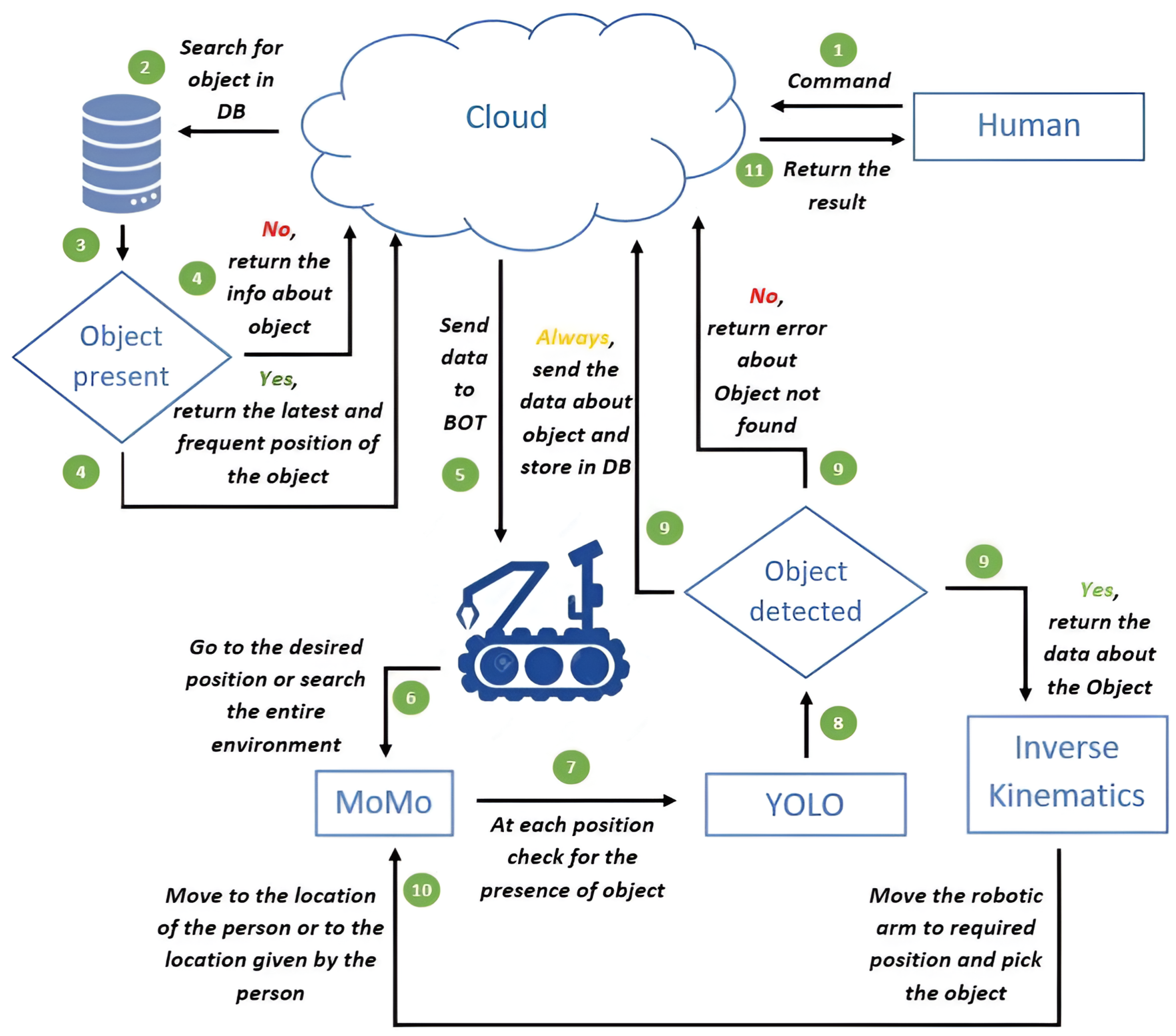Figure 17 depicts and illustrates the tasks performed by the robot from the perspective of the user.

The third phase is dedicated to relocating objects at uniform time intervals, initially set at 1 hour but adjustable based on the size of the environment. For larger environments, the time interval should be reduced, and vice versa. During this phase, the new positions of the objects are updated in the database. These three phases together form step 1, the “Preparatory Step”. The subsequent step is the “Searching Step”. When the consumer issues a search command for a specific object, the bot first looks for the object’s location in the database, a process referred to as “retrieval of data from DB”. Two types of locations are considered: the expected location and frequent locations. The expected location corresponds to the object’s recent known position, typically obtained during the “relocating objects” phase.

By analyzing the object’s overall movement history, the most frequent position where the object is often found is calculated. The bot begins by moving to the expected location, and if the object is detected there, it informs the consumer of its location. However, if the object is not found in the expected location, the bot proceeds to the most frequent location. If the object is still not detected, the bot enters the third phase, known as the “complete search”, where it thoroughly searches the environment for the object. In the “complete search” phase, the bot thoroughly scans the environment for the object. If the object is found, it informs the consumer about its location. If the object is not found, the bot informs the consumer that the required object cannot be located. The same phases and steps are followed for the “Take” command. In addition to the aforementioned steps, the bot picks up the object from the identified position and places it near the consumer’s location.

6. Results and Discussion

In this section, we present the obtained results for various algorithms. By examining the outcomes of the MoMo algorithm, the timing required for path planning in the environment is observed with the deployment of implemented algorithms in a real-time environment. The majority of the results align with our expectations and have received positive responses. However, a few results have provided us with valuable insights beyond our initial predictions. To compress the raw map, we employed the square box–square-region growth algorithm.

In Figure 18, the black boxes represent the obstacles present in the environment. The colored boxes, numbered accordingly, indicate the free area squares that are generated through the compression of the raw map. In a typical domestic environment, the average time required to find the optimal path for a minimum distance is less than 500 milliseconds.

Figure 19 illustrates a plot that demonstrates the exponential increase in time as the room area expands. As the algorithm is specifically designed for domestic environments, the average time required will always remain under 500 milliseconds. This graph also highlights the limitation of using this algorithm for larger environments exceeding the size of a typical house. The observations confirm the expected outcome with additional two parameters influencing the time required are the obstacle area and the distribution of obstacles within the environment, both of which are represented in the graph.

Table 1. Comparison of path lengths under different trails for the navigation of the mobile robotic manipulator to declutter objects.

Experiment Trails	ACO (cm)	PSO (cm)	Dijkstra (cm)	MoMo (cm)
Trail 1	452.72	485.31	428.23	421.37
Trail 2	453.43	485.85	429.47	420.65
Trail 3	459.57	484.28	428.14	421.85
Trail 4	453.46	485.91	429.36	420.9
Trail 5	451.02	487.83	428.15	420.04
Trail 6	458.48	483.72	429.47	420.78
Trail 7	457.65	486.64	428.68	421.65
Trail 8	456.15	485.23	427.96	421.21
Trail 9	454.86	485.64	427.92	420.97
Trail 10	455.94	483.58	428.27	420.95
Average	455.33	485.40	428.57	421.04

evaluates ACO, PSO, Dijkstra, and the proposed MoMo method in various experiment trials, highlighting the superior performance of our approach over conventional methods in minimizing the path length. Subsequently,

Table 2. Comparison of coverage times under different trails for the navigation of the mobile robotic manipulator to declutter objects.

Experiment Trails	ACO (s)	PSO (s)	Dijkstra (s)	MoMo (s)
Trail 1	22.64	25.54	21.41	16.85
Trail 2	22.67	25.57	21.47	16.83
Trail 3	22.98	25.49	21.41	16.87
Trail 4	22.67	25.57	21.47	16.84
Trail 5	22.55	25.68	21.41	16.80
Trail 6	22.92	25.46	21.47	16.83
Trail 7	22.88	25.61	21.43	16.87
Trail 8	22.81	25.54	21.40	16.85
Trail 9	22.74	25.56	21.40	16.84
Trail 10	22.80	25.45	21.41	16.84
Average	22.77	25.55	21.43	16.84

highlights the superior performance of MoMo approach in terms of minimum coverage time.

Based on the observations from Figure 20 and Figure 21, it is evident that the time taken for path planning is not consistent or precisely determinable due to the random distribution of obstacles within an environment. However, an approximation can be made. This finding also applies to the relationship between bounding box graphs and average time graphs. Moving on, let us discuss the results pertaining to the object detection algorithms.

Based on our extensive testing, the YOLO algorithm has demonstrated high efficiency and accuracy. The outcomes of the detection of various objects from the webcam mounted on the robotic manipulator using the YOLO object detection algorithm are shown in Figure 22. In comparison to other algorithms that we experimented with (like faster-CNN), YOLO has shown significant advantages. As mentioned earlier, the combination of YOLO and MoMo algorithms makes the robot well-suited for real-time domestic applications.

The plot depicted in Figure 23 illustrates a linear increase in time as the room area expands. This outcome aligns with our expectations, as it is a common behavior observed in various algorithms. Hence, the MoMo algorithm has demonstrated its efficiency and suitability for domestic environments.

7. Conclusions and Future Directions

A mobile robotic manipulator demonstrates tremendous potential, serving as a versatile and cost-effective home assistant that is capable of decluttering objects in both domestic and industrial settings. By leveraging deep learning techniques (such as YOLO) for accurate object detection, and incorporating inverse kinematics for precise positioning and movement of robotic arms, we successfully optimized grasp planning for efficient object decluttering. Additionally, the integration of our innovative MoMo algorithm, which utilizes odometry data, enhances the robot’s navigational capabilities within the environment. The MoMo path planning strategy outperformed state-of-the-art algorithms, achieving an average path length coverage of 421.04 cm in 10 trials and a faster average time of 16.84 s.

This robot’s implications extend beyond its decluttering capabilities. It can effectively support disabled and elderly individuals, acting as a valuable home assistant. Furthermore, in light of the coronavirus pandemic and the importance of social distancing, the robot offers a viable alternative to relying on human workers for domestic tasks. Integration with popular virtual assistants like Amazon Alexa, Google Home, and others, further enhances user experience, providing additional assistance and convenience. Affordability is another key advantage of this robot, as its low-cost nature makes it accessible to a wide range of individuals. This affordability is even more pronounced when considering the potential cost reduction achieved through bulk manufacturing. Furthermore, the robot’s versatility, cost-effectiveness, and ability to address current societal needs position it as a promising solution with significant prospects for the future. Future research in object decluttering will be focused on enhancing the adaptability and robustness of standard and novel meta-heuristic algorithms to address complex and dynamic scenarios in association with the MoMo approach.

References

1. Robinson, N.; Tidd, B.; Campbell, D.; Kulić, D.; Corke, P. Robotic vision for human-robot interaction and collaboration: A survey and systematic review. ACM Trans. Hum.-Robot. Interact. 2023, 12, 1–66. [Google Scholar] [CrossRef]
2. Lopez-Caudana, E.; Ramirez-Montoya, M.S.; Martínez-Pérez, S.; Rodríguez-Abitia, G. Using robotics to enhance active learning in mathematics: A multi-scenario study. Mathematics 2020, 8, 2163. [Google Scholar] [CrossRef]
3. Yao, K.; Billard, A. Exploiting Kinematic Redundancy for Robotic Grasping of Multiple Objects. IEEE Trans. Robot. 2023, 39, 1982–2002. [Google Scholar] [CrossRef]
4. Zarei, N.; Moallem, P.; Shams, M. Fast-Yolo-Rec: Incorporating yolo-base detection and recurrent-base prediction networks for fast vehicle detection in consecutive images. IEEE Access 2022, 10, 120592–120605. [Google Scholar] [CrossRef]
5. Schwarz, M.; Schulz, H.; Behnke, S. RGB-D object recognition and pose estimation based on pre-trained convolutional neural network features. In Proceedings of the 2015 IEEE International Conference on Robotics and Automation (ICRA), Seattle, WA, USA, 26–30 May 2015; IEEE: Piscataway, NJ, USA, 2015; pp. 1329–1335. [Google Scholar]
6. Yoshimoto, Y.; Tamukoh, H. Object recognition system using deep learning with depth images for service robots. In Proceedings of the 2018 International Symposium on Intelligent Signal Processing and Communication Systems (ISPACS), Ishigaki Island, Okinawa, Japan, 27–30 November 2018; IEEE: Piscataway, NJ, USA, 2018; pp. 436–441. [Google Scholar]
7. Su, H.; Zhang, Y.; Li, J.; Hu, J. The shopping assistant robot design based on ROS and deep learning. In Proceedings of the 2016 2nd International Conference on Cloud Computing and Internet of Things (CCIOT), Dalian, China, 22–23 October 2016; IEEE: Piscataway, NJ, USA, 2016; pp. 173–176. [Google Scholar]
8. Panić, B.; Klemenc, J.; Nagode, M. Improved initialization of the EM algorithm for mixture model parameter estimation. Mathematics 2020, 8, 373. [Google Scholar] [CrossRef]
9. Tung, T.X.; Ngo, T.D. Socially aware robot navigation using deep reinforcement learning. In Proceedings of the 2018 IEEE Canadian Conference on Electrical & Computer Engineering (CCECE), Quebec City, QC, Canada, 13–16 May 2018; IEEE: Piscataway, NJ, USA, 2018; pp. 1–5. [Google Scholar]
10. Xin, J.; Zhao, H.; Liu, D.; Li, M. Application of deep reinforcement learning in mobile robot path planning. In Proceedings of the 2017 Chinese Automation Congress (CAC), Jinan, China, 20–22 October 2017; IEEE: Piscataway, NJ, USA, 2017; pp. 7112–7116. [Google Scholar]
11. Tanwani, A.K.; Mor, N.; Kubiatowicz, J.; Gonzalez, J.E.; Goldberg, K. A fog robotics approach to deep robot learning: Application to object recognition and grasp planning in surface decluttering. In Proceedings of the 2019 International Conference on Robotics and Automation (ICRA), Montreal, QC, Canada, 20–24 May 2019; IEEE: Piscataway, NJ, USA, 2019; pp. 4559–4566. [Google Scholar]
12. Mahler, J.; Matl, M.; Liu, X.; Li, A.; Gealy, D.; Goldberg, K. Dex-net 3.0: Computing robust vacuum suction grasp targets in point clouds using a new analytic model and deep learning. In Proceedings of the 2018 IEEE International Conference on Robotics and Automation (ICRA), Brisbane, Australia, 21–25 May 2018; IEEE: Piscataway, NJ, USA, 2018; pp. 5620–5627. [Google Scholar]
13. Bouzoualegh, S.; Guechi, E.H.; Kelaiaia, R. Model predictive control of a differential-drive mobile robot. Acta Univ. Sapientiae Electr. Mech. Eng. 2018, 10, 20–41. [Google Scholar] [CrossRef]
14. Satish, V.; Mahler, J.; Goldberg, K. On-policy dataset synthesis for learning robot grasping policies using fully convolutional deep networks. IEEE Robot. Autom. Lett. 2019, 4, 1357–1364. [Google Scholar] [CrossRef]
15. Al-Qurashi, Z.; Ziebart, B. Hybrid algorithm for inverse kinematics using deep learning and coordinate transformation. In Proceedings of the 2019 Third IEEE International Conference on Robotic Computing (IRC), Naples, Italy, 25–27 February 2019; IEEE: Piscataway, NJ, USA, 2019; pp. 377–380. [Google Scholar]
16. Caldera, S.; Rassau, A.; Chai, D. Review of deep learning methods in robotic grasp detection. Multimodal Technol. Interact. 2018, 2, 57. [Google Scholar] [CrossRef]
17. Choi, C.; Schwarting, W.; DelPreto, J.; Rus, D. Learning object grasping for soft robot hands. IEEE Robot. Autom. Lett. 2018, 3, 2370–2377. [Google Scholar] [CrossRef]
18. Gordón, C.; Encalada, P.; Lema, H.; León, D.; Castro, C.; Chicaiza, D. Autonomous robot navigation with signaling based on objects detection techniques and deep learning networks. In Proceedings of the SAI Intelligent Systems Conference, London, UK, 5–6 September 2019; Springer: Berlin/Heidelberg, Germany, 2019; pp. 940–953. [Google Scholar]
19. Gan, L.; Grizzle, J.W.; Eustice, R.M.; Ghaffari, M. Energy-based legged robots terrain traversability modeling via deep inverse reinforcement learning. IEEE Robot. Autom. Lett. 2022, 7, 8807–8814. [Google Scholar] [CrossRef]
20. Ab Wahab, M.N.; Nefti-Meziani, S.; Atyabi, A. A comparative review on mobile robot path planning: Classical or meta-heuristic methods? Annu. Rev. Control 2020, 50, 233–252. [Google Scholar] [CrossRef]
21. Khan, A.H.; Li, S.; Cao, X. Tracking control of redundant manipulator under active remote center-of-motion constraints: An RNN-based metaheuristic approach. Sci. China Inf. Sci. 2021, 64, 1–18. [Google Scholar] [CrossRef]
22. Gao, W.; Tang, Q.; Ye, B.; Yang, Y.; Yao, J. An enhanced heuristic ant colony optimization for mobile robot path planning. Soft Comput. 2020, 24, 6139–6150. [Google Scholar] [CrossRef]
23. Chen, L.; Su, Y.; Zhang, D.; Leng, Z.; Qi, Y.; Jiang, K. Research on path planning for mobile robots based on improved ACO. In Proceedings of the 2021 36th Youth Academic Annual Conference of Chinese Association of Automation (YAC), Nanchang, China, 28–30 May 2021; IEEE: Piscataway, NJ, USA, 2021; pp. 379–383. [Google Scholar]
24. Lin, S.; Liu, A.; Wang, J.; Kong, X. An intelligence-based hybrid PSO-SA for mobile robot path planning in warehouse. J. Comput. Sci. 2023, 67, 101938. [Google Scholar] [CrossRef]
25. Xu, L.; Cao, M.; Song, B. A new approach to smooth path planning of mobile robot based on quartic Bezier transition curve and improved PSO algorithm. Neurocomputing 2022, 473, 98–106. [Google Scholar] [CrossRef]
26. Alshammrei, S.; Boubaker, S.; Kolsi, L. Improved Dijkstra algorithm for mobile robot path planning and obstacle avoidance. Comput. Mater. Contin 2022, 72, 5939–5954. [Google Scholar] [CrossRef]
27. Szczepanski, R.; Tarczewski, T. Global path planning for mobile robot based on Artificial Bee Colony and Dijkstra’s algorithms. In Proceedings of the 2021 IEEE 19th International Power Electronics and Motion Control Conference (PEMC), Gliwice, Poland, 25–29 April 2021; IEEE: Piscataway, NJ, USA, 2021; pp. 724–730. [Google Scholar]
28. Sahu, N.; Bhardwaj, R.; Shah, H.; Mukhiya, R.; Sharma, R.; Sinha, S. Towards development of an ISFET-based smart pH sensor: Enabling machine learning for drift compensation in IoT applications. IEEE Sens. J. 2021, 21, 19013–19024. [Google Scholar] [CrossRef]
29. Slim, M.; Rokbani, N.; Neji, B.; Terres, M.A.; Beyrouthy, T. Inverse Kinematic Solver Based on Bat Algorithm for Robotic Arm Path Planning. Robotics 2023, 12, 38. [Google Scholar] [CrossRef]
30. Macario Barros, A.; Michel, M.; Moline, Y.; Corre, G.; Carrel, F. A comprehensive survey of visual slam algorithms. Robotics 2022, 11, 24. [Google Scholar] [CrossRef]
31. Adibhatla, V.A.; Chih, H.C.; Hsu, C.C.; Cheng, J.; Abbod, M.F.; Shieh, J.S. Defect detection in printed circuit boards using you-only-look-once convolutional neural networks. Electronics 2020, 9, 1547. [Google Scholar] [CrossRef]
32. Devin, C.; Abbeel, P.; Darrell, T.; Levine, S. Deep object-centric representations for generalizable robot learning. In Proceedings of the 2018 IEEE International Conference on Robotics and Automation (ICRA), Brisbane, Australia, 21–25 May 2018; IEEE: Piscataway, NJ, USA, 2018; pp. 7111–7118. [Google Scholar]
33. Do, T.T.; Nguyen, A.; Reid, I. Affordancenet: An end-to-end deep learning approach for object affordance detection. In Proceedings of the 2018 IEEE International Conference on Robotics and Automation (ICRA), Brisbane, Australia, 21–25 May 2018; IEEE: Piscataway, NJ, USA, 2018; pp. 5882–5889. [Google Scholar]
34. Wang, Z.; Majewicz Fey, A. Deep learning with convolutional neural network for objective skill evaluation in robot-assisted surgery. Int. J. Comput. Assist. Radiol. Surg. 2018, 13, 1959–1970. [Google Scholar] [CrossRef]
35. das Mecês, W.O.; da Costa, E.M.; Tavares, J.W.; Diniz, P.P.; Torres, R.H. ROBTK: An intelligent robot to transport objects. In Proceedings of the Anais do VI Encontro Nacional de Computação dos Institutos Federais, SBC, Manaus, Brasil, 22–23 May 2019. [Google Scholar]
36. Albani, D.; Youssef, A.; Suriani, V.; Nardi, D.; Bloisi, D.D. A deep learning approach for object recognition with NAO soccer robots. In Proceedings of the Robot World Cup, Leipzig, Germany, July 2016; Springer: Berlin/Heidelberg, Germany, 2016; pp. 392–403. [Google Scholar]
37. Boroushaki, T.; Leng, J.; Clester, I.; Rodriguez, A.; Adib, F. Robotic grasping of fully-occluded objects using rf perception. In Proceedings of the 2021 IEEE International Conference on Robotics and Automation (ICRA), Xi’an, China, 30 May–5 June2021; IEEE: Piscataway, NJ, USA, 2021; pp. 923–929. [Google Scholar]
38. Pan, Z.; Zeng, A.; Li, Y.; Yu, J.; Hauser, K. Algorithms and systems for manipulating multiple objects. IEEE Trans. Robot. 2022, 39, 2–20. [Google Scholar] [CrossRef]
39. Khalid, S.; Alam, A.; Fayaz, M.; Din, F.; Ullah, S.; Ahmad, S. Investigating the effect of network latency on users’ performance in Collaborative Virtual Environments using navigation aids. Future Gener. Comput. Syst. 2023, 145, 68–76. [Google Scholar] [CrossRef]
40. Pan, Y.; Chen, C.; Zhao, Z.; Hu, T.; Zhang, J. Robot teaching system based on hand-robot contact state detection and motion intention recognition. Robot. Comput.-Integr. Manuf. 2023, 81, 102492. [Google Scholar] [CrossRef]
41. Wiesmann, L.; Guadagnino, T.; Vizzo, I.; Zimmerman, N.; Pan, Y.; Kuang, H.; Behley, J.; Stachniss, C. LocNDF: Neural Distance Field Mapping for Robot Localization. IEEE Robot. Autom. Lett. 2023, 8, 4999–5006. [Google Scholar] [CrossRef]
42. Liu, Z.; Zhang, Y.; Yu, X.; Yuan, C. Unmanned surface vehicles: An overview of developments and challenges. Annu. Rev. Control 2016, 41, 71–93. [Google Scholar] [CrossRef]
43. Do, V.T.; Pham, Q.C. Geometry-Aware Coverage Path Planning on Complex 3D Surfaces. arXiv 2023, arXiv:2303.03616. [Google Scholar] [CrossRef]
Figure 1. Overall working mechanism that delineates the step-by-step process of the algorithms, from the command input by the user to the final output generated by the bot.
Mathematics 11 04371 g001
Figure 2. Position of the optical sensor in the robot (upside down image).
Mathematics 11 04371 g002
Figure 3. Description of the robot with optical sensors and its axis.
Mathematics 11 04371 g003
Figure 4. At any time t, the robot may be at position Pp with angle θ p .
Mathematics 11 04371 g004
Figure 5. Comparison of 2 positions Pn and Pp.
Mathematics 11 04371 g005
Figure 6. Axis representation of the object at the initial and final positions.
Mathematics 11 04371 g006
Figure 7. Relative new position of the object in xp and yp axis.
Mathematics 11 04371 g007
Figure 8. Position without translation and with only the rotation of the axis.
Mathematics 11 04371 g008
Figure 9. The combined view of initial and final positions with the mouse axis.
Mathematics 11 04371 g009
Figure 10. Angular error deviation representation w.r.t. the position.
Mathematics 11 04371 g010
Figure 11. Linear error deviation representation w.r.t. the position.
Mathematics 11 04371 g011
Figure 12. Angular error representation w.r.t. time.
Mathematics 11 04371 g012
Figure 13. Linear error representation at stage n = 1 w.r.t. time.
Mathematics 11 04371 g013
Figure 14. Linear error representation at stage n = 2 w.r.t. time.
Mathematics 11 04371 g014
Figure 15. The designed mobile robotic manipulator and its functional components.
Mathematics 11 04371 g015
Figure 16. Dimensions of the developed mobile robotic manipulator.
Mathematics 11 04371 g016
Figure 17. Robot’s perspective of project tasks as perceived by the user.
Mathematics 11 04371 g017
Figure 18. The simulated outcome of Map generation and path planning using Dijkstra Algorithm.
Mathematics 11 04371 g018
Figure 19. Room area vs. average time taken for finding the path with minimum distance. The red line is the trend line.
Mathematics 11 04371 g019
Figure 20. Total obstacle area vs. average time taken for finding the path with minimum distance; the red line is the expected trend line.
Mathematics 11 04371 g020
Figure 21. Number of free area squares vs. average time taken for finding the path with minimum distance. The red line is the expected trend line.
Mathematics 11 04371 g021
Figure 22. Detection of various objects from the webcam using the YOLO object detection algorithm.
Mathematics 11 04371 g022
Figure 23. Analysis of the MoMo algorithm. Comparison of room area with the time taken to generate a complete raw map.
Mathematics 11 04371 g023