Adaptive Sliding Mode Attitude Tracking Control for Rigid Spacecraft Considering the Unwinding Problem

Abstract

Based on the unwinding problem caused by the dual valued property of the quaternion description method, this paper designs an anti-unwinding sliding mode adaptive attitude tracking control with external disturbances and inertia matrix uncertainty. The sliding mode surface used in this paper contains two equilibrium points and adopts an indirect method, which greatly reduces the computational complexity. The stability and anti-unwinding performance have been proven. The simulation results have verified the effectiveness of the control method and we have compared it with the general linear sliding mode. The results show that the control method proposed in this paper is more stable, has higher convergence accuracy and has anti-unwinding performance.

1. Introduction

With the continuous development of the aerospace industry, the structure of spacecraft is becoming increasingly complex, and the space environment is becoming increasingly harsh. The attitude control of spacecraft has always been of great concern. Up to now, there have been various control methods used to handle spacecraft attitude control problems. The relevant scholars at home and abroad have also conducted in-depth research on spacecraft attitude control based on modern control theory and technology, and have achieved many results, such as robust control [1], adaptive control [2,3], sliding mode control [4,5], and disturbance observer control [6,7,8].

In recent years, the application of sliding mode control (SMC) in spacecraft attitude control has gained increasing attention. SMC is a robust control method that can effectively handle the uncertainties and external disturbances encountered in spacecraft attitude control. The effectiveness of SMC for spacecraft attitude control has been extensively validated in both simulation and experimental studies. Ref. [9] uses the filtered error variable and indirect method for attitude tracking control, and considers actuator faults and actuator saturation simultaneously. In order to address the attitude stability problem of flexible spacecraft with uncertainty and interference, reference [10] proposes an SMC output feedback control law to solve the above problem. In [11], a sliding mode control method with fuzzy logic was proposed to handle the uncertainties and complex nonlinearities encountered in spacecraft attitude control. The simulation results showed that the proposed controller can achieve satisfactory tracking performance under various operating conditions. In [12], the authors proposed a sliding mode controller for spacecraft attitude tracking control, which can achieve fast and accurate tracking performance under various external perturbations. In order to overcome the singularity problem caused by sliding mode control, a terminal sliding mode control system is proposed in [13], which makes the system approach the terminal sliding mode surface in finite time. Combining the advantages of fast and nonsingular, ref. [14] proposes a fast nonsingular terminal sliding mode, while also considering actuator faults.

Overall, sliding mode control has shown great promise in addressing the challenges encountered in spacecraft attitude control. However, the “unwinding phenomenon” has not been considered. The “unwinding phenomenon” [15] refers to when an aerospace vehicle’s initial attitude is close to the desired attitude, and it does not rotate towards the desired attitude but instead rotates away from it, which results in unnecessary energy consumption of the vehicle. In order to avoid the singular problems caused by the three-parameter description, many scholars have done some work based on the quaternion method [11,16,17], but they did not consider the unwinding problem. Lee [18] designed a finite-time fault-tolerant control method based on an intermediate quaternion, which can make the system globally finite-time stable and anti-unwinding under external disturbances, inertial parameter uncertainties, and actuator failures. Hu designed a new set of attitude deviation functions and deviation vectors in [19] to deal with the problem of input saturation and attitude velocity limitations simultaneously, and the controller has anti-unwinding characteristics, but they did not consider actuator failures. To overcome the “unwinding phenomenon” caused by quaternion attitude representation, Kristiansen et al. [20] designed discontinuous feedback attitude control rates to simultaneously stabilize the two equilibrium points. Dong et al. [21] designed a new switching function using a hyperbolic sine function when the system state was limited to the switching surface. Then, based on this switching function, they designed a sliding mode attitude maneuvering controller to ensure the robustness of the closed-loop system to disturbances and inertial uncertainties, while solving the unwinding problem. The same sliding mode surface is also adopted in this paper.

In this paper, we design an adaptive sliding mode attitude tracking control in the presence of external interference and parameter uncertainty; the unwinding problem caused by the dual value of quaternion attitude description is also considered. The main contributions of this paper are as follows: (1) Unlike the linear sliding mode surface in [9], the sliding mode surface used in this paper contains two equilibrium points [20], making the attitude error system have anti-unwinding performance when it is in the sliding stage. (2) Unlike other methods that directly handle uncertainty itself, this paper uses an indirect method [9], which saves computational complexity, reduces the number of parameters in the control scheme, and makes it easier for engineering design. (3) The control scheme in this article has anti-unwinding performance, which enables the spacecraft to directly move towards the nearest desired attitude during attitude tracking, and saves on energy consumption.

The rest of the paper is organized as follows. In Section 2, the attitude tracking control problem description of rigid spacecraft is stated. In Section 3, a novel sliding mode surface is constructed, and the property of the sliding mode surface is analyzed. Furthermore, an unwinding-free adaptive sliding mode controller is presented, and the convergence property and unwinding-free performance of the closed-loop system are proven. In Section 4, simulation results and comparison are conducted to illustrate the efficiency of the proposed controller.

Notations: Throughout this paper, ${ℝ}^n$ denotes the sets of $n$-dimensional real vectors, and ${ℝ}^{n\times m}$ denotes $n\times m$ real number matrices, $I_n\in {ℝ}^{n\times n}$ is a unit matrix. In addition, for the $x\in ℝ$, the following two hyperbolic functions and their derivatives are used in this paper: $\sinh \left(x\right)=\frac{e^x-e^{-x}}{2}$, $\cosh \left(x\right)=\frac{e^x+e^{-x}}{2}$ and $\frac{d\cosh \left(x\right)}{dx}=\sinh \left(x\right)$, $\frac{darc\cos \left(x\right)}{dx}=-\frac{1}{\sqrt{1-x^2}}$.

2. Attitude Tracking Control Problem Formulation of Spacecraft

2.1. Attitude Kinematics and Dynamics for a Rigid Spacecraft

The spacecraft attitude kinematics and dynamics model under the quaternion attitude description method is [22]:

$${\dot{q}}_0=-\frac{1}{2}{q}_v^T\omega$$

(1a)

$${\dot{q}}_v=\frac{1}{2}\left(q_v^{\times }+q_0{I}_3\right)\omega$$

(1b)

$$J\dot{\omega }=-{\omega }^{\times }J\omega +\tau +d^{\prime }$$

(1c)

where $q={\left[q_0 q_v^T\right]}^T\in {ℝ}^4$ represents the attitude of the body frame ${\mathcal{F}}_b$ with respect to the inertia frame ${\mathcal{F}}_I$, $q_0$ is a scalar, and $q_v\in {ℝ}^3$ is a vector, satisfying $q_0^2+q_v^T{q}_v=1$; $\omega ={\left[{\omega }_1 {\omega }_2 {\omega }_3\right]}^T\in {ℝ}^3$ is the angular velocity of the spacecraft with respect to an inertial frame ${\mathcal{F}}_I$ and expressed in body frame ${\mathcal{F}}_b$; $J\in {ℝ}^{3\times 3}$ is the inertia matrix of the spacecraft expressed in ${\mathcal{F}}_b$, and this matrix is symmetric positive definite; $\tau \in {ℝ}^3$ and $d^{\prime }\in {ℝ}^3$ are the control torques and the external disturbances respectively; $I_3$ is the identity matrix; for vector $a={\left[a_1\hspace{0.33em}{a}_2\hspace{0.33em}{a}_3\right]}^T\in {ℝ}^3$, $a^{\times }$ denoted as a skewed symmetric matrix.

$$a^{\times }=\left[\begin{array}{ccc}0& -a_3& a_2\\ a_3& 0& -a_1\\ -a_2& a_1& 0\end{array}\right]$$

(2)

The quaternion of the rigid can also be described as

$$q=\left[\begin{array}{c}{q}_0\\ q_1\\ q_2\\ q_3\end{array}\right]=\left[\begin{array}{c}\cos \frac{\theta }{2}\\ e_1\sin \frac{\theta }{2}\\ e_2\sin \frac{\theta }{2}\\ e_3\sin \frac{\theta }{2}\end{array}\right]$$

(3)

where $\theta \in \left[0,2\pi \right]$ and $e={\left[e_1,e_2,e_3\right]}^T\in {ℝ}^3$ are the rotation angle and rotation axis of a rigid body.

Remark 1.

From the above Equation (3), it can be seen that there are two different descriptions of the same physical attitude. Traditional control methods only consider one of the two equilibrium points, which means that the state of the spacecraft system will move to this equilibrium point no matter how far away (although far away from the equilibrium point), which is the unwinding phenomenon. Therefore, the control scheme needs to acknowledge the unwinding problem and takes a corrective measure. The issue of two equilibrium points has been also studied in [23,24].

2.2. Attitude Error Kinematics and Dynamics for a Rigid Spacecraft

To address the attitude tracking issue, we define the relative quaternion $q_e={\left[q_{e0} q_{ev}^T\right]}^T$ as the relative orientation between the body frame and the desired frame with orientation $q_d={\left[q_{d0} q_{dv}^T\right]}^T$, which is

$$q_{ev}=q_{d0}{q}_v-q_0{q}_{dv}+q_v^{\times }{q}_{dv}$$

$$q_{e0}=q_{d0}{q}_0+q_{dv}^{\times }{q}_v$$

where $\Vert q_d\Vert =1$ and relative quaternion $q_e$ satisfies $\Vert q_e\Vert =q_{e0}^2+q_{ev}^T{q}_{ev}=1$. The rotational matrix $R$ is defined as $R=\left(q_{e0}^2-q_{ev}^T{q}_{ev}\right)I_3+2q_{ev}{q}_{ev}^T-2q_{e0}{q}_{ev}^{\times }$, and satisfies $\Vert R\Vert =1$, $\dot{R}=-{\omega }_e^{\times }R$. ${\omega }_e=\omega -R{\omega }_d$ is the relative angular velocity.

The relative quaternion $q_e={\left[q_{e0}{q}_{ev}^T\right]}^T$ and relative angular velocity ${\omega }_e$ can be defined as

$${\dot{q}}_{e0}=-\frac{1}{2}{q}_{ev}^T{\omega }_e$$

(4a)

$${\dot{q}}_{ev}=\frac{1}{2}\left(q_{ev}^{\times }+q_{e0}{I}_3\right){\omega }_e$$

(4b)

$$J{\dot{\omega }}_e=-{\omega }^{\times }J\omega +\tau +d^{\prime }+J\left({\omega }_e^{\times }R{\omega }_d-R{\dot{\omega }}_d\right)$$

(4c)

According to Euler’s rotation theorem as shown in [25], attitude error quaternion $q_e$ can be shown as $q_e={\left[\begin{array}{cc}\cos \frac{\theta \left(t\right)}{2}& e\sin \frac{\theta \left(t\right)}{2}\end{array}\right]}^T$.

As mentioned in [26], the inertia matrix $J$ consists of constant part $J_0$ and an uncertain part $\Delta J$, and $J$ can be written as $J=J_0+\Delta J$. Then, considering Equation (4c), we have

$$J_0{\dot{\omega }}_e=-{\left({\omega }_e+R{\omega }_d\right)}^{\times }{J}_0\left({\omega }_e+R{\omega }_d\right)+J_0\left({\omega }_e^{\times }R{\omega }_d-R{\dot{\omega }}_d\right)+\tau +d-\lambda q_{ev}$$

(5)

with

$$d=-{\left({\omega }_e+R{\omega }_d\right)}^{\times }\Delta J\left({\omega }_e+R{\omega }_d\right)-\Delta J{\dot{\omega }}_e+\Delta J\left({\omega }_e^{\times }R{\omega }_d-R{\dot{\omega }}_d\right)+d^{\prime }+\lambda q_{ev}$$

(6)

Remark 2.

$d$ is the total disturbance, which contains external disturbances and the nonlinearities of the system. As [9] pointed out, external disturbances are caused by solar radiation, magnetic force, gravity (which can be assumed to be bounded), and aerodynamic drag (proportional to the square of angular velocity). The nonlinearities of the system are determined by the desired attitude trajectory and physical parameters, especially the moment inertia. The reason for subtracting $\lambda q_{ev}$from Equation (5) and adding it to Equation (6) is for stability analysis convenience, which becomes clearer in the stability analysis section.

Assumption 1.

As pointed out in Remark 2, it is reasonable to assume that the disturbance d′ is bounded as $\Vert d^{\prime }\Vert \le c_1+c_2\Vert \omega {\Vert }^2$ and $\Vert {\omega }_d\Vert \le c_3$, $\Vert {\dot{\omega }}_d\Vert \le c_4$, $\Vert q_{dv}\Vert \le c_5$, $\Vert {\dot{q}}_{dv}\Vert \le c_6$, $\Vert \Delta J\Vert \le J_{\delta }$ with $c_i,\hspace{0.33em}i=1,2,\dots 6$ and $J_{\delta }$ unknown constants.

Note that $\Vert R\Vert =1$; it is straightforward to show that $\Vert {\omega }_e\Vert =\Vert \omega -R{\omega }_d\Vert \le \Vert \omega \Vert +c_w$ with $c_w$ unknown constant. It can be concluded that there exist several unknown constants $b_0\ge 0$, $b_1\ge 0$, $b_2\ge 0$ satisfying

$$\Vert d\Vert \le b_0+b_1\Vert \omega \Vert +b_2\Vert \omega {\Vert }^2\le b\Phi$$

(7)

$$\Phi =1+\Vert \omega \Vert +\Vert \omega {\Vert }^2$$

(8)

where $b\ge 0$ and $b=\max \left\{b_0,b_1,b_2\right\}$.

2.3. The Unwinding Phenomenon

The “unwinding phenomenon” in spacecraft attitude control refers to [15,27]: when the system is in certain specific initial states, despite the fact that the starting point of the attitude motion trajectory is close to the desired attitude balance point, under the control law, the attitude trajectory first moves away from the desired attitude, rotates through an angle of more than 180 degrees, and then returns to the vicinity of the balance point. This results in tasks that require only small attitude maneuvering requiring large-angle rotation to complete, leading to waste of control energy.

2.4. Control Objective

The control objective is to propose a sliding mode adaptive anti-unwinding attitude tracking control method in the presence of external disturbances and inertial uncertainties. The control scheme ensures that all state signals of the spacecraft system are uniformly ultimately bounded and there is no unwinding phenomenon during the attitude tracking process.

3. Controller Design

3.1. Sliding Mode Surface Design

For the rigid spacecraft, to develop the control scheme, we design the sliding mode surface [21]:

$$S={\omega }_e+\lambda Q_e$$

(9)

$$Q_e=\sinh \left(q_{e0}\right)q_{ev}$$

(10)

where $\lambda$ is a positive constant, then a theorem is given to prove that the control objective is achieved when the system states are restricted to the switching surface $S=0$.

Based on the characteristics of hyperbolic sine function and hyperbolic cosine function, the following lemmas and properties are used in the designing and stability proof of the spacecraft.

Properties 1.

(1) The maximal value of the function $\cosh q_{e0}$ can be obtained when $q_{e0}=1$ or $q_{e0}=-1$. (2) For $\theta \left(t\right)\in \left(0,\pi \right]$, there holds $\sinh \left(\cos \frac{\theta \left(t\right)}{2}\right)\ge 0$, and for $\theta \left(t\right)\in \left(\pi ,2\pi \right]$, there holds $\sinh \left(\cos \frac{\theta \left(t\right)}{2}\right)<0$.

Lemma 1.

Consider spacecraft systems (1) and (4). If sliding mode surface $S=0$, then ${\omega }_e\to 0$, $q_{e0}\to 1\hspace{0.33em}or\hspace{0.33em}-1$, and the unwinding phenomenon is avoided when attitude error system (4) is in the sliding stage.

Proof. 

First, we choose the following Lyapunov function:

$$V_1\left(t\right)=2\left(\max \left(\cosh q_{e0}\right)-\cosh q_{e0}\right)$$

(11)

By taking a time derivative of (11), we can get

$${\dot{V}}_1\left(t\right)=-2{\dot{q}}_{e0}\sinh q_{e0}$$

Substituting (4a) into above equation, we obtain

$$\begin{gathered} {\dot{V}}_1\left(t\right)\hspace{1em}\hspace{1em}\hspace{1em}=q_{ev}^T{\omega }_e\sinh q_{e0} \\ \hspace{1em}\hspace{1em}\hspace{1em}\hspace{1em}\hspace{1em}\hspace{1em}\hspace{1em}={\left(\sinh \left(q_{e0}\right)q_{ev}\right)}^T{\omega }_e \\ \hspace{1em}\hspace{1em}\hspace{1em} =-\lambda Q_e^T{Q}_e \\ \le 0 \end{gathered}$$

(12)

From the above equation, we can see that if ${\dot{V}}_1\left(t\right)=0$, there obtains $q_{e0}=0$ or $q_{ev}=0$.

When $q_{e0}=0$, combining with $\Vert q_e\Vert =1$, we obtain $q_{ev}^T{q}_{ev}=1$;

When $q_{ev}=0$, combining with $\Vert q_e\Vert =1$, we obtain $q_{e0}=\pm 1$.

Overall, we can get

$${\dot{V}}_1\left(t\right) {|}_{q_{e0}=0} ={\dot{V}}_1\left(t\right) {|}_{q_{e0}=1} ={\dot{V}}_1\left(t\right) {|}_{q_{e0}=-1} =0$$

(13)

Moreover, it can be obtained from (11) that

$$V_1\left(t\right) {|}_{q_{e0}=1} =V_1\left(t\right) {|}_{q_{e0}=-1} =0,\hspace{0.33em}{V}_1\left(t\right) {|}_{q_{e0}=0} \ne 0$$

(14)

Furthemore, for any small positive value $\varsigma$, it is obtained from (12) that ${\dot{V}}_1\left(t\right) | q_{e0}=\varsigma <0$. This, with the relations in (13) and (14), implies that $q_{e0}\to 1\hspace{0.33em}or\hspace{0.33em}-1$ on the switching surface $S=0$. In addition, substituting $q_{ev}=0$ into (9) gives ${\omega }_e=0$. Thus, the conclusion ${\omega }_e\to 0$, $q_{e0}\to 1\hspace{0.33em}or\hspace{0.33em}-1$ in Lemma 1 is proven.

Next, the unwinding-free performance of the attitude error dynamics (4) with the system states being on the switching surface $S=0$ is proven. According to $q_{e0}=\cos \left(\frac{\theta \left(t\right)}{2}\right)$, the Lyapunov function (11) can be rewritten as $S=0$

$$V_1=2\left(\max \left(\cosh q_{e0}\right)-\cosh \hspace{0.33em}\cos \frac{\theta \left(\mathrm{t}\right)}{2}\right)$$

(15)

Consequently, $S=0$

$${\dot{V}}_1=\dot{\theta }\left(t\right)\sin \frac{\theta \left(t\right)}{2}\sinh \cos \frac{\theta \left(t\right)}{2}$$

(16)

Note that, for functions $\sin \frac{\theta \left(t\right)}{2}$ and $\mathrm{sinhcos}\frac{\theta \left(t\right)}{2}$, $\sin \frac{\theta \left(t\right)}{2}>0$ when $\theta \left(t\right)\in \left(0,2\pi \right)$; $\sinh \cos \frac{\theta \left(t\right)}{2}\ge 0$ when $\theta \left(t\right)\in \left(0,\pi \right]$; $\sinh \cos \frac{\theta \left(t\right)}{2}<0$ when $\theta \left(t\right)\in \left(\pi ,2\pi \right)$. Then from Equations (12) and (16), we can get $\dot{\theta }\left(t\right)\le 0$ when $\theta \left(t\right)\in \left(0,\pi \right]$, and $\dot{\theta }\left(t\right)\ge 0$ when $\theta \left(t\right)\in \left(\pi ,2\pi \right)$.

Then, there hold

$$\underset{t\to \infty }{\lim }\theta \left(t\right)=\left\{\begin{array}{c}0,\theta \left(t_{s0}\right)\in \left(0,\pi \right]\\ 2\pi ,\theta \left(t_{s0}\right)\in \left(\pi ,2\pi \right)\end{array}\right.$$

(17)

This implies that the unwinding phenomenon is avoided when the system states are restricted to the switching surface $S=0$. $\square$

3.2. Anti-Unwinding Adaptive Sliding Mode Attitude Tracking Control Law Design and Convergence Analysis

Theorem 1.

Considering a rigid spacecraft (1) with the error dynamics (4), for expected attitude trajectory $q_d$,  $w_d$ under Assumption 1 and the proposed anti-unwinding adaptive sliding mode control scheme (18)–(22). By selecting appropriate design parameters, it can be ensured that all signals in the closed-loop system remain bounded.

$$\tau =-\left(k_0+\kappa \left(t\right)\right)S+{\omega }^{\times }{J}_0\omega -\lambda J_0{\dot{Q}}_e-J_0\left({\omega }_e^{\times }R{\omega }_d-R{\dot{\omega }}_d\right)$$

(18)

$$\kappa \left(t\right)=\frac{\widehat{b}\Phi }{\Vert S\Vert +\epsilon }$$

(19)

$$\epsilon =\frac{\mu }{1+\Phi }$$

(20)

$${\dot{Q}}_e=\frac{1}{2}\left(\sinh \left(q_{e0}\right)\left(q_{e0}{I}_3+q_{ev}^{\times }\right){\omega }_e-\cosh \left(q_{e0}\right)q_{ev}^T{\omega }_e{q}_{ev}\right)$$

(21)

where $k_0>0$, $\mu >0$ are chosen by the designer. $\widehat{b}$ estimates the upper bound $b$, and is designed as

$$\dot{\widehat{b}}=-k_1\widehat{b}+k_2\frac{\Vert S{\Vert }^2\Phi }{\Vert S\Vert +\epsilon }$$

(22)

where $k_1>0$, $k_2>0$ are design parameters.

Proof. 

Consider the following Lyapunov function:

$$V=\frac{1}{2}{S}^T{J}_{0}S+\frac{1}{2k_2}{\tilde{b}}^2+\lambda \left[q_{ev}^T{q}_{ev}+{\left(1-q_{e0}\right)}^2\right]$$

(23)

where $\tilde{b}=b-\widehat{b}$ is the estimation error; by taking a time derivative of (23) and the condition $S=0$, and control scheme (18)–(22), we get

$$\begin{array}{lll}\dot{V}& =& S^T{J}_0\dot{S}-\frac{1}{k_2}\tilde{b}\dot{\widehat{b}}+\lambda q_{ev}^T{\omega }_e\\ & =& S^T\left[-{\left({\omega }_e+R{\omega }_d\right)}^{\times }{J}_0\left({\omega }_e+R{\omega }_d\right)+J_0\left({\omega }_e^{\times }R{\omega }_d-R{\dot{\omega }}_d\right)+\tau +d\right.-\lambda q_e\\ & & +\left.\frac{1}{2}\lambda J_0\left(\sinh \left(q_{e0}\right)\left(q_{e0}{I}_3+q_{ev}^{\times }\right){\omega }_e-\cos \mathrm{h}\left(q_{e0}\right)q_{ev}^T{\omega }_e{q}_{ev}\right)\right]-\frac{1}{k_2}\tilde{b}\dot{\widehat{b}}+\lambda q_{ev}^T{\omega }_e\\ & =& -\left(k_0+\kappa \left(t\right)\right)S^{T}S+S^{T}d+\frac{1}{k_2}\tilde{b}\left(-\dot{\widehat{b}}\right)-{\lambda }^2{q}_e^T{q}_e\\ & \le & -k_0{S}^{T}S-\kappa \left(t\right)\Vert S{\Vert }^2+\Vert S\Vert b\Phi +\frac{1}{k_2}\tilde{b}\left(-\dot{\widehat{b}}\right)-{\lambda }^2{q}_e^T{q}_e\\ & =& -k_0{S}^{T}S-{\lambda }^2{q}_e^T{q}_e-\frac{\widehat{b}\Phi }{\Vert S\Vert +\epsilon }\Vert S{\Vert }^2+\Vert S\Vert b\Phi +\frac{1}{k_2}\tilde{b}\left(-\dot{\widehat{b}}\right)\end{array}$$

(24)

For $\forall \epsilon \ge 0$, $\frac{\Vert S\Vert }{\Vert S\Vert +\epsilon }\le 1$, and for $\forall \Phi \ge 0$, $\frac{\Vert \Phi \Vert }{\Vert \Phi \Vert +\epsilon }\le 1$, so we get

$$\begin{array}{ll}\dot{V}& \le -k_0{S}^{T}S-{\lambda }^2{q}_e^T{q}_e+\frac{\Vert S{\Vert }^2\Phi }{\Vert S\Vert +\epsilon }\tilde{b}+\epsilon b\Phi +\frac{1}{k_2}\tilde{b}\left(k_1\widehat{b}-k_2\frac{\Vert S{\Vert }^2\Phi }{\Vert S\Vert +\epsilon }\right)\\ & \le -k_0{S}^{T}S-{\lambda }^2{q}_e^T{q}_e+\frac{\Vert S{\Vert }^2\Phi }{\Vert S\Vert +\epsilon }\tilde{b}+\epsilon b\Phi +\frac{k_1}{k_2}\tilde{b}\widehat{b}-\frac{\Vert S{\Vert }^2\Phi }{\Vert S\Vert +\epsilon }\tilde{b}\\ & \le -k_0{S}^{T}S-{\lambda }^2{q}_e^T{q}_e+\mu b+\frac{k_1}{k_2}\tilde{b}\widehat{b}\end{array}$$

(25)

Because

$$\begin{array}{ll}\frac{k_1}{k_2}\tilde{b}\widehat{b}& =\frac{k_1}{k_2}b\widehat{b}-\frac{k_1}{k_2}{\widehat{b}}^2\le \frac{k_1}{k_2}b\widehat{b}\\ & =-\frac{k_1}{2k_2}{\left(b-\widehat{b}\right)}^2+\frac{k_1}{2k_2}\left(b^2-{\widehat{b}}^2\right)\\ & \le -\frac{k_1}{2k_2}{\left(b-\widehat{b}\right)}^2+\frac{k_1}{2k_2}{b}^2\end{array}$$

(26)

Substituting Equation (26) into Equation (25) yields

$$\begin{array}{ll}\dot{V}& \le -k_0{S}^{T}S-{\lambda }^2{q}_e^T{q}_e-\frac{k_1}{2k_2}{\tilde{b}}^2+\frac{k_1}{2k_2}{b}^2+\mu b\\ & \le -CV+{\epsilon }_0\end{array}$$

(27)

where $C=\min \left\{\frac{2k_0}{J_0},\lambda ,k_1\right\}>0$, ${\epsilon }_0=\frac{k_1}{2k_2}{b}^2+\mu b+\lambda {\left(1-q_{e0}\right)}^2<\infty$.

According to the bounded theorem in [28], we can conclude that $S,\hspace{0.33em}{q}_e$ and $\tilde{b}$ are uniformly ultimately bounded (UUB). Therefore, the control scheme can ensure that all signals in the spacecraft system are UUB.

The anti-winding performance of the proposed control scheme (18)–(22) can be obtained through the following derivation.

$${\dot{q}}_{e0}=\frac{1}{2}\lambda q_{ev}^T{q}_{ev}\sinh \left(q_{e0}\right)$$

(28)

From (28) and properties of $\sinh q_{e0}$, we can easily see that ${\dot{q}}_{e0}\ge 0,q_{e0}\to +1$ when $q_{e0}\ge 0$; ${\dot{q}}_{e0}<0,q_{e0}\to -1$ when $q_{e0}<0$. So, the proposed control scheme has anti-winding performance. The proof is completed. $\square$

Remark 3.

From the control scheme (18)–(22), it can be seen that although many variables are assumed to be bounded, the proposed control scheme in this paper only involves simple functions and variables. Therefore, compared to some existing methods [29,30,31], this control scheme requires less computational power, which makes it feasible even in practical engineering applications.

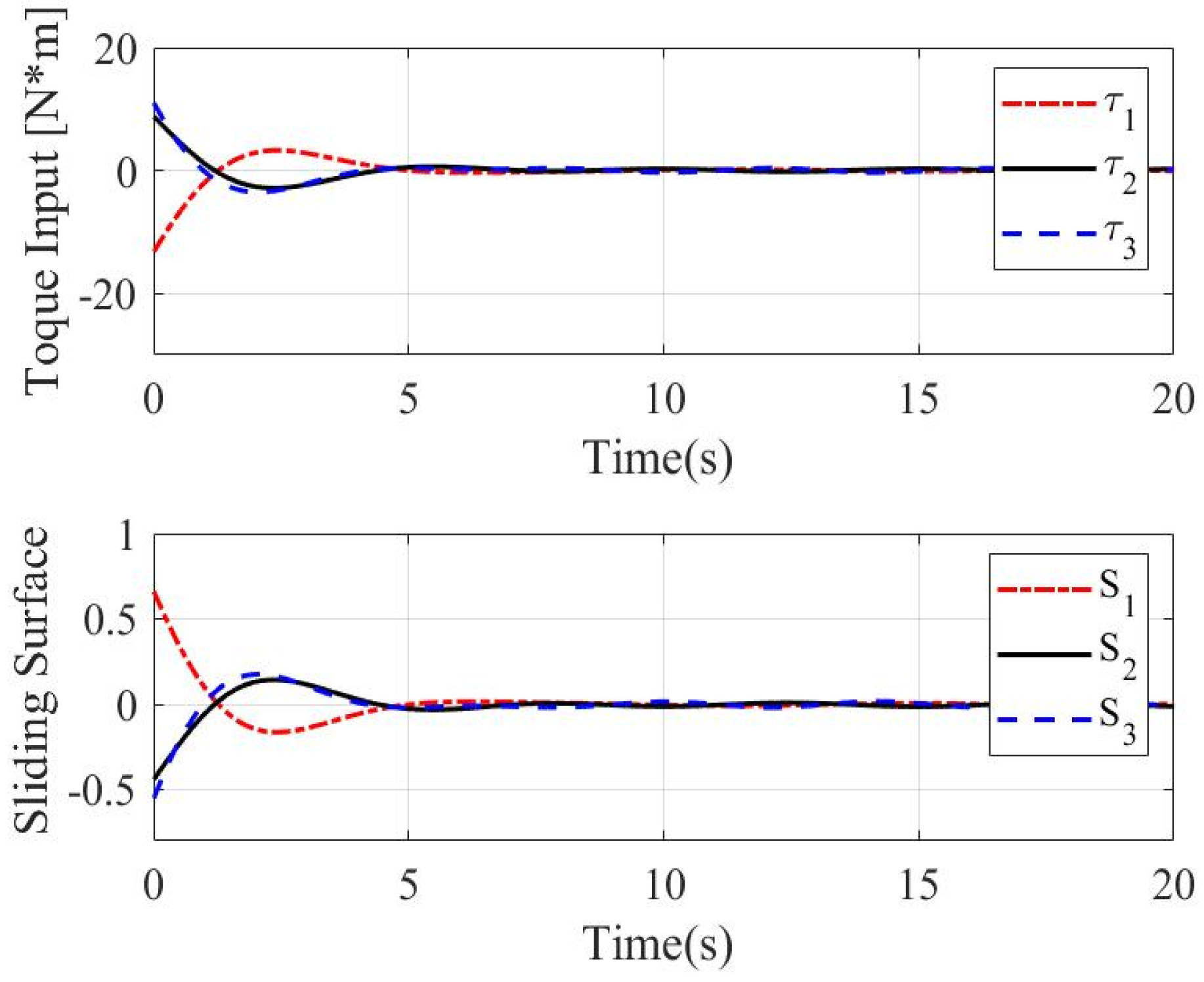
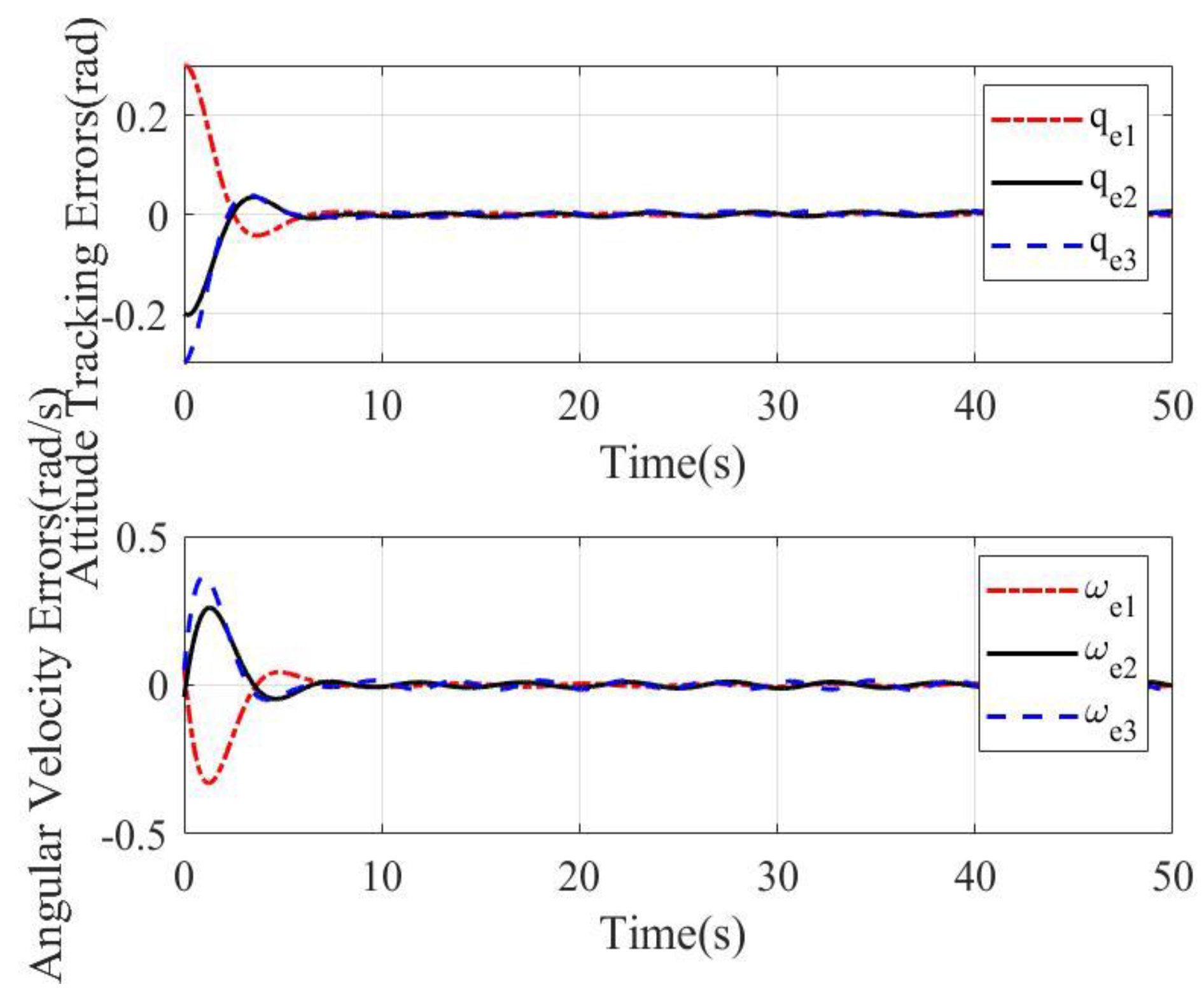
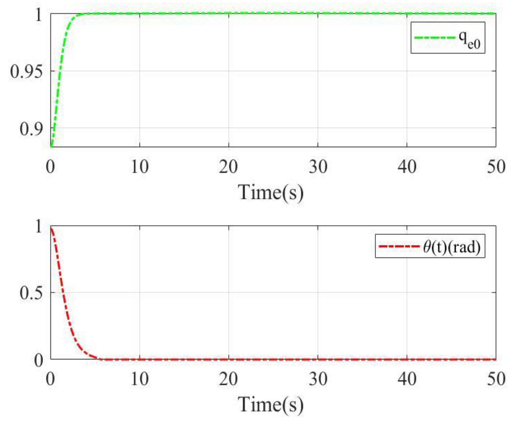
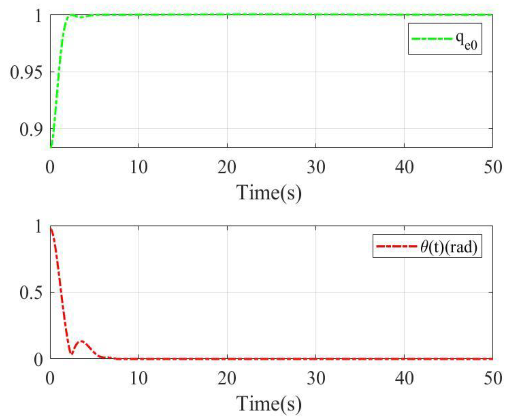
4. Simulation Results

This section provides a numerical simulation analysis of the proposed control strategy for a rigid spacecraft under external disturbances. To demonstrate the effectiveness of the designed control scheme, the performance of the proposed control scheme is also compared with the control algorithm proposed by [9], which uses a linear sliding mode and in which the unwinding issue has not been addressed. The linear sliding mode surface is $S={\omega }_e+\lambda q_{ev}$ and the main rigid parameters, moment of inertia, external interference, and control parameters remain the same; the linear SMC is $\tau =-\left(k_0+\kappa \left(t\right)\right)S$.

The nominal part and uncertainty of inertia matrix $J_0$ and $\Delta J$ [17] used in this paper are

$$J_0=\left[\begin{array}{ccc}20& 1.2& 0.9\\ 1.2& 17& 1.4\\ 0.9& 1.4& 15\end{array}\right],\Delta J=\left[\begin{array}{ccc}\sin 0.1t& 0& 0\\ 0& 2\sin 0.2t& 0\\ 0& 0& 3\sin 0.3t\end{array}\right]$$

The external disturbance acting on the rigid body is $d^{\prime }={\left[0.1\sin t 0.2\sin 1.2t 0.3\sin 1.5t\right]}^T$.

The desired trajectory and initial conditions of closed-loop parameters are listed in

Table 1. The desired trajectory and initial conditions of closed-loop parameters.

Variables	Values
${\omega }_d\left(t\right)$	${\left[\begin{array}{ccc}0.05\sin \frac{\pi t}{100},& 0.05\sin \frac{2\pi t}{100},& 0.05\sin \frac{3\pi t}{100}\end{array}\right]}^T$
$\omega \left(0\right)$ $q_e\left(0\right)$ $\widehat{b}\left(0\right)$	${\left[\begin{array}{ccc}0.06& -0.04& 0.05\end{array}\right]}^T$ ${\left[\begin{array}{cccc}-0.8832& 0.3& -0.2& -0.3\end{array}\right]}^T$ 0

. The control parameters of the control scheme are shown in

Table 2. The control parameters.

Variables	Values
$\lambda$	2
$\mu$	0.1
$k_0$	20
$k_1$	0.01
$k_2$	100

.

The simulation analysis is performed for two cases of the constant part of quaternion error $q_e\left(0\right)$, which are shown in

Table 3. Two cases of relative attitude.

Case	${\mathbf{q}}_{\mathbf{e}}\left(0\right)$
1	${\left[\begin{array}{cccc}0.8832& 0.3& -0.2& -0.3\end{array}\right]}^T$
2	${\left[\begin{array}{cccc}-0.8832& 0.3& -0.2& -0.3\end{array}\right]}^T$

. The initial conditions are the same in both cases, with the only difference being the polarity of the relative constant part of the quaternion. Therefore, the problem of unwinding will appear if it is not handled.

4.1. Case 1

The time response of control input $\tau$ and sliding surface $S$ with the sliding mode surface (9)–(10) designed in this paper and linear sliding mode described in [9] are shown in Figure 1 and Figure 2. As shown in Figure 1, the control input becomes stable at about 6 s, and the sliding surface converges to 0 in 4 s. As shown in Figure 2, the control input becomes stable at about 12 s, and the sliding surface converges to 0 in 12 s. Obviously, the proposed sliding mode $S$ in this paper can offer a faster response, better stability and higher accuracy for rigid body systems.

Attitude tracking errors and angular velocity errors with the sliding mode surface (9)–(10) designed in this paper and linear sliding mode in [9] are shown in Figure 3 and Figure 4, respectively. As shown in Figure 3, the attitude tracking errors and angular velocity errors with the sliding mode surface (9)–(10) become stable at about 5 s. As shown in Figure 4, attitude tracking errors and angular velocity errors with linear sliding mode become stable at about 15 s. Obviously, that depicted in Figure 3 can offer a faster response, better stability, and higher accuracy for rigid body systems.

The constant part of the quaternion error and rotation angle with two sliding mode surfaces are shown in Figure 5 and Figure 6. Since the initial condition of the relative scalar quaternion is positive in this case, the closest balance point is ${\left[1\hspace{0.33em}0\hspace{0.33em}0\hspace{0.33em}0\right]}^T$. As shown in Figure 5, under sliding mode surface (9)–(10) and control scheme (18)–(22), the constant part of quaternion error $q_{e0}$ reaches 1 and the rotation angle reaches 0 at about 4 s. As shown in Figure 6, under the linear sliding mode surface, the constant part of the quaternion error reaches 1 in 5 s and the rotation angle reaches 0 in about 10 s. Obviously, the proposed sliding mode $S$ in this paper can offer anti-unwinding performance for rigid body systems.

Adaptive law conditions are shown in Figure 7 and Figure 8. As shown in Figure 7 and Figure 8, the proposed control scheme can estimate an unknown parameter within 3 s, but within 10 s under the linear sliding mode surface. So, the control scheme (18)–(22) makes adaptive law have a faster response, better stability, and higher accuracy for rigid body systems.

4.2. Case 2

The time response of control input $\tau$ and sliding surface $S$ with the sliding mode surface (9)–(10) designed in this paper and linear sliding mode in [9] are shown in Figure 9 and Figure 10. As shown in Figure 9, the control input becomes stable at about 6 s, and the sliding surface converges to 0 in 4 s. As shown in Figure 10, the control input becomes stable at about 12 s, and the sliding surface converges to 0 in 12 s. Obviously, the proposed sliding mode $S$ in this paper can offer a faster response, better stability and higher accuracy for rigid body systems.

Attitude tracking errors and angular velocity errors with the sliding mode surface (9)–(10) designed in this paper and linear sliding mode in [9] are shown in Figure 11 and Figure 12, respectively. As shown in Figure 11, the attitude tracking errors and angular velocity errors with the sliding mode surface (9)–(10) become stable at about 5 s. As shown in Figure 12, attitude tracking errors and angular velocity errors with the linear sliding mode become stable at about 15 s. Obviously, Figure 11 can offer a faster response, better stability, and higher accuracy for rigid body systems.

The constant part of the quaternion error and rotation angle with two sliding mode surfaces are shown in Figure 13 and Figure 14, respectively. The initial condition of the constant part of the quaternion error is negative, so the closest equilibrium point is ${\left[-1\hspace{0.33em}0\hspace{0.33em}0\hspace{0.33em}0\right]}^T$. As shown in Figure 13, under sliding mode surface (9)–(10) and the control scheme (18)–(22), the constant part of quaternion error $q_{e0}$ reaches −1 and the rotation angle reaches $2\pi$ at about 4 s. As shown in Figure 14, under the linear sliding mode surface, the constant part of the quaternion error reaches 1 in 5 s and the rotation angle reaches 0 in about 10 s. Obviously, the proposed sliding mode $S$ in this paper can offer anti-unwinding performance for rigid body systems.

Adaptive law conditions are shown in Figure 15 and Figure 16. As shown in Figure 15 and Figure 16, the proposed control scheme can estimate an unknown parameter within 3 s, but within 10 s under a linear sliding mode surface. So, the control scheme (18)–(22) makes adaptive law have a faster response, better stability, and higher accuracy for rigid body systems.

Summarizing the above simulation results, it is obvious that the proposed controller in this paper satisfies the control objective and can achieve fast and accurate attitude tracking compared with a linear sliding mode surface, even in the presence of uncertainties and disturbances. This indicates that the control scheme has good robustness against internal uncertainties and external disturbances.

5. Conclusions

This article proposes a rigid spacecraft attitude tracking control method based on a sliding mode surface and adaptive control, which can effectively deal with the influence of parameter uncertainty and external interference on the spacecraft. This scheme uses indirect methods to handle uncertainty, has a simple structure and saves computational energy. By using Lyapunov theory to analyze the stability of the closed-loop system, the stability of the system is ensured. The simulation results show that the designed attitude tracking control scheme can effectively track the spacecraft attitude and has good robustness and anti-interference performance. Compared with existing methods, this controller has better performance indicators and wider application prospects. The limitation of this paper is that the finite time convergence and spacecraft actuator failures are not taken into consideration, which will be considered in the future.

References

1. Liu, C.; Ye, D.; Shi, K.; Sun, Z. Robust high-precision attitude control for flexible spacecraft with improved mixed H2/H control strategy under poles assignment constraint. Acta Astronaut. 2017, 136, 166–175. [Google Scholar] [CrossRef]
2. Sun, L.; Huo, W.; Jiao, Z. Adaptive backstepping control of spacecraft rendezvous and proximity operations with input saturation and full-state constraint. IEEE Tran. Ind. Electron. 2017, 64, 480–492. [Google Scholar] [CrossRef]
3. Chen, Z.; Huang, J. Attitude tracking and disturbance rejection of rigid spacecraft by adaptive control. IEEE Trans. Autom. Control 2009, 54, 600–605. [Google Scholar] [CrossRef]
4. Gao, Z.; Han, B.; Qian, M.; Lin, J. Active fault tolerant control for flexible spacecraft with sensor faults based on adaptive integral sliding mode. J. Nanjing Inst. Meteorol. 2018, 10, 146–152. [Google Scholar]
5. Li, Q.; Yuan, J.; Wang, H. Sliding mode control for autonomous spacecraft rendezvous with collision avoidance. Acta Astronaut. 2018, 151, 743–751. [Google Scholar] [CrossRef]
6. Sun, L.; Huo, W.; Jiao, Z. Disturbance observer-based robust relative pose control for spacecraft rendezvous and proximity operations under input saturation. IEEE Trans. Aerosp. Electron. Syst. 2018, 54, 1605–1617. [Google Scholar] [CrossRef]
7. Liu, Z.; Liu, J.; Wang, L. Disturbance observer based attitude control for flexible spacecraft with input magnitude and rate constraints. Aerosp. Sci. Technol. 2018, 72, 486–492. [Google Scholar] [CrossRef]
8. Xia, K.; Huo, W. Disturbance observer based fault-tolerant control for cooperative spacecraft rendezvous and docking with input saturation. Nonlinear Dyn. 2017, 88, 2735–2745. [Google Scholar] [CrossRef]
9. Cai, W.C.; Liao, X.H.; Song, Y.D. Indirect robust adaptive fault-tolerant control for attitude tracking of spacecraft. J. Guid. Control. Dyn. 2008, 31, 1456–1463. [Google Scholar] [CrossRef]
10. Hu, Q.L.; Ma, G.F. Control of three-axis stabilized flexible spacecraft using variable structure strategies subject to input nonlinearities. J. Vib. Control 2006, 12, 659–681. [Google Scholar] [CrossRef]
11. Huo, B.Y.; Xia, Y.Q.; Yin, L.J.; Fu, M.Y. Fuzzy Adaptive Fault-Tolerant Output Feedback Attitude-Tracking Control of Rigid Spacecraft. IEEE Trans. Syst. Man Cybern. Syst. 2017, 47, 8. [Google Scholar] [CrossRef]
12. Lu, K.F.; Xia, Y.Q. Adaptive attitude tracking control for rigid spacecraft with finite-time convergence. Automatica 2013, 49, 3591–3599. [Google Scholar] [CrossRef]
13. Feng, Y.; Yu, X.; Han, F. On nonsingular terminal sliding-mode control of nonlinear systems. Automatica 2013, 49, 1715–1722. [Google Scholar] [CrossRef]
14. Van, M.; Ge, S.S.; Ren, H. Finite time fault tolerant control for robot manipulators using time delay estimation and continuous nonsingular fast terminal sliding mode control. IEEE Trans. Cybern. 2017, 47, 1681–1693. [Google Scholar] [CrossRef] [PubMed]
15. Bhat, S.P.; Bernstein, D.S. A topological obstruction to continuous global stabilization of rotational motion and the unwinding phenomenon. Syst. Control Lett. 2000, 39, 63–70. [Google Scholar] [CrossRef]
16. Xia, Y.Q.; Fu, M.Y. Compound Control Methodology for Flight Vehicles; Springer: Berlin, Germany, 2013. [Google Scholar]
17. Huo, B.Y.; Xia, Y.Q.; Lu, K.; Fu, M.Y. Adaptive fuzzy finite-time fault-tolerant attitude control of rigid spacecraft. J. Frankl. Inst.-Eng. Appl. Math. 2015, 352, 4225–4246. [Google Scholar] [CrossRef]
18. Lee, D. Fault-tolerant finite-time controller for attitude tracking of rigid spacecraft using intermediate quaternion. IEEE Trans. Aerosp. Electron. Syst. 2020, 57, 540–553. [Google Scholar] [CrossRef]
19. Hu, Q.L.; Li, L. Anti-unwinding attitude control of spacecraft considering input saturation and angular velocity constraint. Actaeronautica Astronaut. Sin. 2015, 36, 1259–1266. [Google Scholar]
20. Kristiansen, R.; Nicklasson, P.; Gravdahl, J. Satellite attitude control by quaternion-based backstepping. IEEE Trans. Control Syst. Technol. 2009, 17, 227–232. [Google Scholar] [CrossRef]
21. Dong, R.Q.; Wu, A.G.; Zhang, Y. Anti-unwinding sliding mode attitude maneuver control for rigid spacecraft. IEEE Trans. Autom. Control 2022, 67, 978–985. [Google Scholar] [CrossRef]
22. Chen, Y.P.; Lo, S.C. Sliding-mode controller design for spacecraft attitude tracking maneuvers. IEEE Trans. Aerosp. Electron. Syst. 1993, 29, 1328–1333. [Google Scholar] [CrossRef]
23. Quoc, V.T.; Brian, D.O.A.; Hyo, S.A. Pose localization of leader–follower networks with direction measurements. Automatica 2020, 120, 109125. [Google Scholar]
24. Mouaad, B.; Abdelhamid, T. Bearing-Based Distributed Pose Estimation for Multi-Agent Networks. IEEE Control. Syst. Lett. 2023, 7, 2617–2622. [Google Scholar]
25. Shuster, M.D. A survey of attitude representations. Navigation 1993, 8, 439–517. [Google Scholar]
26. Zhu, Z.; Xia, Y.Q.; Fu, M.Y. Adaptive sliding mode control for attitude stabilization with actuator saturation. IEEE Trans. Industr. Electron. 2011, 58, 4898–4907. [Google Scholar] [CrossRef]
27. Liao, Y.; Yang, Y.J.; Wen, Y.L. Deformation Module Spaceeraft Attitude Control Techniques; National Defense Industry Press: Beijing, China, 2020. [Google Scholar]
28. Khalil, H. Nonlinear Systems; Prentice-Hall Press: Englewood Cliffs, NJ, USA, 2002. [Google Scholar]
29. Xiao, B.; Hu, Q.L.; Zhang, Y.; Huo, X. Fault-tolerant tracking control of spacecraft with attitude-only measurement under actuator failures. J. Guid. Control Dyn. 2014, 37, 838–849. [Google Scholar] [CrossRef]
30. Xu, B.; Huang, X.; Wang, D.; Sun, F. Dynamic surface control of constrained hypersonic flight models with parameter estimation and actuator compensation. Asian J. Control 2014, 16, 162–174. [Google Scholar] [CrossRef]
31. Lu, K.F.; Xia, Y.Q.; Fu, M.Y. Controller design for rigid spacecraft attitude tracking with actuator saturation. Inf. Sci. 2013, 220, 343–366. [Google Scholar] [CrossRef]
Figure 1. Control input and sliding surface with S (9)–(10) for case 1.
Mathematics 11 04372 g001
Figure 2. Control input and sliding surface under linear sliding mode for case 1.
Mathematics 11 04372 g002
Figure 3. Attitude tracking errors and angular velocity errors with sliding mode (9)–(10) for case 1.
Mathematics 11 04372 g003
Figure 4. Attitude tracking errors and angular velocity errors with linear sliding mode for case 1.
Mathematics 11 04372 g004
Figure 5. The constant part of quaternion error q e 0 and rotation angle θ with sliding mode (9)–(10) for case 1.
Mathematics 11 04372 g005
Figure 6. The constant part of quaternion error q e 0 and rotation angle θ with linear sliding mode for case 1.
Mathematics 11 04372 g006
Figure 7. Adaptive law with sliding mode (9)–(10) for case 1.
Mathematics 11 04372 g007
Figure 8. Adaptive law with linear sliding mode for case 1.
Mathematics 11 04372 g008
Figure 9. Control input and sliding surface with S (9)–(10) for case 2.
Mathematics 11 04372 g009
Figure 10. Control input and sliding surface under linear sliding mode for case 2.
Mathematics 11 04372 g010
Figure 11. Attitude tracking errors and angular velocity errors with sliding mode (9)–(10) for case 2.
Mathematics 11 04372 g011
Figure 12. Attitude tracking errors and angular velocity errors with linear sliding mode for case 2.
Mathematics 11 04372 g012
Figure 13. The constant part of quaternion error q e 0 and rotation angle θ with sliding mode (9)–(10) for case 2.
Mathematics 11 04372 g013
Figure 14. The constant part of quaternion error q e 0 and rotation angle θ with linear sliding mode for case 2.
Mathematics 11 04372 g014
Figure 15. Adaptive law with sliding mode (9)–(10) for case 2.
Mathematics 11 04372 g015
Figure 16. Adaptive law with linear sliding mode for case 2.
Mathematics 11 04372 g016