Abstract
To address an autonomous guided vehicle problem, this article presents extended variants of the established block over-relaxation method known as the Block Modified Two-Parameter Over-relaxation (B-MTOR) method. The main challenge in handling autonomous-driven vehicles is to offer an efficient and reliable path-planning algorithm equipped with collision-free feature. This work intends to solve the path navigation with obstacle avoidance problem explicitly by using a numerical approach, where the mobile robot must project a route to outperform the efficiency of its travel from any initial position to the target location in the designated area. The solution builds on the potential field technique that uses Laplace’s equation to restrict the formation of potential functions across operating mobile robot regions. The existing block over-relaxation method and its variants evaluate the computation by obtaining four Laplacian potentials per computation in groups. These groups can also be viewed as groups of two points and single points if they’re close to the boundary. The proposed B-MTOR technique employs red-black ordering with four different weighted parameters. By carefully choosing the optimal parameter values, the suggested B-MTOR improved the computational execution of the algorithm. In red-black ordering, the computational molecules of red and black nodes are symmetrical. When the computation of red nodes is performed, the updated values of their four neighbouring black nodes are applied, and conversely. The performance of the newly proposed B-MTOR method is compared against the existing methods in terms of computational complexity and execution time. The simulation findings reveal that the red-black variants are superior to their corresponding regular variants, with the B-MTOR approach giving the best performance. The experiment also shows that, by applying a finite difference method, the mobile robot is capable of producing a collision-free path from any start to a given target point. In addition, the findings also verified that numerical techniques could provide an accelerated solution and have generated a smoother path than earlier work on the same issue.
Keywords:
finite difference method; accelerated over-relaxation; Laplace’s equation; path navigation; optimal path; collision-free; block iterative schemes MSC:
65K05; 65K10; 35J05; 65M06; 65M22; 65N06; 65Y04
1. Introduction
The development of over-relaxation iterative methods families, in particular, Successive Over-Relaxation (SOR), Accelerated Over-Relaxation (AOR), and Two-Parameter Over-Relaxation (TOR), has sparked researchers’ interest in analyzing and solving numerous problems. These methods have been studied broadly in the past to solve linear system problems. The advent of the computer helps to solve elliptic partial differential numerically and efficiently using the SOR method [1]. In response to the significant role of SOR and the widespread use of this iterative technique, Hadjidimos [2] introduces a simple yet powerful scheme for a larger linear system called AOR. A decade later, ref. [3] established an extended scheme that fundamentally extends the AOR approach, known as the TOR method. The principle of block over-relaxation is applied to a novel type of block iteration in [4], and the resulting approach with a higher rate of convergence than that associated with single-line over-relaxation techniques was introduced. The block iteration approach was applied recently to solve the complex linear equations from the space fractional coupled nonlinear Schrodinger equations [5]. Apart from this, the block over-relaxation variants and their families have lately been utilized for quick computing [6,7,8,9,10,11].
In recent years, the study of path-planning exploitations, for instance, moving machines and autonomous agents, has gained a reputation in the research field. Formerly, refs. [12,13] introduced a global method for designing a smooth collision-free path through Laplace’s path planning equations. These two experiments demonstrate that harmonic functions provide a fast manner of constructing trails in a robot configuration region and prevent the emergence of local minima by chance. Following that, ref. [14] demonstrated the use of a numerical approach to address the path navigation issue, which concluded that by replicating complex problems with the maze, the new computational method of motion planning worked extremely well. Aside from that, refs. [15,16] have integrated iterative approaches with path-searching processes to tackle the path-finding problem in a global manner. Later, ref. [17] executed the application of potential functions for robot navigation. In accordance with his analyses, the end effector is subject to a repulsive force while every target exerts an appealing force. The harmonic potentials have also been expanded for a few other applications outside of autonomous robot path-planning, including ship navigation [18], space exploration [19], unmanned aerial vehicle planning [20], and marine maneuvers [21].
Autonomous robot navigation often involves discovering a collision-free path in a designated setting with obstacles to achieving a specific objective. The path-planning of a mobile robot in this study is performed using a numerical potential function in a predetermined environment, which is based on the heat transfer principle. The harmonic functions are the solutions to Laplace’s equation, notably used to solve the heat transfer problem. For the simulation of paths deriving from harmonic functions, temperature values in the defined area are employed. Computational approaches were utilized to generate harmonic functions owing to the availability of fast processing machines and the advanced algorithm to address the problem. In previous work, we have proved the value of the over-relaxation schemes and their variants in path-finding problems [11,22,23]. The positive outcomes of over-relaxation families’ iterative methods drive us to improve and provide an extension to the earlier work. Therefore, the core contribution of this article is the introduction of the newly iterative scheme of Block Modified Two-Parameter Over-relaxation (B-MTOR), which has been demonstrated to give faster convergence when optimal values are chosen. We conducted a variety of experiments to examine the effectiveness of iterative schemes for producing paths of mobile robots with varied obstacle figures in several sizes of environments.
2. Materials and Methods
We replicate the concept of driving a robot vehicle by means of a point that runs in an identified region rather than using the actual robot vehicle. The robot path planning can be illustrated as a steady-state heat transfer problem. The Laplace equation is frequently referred to as a steady-state heat equation [24] in the context of thermal conductivity, and its solutions are consistently denoted by harmonic functions. By resembling thermal conduction, the target point is to be regarded as a sink heat-pulling in, while the region border lines and all obstacles are kept at a constant temperature as it is identified as the heat source. The temperature distribution develops through the process of thermal conductivity, resulting in a thermal flux, which reflects the values of Laplacian potential, flowing into the sink that fills the configuration region. This can be interpreted as a way of interaction among the obstacles, goal location, and point robot. By observing the heat flux from high-temperature sources (with the highest potential value) to the lowest temperature point (with the lowest potential value) in the region, the field temperature distribution can then be utilized as a guide for the point robot as it moves from one location to another. Through the heat stream, it is simpler to view the path. This cycle, according to [12], guarantees a path to the target without running into local minima and certainly evades any barriers. By using the harmonic function to describe the environment setup, the temperature distribution of the configuration region is determined.
Mathematically, the harmonic function on domain bounded in region satisfies Laplace’s Equation (1), with the Cartesian coordinates of i-th denoted by , and n is the dimension. For the construction of the robot path in this study, the domain is composed of the region boundaries, initial positions, obstacles, and goal points.
The min-max rule holds true for harmonic functions; hence, it naturally follows that no local minima can suddenly occur in the solution domain [16]. Additionally, an escape path is always possible in every situation because the Gauss Integral Theorem [25] asserts that there is a balance between inward and outward flow on the boundary of any volume inside the solution domain (discounting the barriers and the target point). A harmonic function follows the min-max principle and has a gradient vector field with zero curls. Consequently, the only critical points that can arise are saddle points. A search in the area surrounding such a critical point can lead to the escape. Moreover, any path interference brought by such points yields a smooth path everywhere.
A robot in this model is characterized by a point in the configuration region. The region is built in a grid pattern, and each node’s coordinates and its function values are iteratively computed using the numerical approach. Various initial temperature values are given for the boundaries and obstacles, with the potential value appointed for the starting point set to high and the goal point being set as lowest. The Dirichlet constraint, , where c is constant, has been applied to Laplace’s equation solution. Once the harmonic function is founded within the boundary conditions, the suitable path can be positively found by trailing the heat stream executed through the gradient descent scheme (GDS) on calculated potential values. The descending search directs to the point with the smallest potential value, indicating the goal point. This descending manner is a sequence of points with lower potential values. The route’s streamline is determined by the coordinates and nodal temperature gradients obtained from the analysis of finite difference. In brief, the harmonic potentials are evaluated in the configuration region, including obstacles throughout the region and occupying the solutions to detect path lines for a mobile robot from an arbitrary initial point to a specific goal location. In general, the path-planning construction process in this study includes the following actions:
| Begin | |
| Step 1: Create a map of the robot’s region; | |
| Step 2: Initiate the formulation and modeling of the iterative schemes; | |
| Step 3: Formulate and execute the proposed iterative schemes algorithms; | |
| Step 4: Perform numerical simulations to obtain the solutions; | |
| Step 5: Evaluate the performances and algorithms complexity analysis. | |
| End |
2.1. Block Iterative Techniques
The block iterative schemes, also known as an explicit group (EG) iterative approach, were founded by [4]. All the algorithms in the block iterative methods family show that the evaluation is accelerated by obtaining four Laplacian potentials per computation. The calculation of groups of points that are close to the boundary is handled as groups of two points and a single point, as illustrated in Figure 1. This approach has been implemented in [11,22,23] to solve partial differential equation problems.
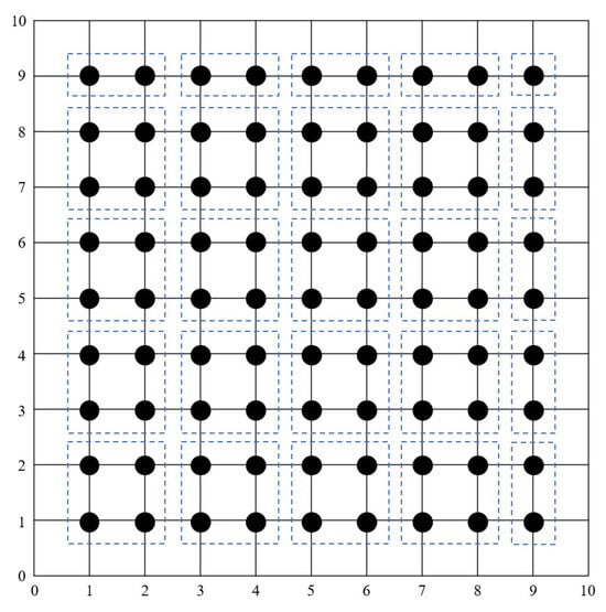
Figure 1.
Computational nodes for an explicit group iterative approach.
Eventually, the approximate values of the remaining node points for all block iterative methods are measured instantly through direct methods [26,27,28]. It is important to highlight that all algorithms used in this study are performed until the solution satisfies a specified convergence criterion, noted as . The stopping criterion utilized in this work is established on . Generally, implementations of all proposed iterative methods are typically imposed onto solid node points in Figure 1 until the convergence test criterion is fulfiled. With the exception of certain cases, especially the one near the boundary, all formulations utilizing the block iterative technique calculate a group of four nodes at once throughout the iteration process, refer to Figure 1. This block iterative approach, or the EG technique, is essentially generated using the standard five-point finite difference (5p-FD) approximation and is built on a group of a small number of points.
2.2. Red-Black Strategy
The red-black iterative approach, often referred to as red-black ordering, has been a fundamental technique used in numerical methods for solving partial differential equations and sparse matrix solvers for decades. In 1946, William [29] provided insights into the use of red-black ordering in solving linear systems of equations arising from Markov chain problems. It has evolved as a common and widely accepted technique. Studies on this approach can be found in the recent literature [30,31]. The formulations of the red-black ordering strategy for each of the modified variants are shown in Figure 2. The formulation concept of the red-black ordering strategy is as much the same as the corresponding explanation for nodal points in Figure 1, which has been briefly covered in the previous section.
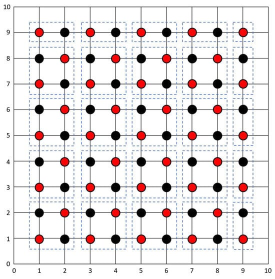
Figure 2.
The red-black strategy on the explicit group iterative approach, where the computational nodes are divided into red and black nodes. Half of the nodes are in red color and the other half are in black color.
The red–black approach uses two separate weighted parameters, and , for the respective red and black nodes to replace conventional parameter . Additionally, for the over-relaxation schemes, the accelerated parameter is shifted into two different accelerated parameters and . By giving a broader selection of values in the range between 1 and 2 and with appropriate parameter values, this approach will produce a suitable optimum iteration number and expedite the computational time. The proportion of the computational molecules for the red and black nodes, with the black node applying the updated values of its four adjoining red nodes and conversely, is readily visible in Figure 3. The red–black ordering strategy alternately computes the red and black nodes. Only red nodes will be computed in the first iteration, and only black nodes will be computed in the subsequent iteration; this process continuously calculates all the nodes in the region.
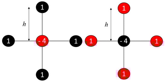
Figure 3.
Computational molecules for finite difference approximation (h represents the distance between node points in rectangular grid’s i and j directions). The molecules of red and black nodes are symmetrical, in which the black nodes applies the updated values of its four neighbouring red nodes, and vice versa.
2.3. Finite Difference Schemes
Consider the two-dimensional Laplace’s equation as set out in Equation (1) as
The standard second-order 5p-FD method, which is frequently used to represent the event of fluid dynamics and heat conduction processes, can be used to simplify the approximation of Equation (2), commonly stated as
This equation is then operated for the iterative methods executed on the grids. Accordingly, the iterative schemes for the standard 5p-FD formula can be written as
As mentioned previously, this study focuses on block over-relaxation iterative schemes for the proposed solver, i.e., SOR, AOR, TOR, and its modified variants, using explicit group technique. The standard iterative scheme for corresponding methods is necessary in order to implement the block iterative scheme. Therefore, from Equation (4), the standard SOR iterative schemes with relaxation parameter is expressed as
The AOR iterative technique, however, contains two relaxation parameters: and . Both parameters can be utilized to produce iterative methods that can accelerate the convergence rates, and AOR is more compliant and appropriate than any other method in this family. As defined by [2], to find the AOR iterative scheme for the standard five-point approximation, we switch and with and respectively, and insert the and terms. Hence, the AOR iterative scheme for the standard five-point formula on the grid can be written as
At the same time, the TOR iterative method represents a simplification of the AOR method, which involves three relaxation parameters: , , and . Obviously, if , the scheme of TOR is reduced to the AOR method. For both TOR and AOR methods, the parameters are selected to be close to the value of the corresponding SOR, and all of the parameters are expressed in the range of . The TOR iterative scheme for the standard five-point formula on the grid is written as
The implementation of these finite differences, Formulae (3) to (7), to approximate problem (2) will produce a large and sparse linear system that can be expressed in matrix form as
where A and b are known and u is unknown.
Standard Modified over Relaxation Schemes
The construction of formulation for the standard, modified SOR methods, namely Modified Successive Over-Relaxation (MSOR), can generally be expressed as
for red nodes. Whilst the black nodes are given as
Next, the formulation of standard, modified AOR methods, also known as Modified Accelerated Over-Relaxation (MAOR), can be written in red nodes as
while the black nodes are written as
Meanwhile, the standard, modified TOR methods, referred to as Modified Two-Parameter Over-Relaxation (MTOR), can be stated as
for red nodes, although black nodes can be stated as
3. Block over Relaxation Schemes
Let us take into consideration a set of four points (4 × 4), as illustrated in Figure 1, to make the formulation of the block SOR approach simpler. By reflecting the approximation in Equations (3) and (5), the block SOR method can be generally expressed as
where
By concluding the inverse of the coefficient matrix, Equation (15) can be amended as
where
Now, the block SOR iterative scheme for Equation (16) is revised to
In reality, the block MSOR (B-MSOR) iterative technique formulation is akin to that of the block SOR method but with an additional relaxation parameter. By employing the MSOR method in Equations (15)–(17), we are now referring to a group of four points (4 × 4) from Figure 2. The B-MSOR iterative scheme is typically stated as Equation (17) by taking into account the approximation in Equation (3) as well as from Equations (9) and (10) for red and black nodes, respectively.
The block AOR method’s formulation, in the meantime, evaluates the approximation equation from Equations (3) and (6) while also considering the node points in Figure 1. The AOR block scheme is then described as follows
where
Once again, Equation (18) can be converted into a linear system as Equation (8) and admitting the inverse of matrix A as in Equation (16). The block AOR iterative technique may now be generally expressed as Equation (17), although with different matrix elements S as revealed above in Equation (18).
Concurrently, considering computational nodes in Figure 1 with addressing Equations (3) and (7), the formulation of the block TOR method is written as
where
Red-Black Block Modified over Relaxation Schemes
The modified variants of AOR and TOR methods are capable of reducing to Jacobi extrapolation or modified SOR with certain sets of the acceleration and relaxation matrices by unique parameters corresponding to the row blocks of matrix A. All modified over-relaxation methods involve the execution of a red-black ordering strategy and using different additional relaxation parameters from others.
The formulation of the block MAOR (B-MAOR) iterative technique is also analogous to the block AOR method formulation with extra relaxation parameters. Consider the four points (4 × 4) in Figure 2; via the approximation from Equation (3) along with Equations (11) and (12), the B-MAOR iterative scheme can be generally described for red nodes as
where
and black nodes are presented as
with
Again, using Figure 2 as reference, and seeing the approximation in Equation (3) and from Equations (13) and (14). The inverse of the coefficient matrix for red nodes and black nodes of block MTOR (B-MTOR) iterative scheme can be expressed in general as same as Equations (20) and (21) except the S element in Equation (21) is written as
The , , , and are denoted as the optimal relaxation parameters for each formulation of over-relaxation variants. The ambiguous optimal values of the relaxation parameters did not constrain the minimum number of iterations. It is important to reiterate that the value of , , and are often chosen to be near to the value of the corresponding SOR, where , as evidently stated in [2]. All of these relaxation parameters in this study were determined using the sensitivity analysis practice, also known as parameter tuning. Furthermore, since the values of each parameter are predetermined before the execution, the influence of complexity on obtaining parameter value to overall computation remains constant. However, if the parameter value ranges are set in the algorithm computation, it will certainly change. Table A1 in the Appendix A gives a list of the optimal values used throughout experiments in this article.
Thus, the implementation of the red-black block MTOR scheme built on Equations (20) and (21) for solving two-dimensional Laplace’s problem as defined in Equation (2) can be expressed in Algorithm 1.
| Algorithm 1: Red-Black Block MTOR scheme. |
|
4. Numerical Results
In line with the study’s objectives, several experiments have been carried out with a robot 2D simulator [32] constructed by the authors to evaluate the efficiency of the suggested algorithm as a tool for resolving the path-planning issue. Additionally, the Java version of the simulator is available for download from [32]. The experiments were performed on an AMD A10 machine with 8 GB memory operating at 2.50 GHz. Up until the stopping criterion is reached, the iteration process to evaluate the temperature values numerically at all points continues. Additionally, the loop would be ended if there were no longer indicating changes in the temperature values, in which the difference in the measurement values was extremely small, i.e., . This level of accuracy was required in the solution to avoid saddle points, or flat areas, from interfering with the production of pathways.
Table 1 shows the iteration number and the execution time in seconds needed to compute every method used in the experiments. Clearly, the B-MTOR iterative method provided high performance compared with other proposed methods. At the same time, the iteration numbers for the modified families were slightly higher in the larger environment size than those for standard approaches.

Table 1.
Iterations number (k) and execution time (t) in seconds for the proposed iterative schemes. N × N is the size of the grid mesh, e.g., N = 300.
The output of the proposed approaches based on Table 1 is shown in the graphs in Figure 4 (the iteration number) and Figure 5 (the execution time). Both figures suggest that the length of each execution increases with the number of iterations. The graphs for the iteration number and execution time showed the same pattern, as can be seen in the results table. Although the iteration count for modified families varied slightly from that for conventional methods, depending on the region area, it appears that the red-black block MTOR iterative scheme provides significant efficiency in terms of time taken compared to other proposed approaches.
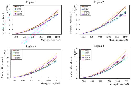
Figure 4.
Graph performance with respect to the iteration number.
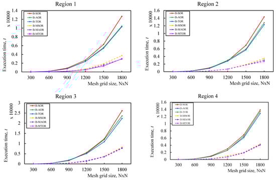
Figure 5.
Graph performance with respect to the execution time.
Computational Complexity
The computational complexity analysis of each iterative technique taken into consideration in this work is covered in this part. It is anticipated that each arithmetic operation (addition and multiplication) will separately take one unit of computational time. The GDS algorithm’s path-tracing process and the arithmetic operations are both disregarded by the convergence test. The total number of arithmetic operations involved by each of the examined approaches is listed in Table A2 in Appendix A.
The number of iterations should theoretically decrease as the algorithm’s computational complexity declines, saving CPU time. Families of the AOR method converge more quickly than families of the SOR method despite having more arithmetic operations owing to extra weighted parameters [3]. In the meantime, as the computation of the remaining points is only calculated in one iteration, it will be ignored from the total computation of computational complexity; hence, they will not significantly affect the overall computation.
5. Discussion
The stationary configuration regions, which included varying impediments in four separate regions with six distinct sizes, i.e., 300 × 300, 600 × 600, 900 × 900, 1200 × 1200, 1500 × 1500, 1800 × 1800, were tested in this study. High-temperature values are initially assigned to the obstacles and external boundaries. The target point was designated as having the lowest temperature, whereas the starting point had no initial value. The temperature value for the unoccupied space inside the regions was fixed to zero. The measurement of the temperature values proceeded numerically at each point before the stoppage circumstances were encountered. The loop terminates when the temperature values no longer show any changes, with iterations k and k + 1 having a very insignificant distinction between harmonic potentials, i.e., . This high level of accuracy was necessary to prevent route generation failures and steer clear of saddle points or flat areas in the configuration region.
The proper trail was yielded once the temperature values were obtained by using the steepest descent search from the starting point to the destination point. Figure A1 shows the successful pathways produced by numerical computation based on the acquired Laplacian potential in a predetermined stationary environment. All starting points (green square) were efficiently finished at the specified destination point (red circle), overcoming all types of obstacles in various regions. Some pathways appear jagged in some cases because no interpolation is performed. The idea is that gradient interpolation is supposed to provide smoother pathways. Figure A2 in the appendices displays the flow diagram for the path-planning technique used in this study.
The ideology of path-planning flow within this experiment starts with establishing the initial start point and the goal location. The next step is determining the ideal parameter corresponding to the proposed iterative schemes. Once the harmonic potential is generated from the selected algorithm, a completely smooth path is developed through the GDS technique. This impression could be used to represent an iterative scheme that follows a descending gradient from its starting point to subsequent consecutive points that have lower potentials than the preceding points all the way to the destination point (with the lowest potential value). Figure 5 provides observational evidence of these productive pathways, which shows every start point from every region successfully completed the path by reaching the destination point along with avoiding any walls and obstacles in between (if any). The paths’ trajectory can be extremely quick since it only involves the gradient evaluation of the precomputed Laplacian potential [12]. All four configuration regions in this experiment are relatively simple, referring to [33].
The enhanced version of potential field approaches has been explicitly implemented in Algorithm 1. In essence, the goal point and impediments function as charged surfaces, and the overall potential generates imaginary forces on the robot. This imaginary force attracts the robot toward the goal and keeps it away from obstacles [17]. Later, as the robot approaches its intended point, it will travel along the negative gradient to avoid every impediment. This study makes use of the harmonic function to avoid a local minima issue [16]. Furthermore, Algorithm 1 performs significantly better computing when the red-black block accelerated relaxation technique is implemented to solve the path-planning problem as it executes much faster in obtaining the solution of Laplace’s equation. Unmanned surface vehicles (USVs) are among the potential use cases for the provided approach in this study. In the past, ref. [34] has implemented a USV platform that uses a global positioning system compass for autonomous navigation in monitoring paddy growth. In addition, ref. [35] recently developed a USV navigation autopilot for disaster risk management, which has been used for environmental monitoring.
6. Conclusions
The red-black block modified scheme is used in conjunction with the iterative approaches from over-relaxation families to improve execution performance and reduce execution time. The newly proposed block MTOR iterative schemes perform more effectively due to the addition of accelerated weighted parameters to respective nodes, and the results are encouraging. The studies clearly prove that owing to cutting-edge algorithms and the present-day availability of fast machines, the robot path-planning problem is feasibly solved using numerical techniques. The block MTOR scheme is shown to greatly surpass its predecessor’s techniques in the table of results in the context of both iteration number and the time taken. Increasing the number of obstacles has no impact on the computational performance; in fact, the calculation will complete faster since it ignores the regions affected by the obstacles. The larger the space that impediments occupy, the less the calculations and storage are required; in other words, the obstacle eliminates the computing domain. It is not wrong to emphasise, once again, the block MTOR findings perform better than the block MSOR in terms of the iteration count (by 9-15%), while the block MTOR saves about 15-25% over block MSOR in terms of processing time. Simultaneously, the block TOR surpasses the block SOR by approximately 13-20% relating to iteration count and 11-18% concerning the execution time. It can also be inferred that block MTOR is equally competitive compared to block MAOR; however, block MTOR provides a wider range of parameters for fine-tuning optimization. Another uniqueness or novelty component of this study is the implementation of the red-black block overrelaxation scheme families in robot path planning and in Algorithm 1. To further the proposed approaches for future work, investigation into the half- [9,11,26,27] and quarter-sweep strategy [28,36,37,38] will be considered. It is anticipated that these approaches will improve the overall computation.
Author Contributions
Conceptualization, A.A.D.; methodology, A.A.D.; software, A.S.; validation, A.A.D., A.S. and J.S.; formal analysis, A.A.D.; investigation, A.A.D. and A.S.; resources, A.S. and J.S.; data curation, A.A.D. and J.S.; writing—original draft preparation, A.A.D. and A.S.; writing—review and editing, A.A.D., A.S. and J.S.; visualization, A.A.D.; supervision, A.S. and J.S.; project administration, A.S. and J.S.; funding acquisition, A.A.D. All authors have read and agreed to the published version of the manuscript.
Funding
This research was financially supported by Universiti Pertahanan Nasional Malaysia. The authors also acknowledge support from Science Foundation Ireland (SFI) under Grant Number SFI/16/RC/3918 (Confirm) and Marie Skłodowska-Curie grant agreement No. 847577 co-funded by the European Regional Development Fund for funding the APC.
Data Availability Statement
Not applicable.
Conflicts of Interest
The authors declare no conflict of interest.
Appendix A
Table A1.
Grid search of relaxation parameter values.
Table A1.
Grid search of relaxation parameter values.
| Methods | ||||
|---|---|---|---|---|
| B-SOR | 1.81 | - | - | - |
| B-MSOR | 1.83 | 1.81 | - | - |
| B-AOR | 1.81 | - | 1.84 | - |
| B-MAOR | 1.82 | 1.81 | 1.84 | - |
| B-TOR | 1.81 | - | 1.84 | 1.85 |
| B-MTOR | 1.80 | 1.81 | 1.84 | 1.85 |
Table A2.
Number of arithmetic operations per iteration for block over relaxation techniques and its modified variants methods.
Table A2.
Number of arithmetic operations per iteration for block over relaxation techniques and its modified variants methods.
| Methods | ADD/SUB | MUL/DIV |
|---|---|---|
| B-SOR/B-MSOR | ||
| B-AOR/B-MAOR | ||
| B-TOR/B-MTOR |
Appendix B


Figure A1.
Path creation from different starting points (square/green point) to the target positions (round/red point) in different region areas with percentage of free and occupied space in an identified stationary environment.
Figure A1.
Path creation from different starting points (square/green point) to the target positions (round/red point) in different region areas with percentage of free and occupied space in an identified stationary environment.


Figure A2.
Flow diagram of the path-planning technique.
Figure A2.
Flow diagram of the path-planning technique.

References
- Young, D.M. Iterative Methods for Solving Partial Difference Equations of Elliptic Type. Ph.D. Thesis, Harvard University, Cambridge, MA, USA, 1950. [Google Scholar]
- Hadjidimos, A. Accelerated overrelaxation method. Math. Comput. 1978, 32, 149–157. [Google Scholar] [CrossRef]
- Kuang, J.; Ji, J. A survey of AOR and TOR methods. J. Comput. Appl. Math. 1988, 24, 3–12. [Google Scholar] [CrossRef]
- Evans, D.J.; Biggins, M.J. The solution of elliptic partial differential equations by a new block over-relaxation technique. Int. J. Comput. Math. 1982, 10, 269–282. [Google Scholar] [CrossRef]
- Xiang, S.; Zhang, S. A convergence analysis of block accelerated over-relaxation iterative methods for weak block H-matrices to partition π. Linear Algebra Appl. 2006, 418, 20–32. [Google Scholar] [CrossRef][Green Version]
- Yang, X. Discrete-time accelerated block successive overrelaxation methods for time-dependent Stokes equations. Appl. Math. Comput. 2013, 222, 519–538. [Google Scholar] [CrossRef][Green Version]
- Liang, Z.Z.; Zhang, G.F. On SSOR iteration method for a class of block two-by-two linear system. Numer. Algor. 2016, 71, 655–671. [Google Scholar] [CrossRef]
- Dai, P.; Wu, Q. An efficient block Gauss-Seidel iteration method for the space fractional coupled nonlinear Schrodinger equations. Appl. Math. Lett. 2021, 117, 107116. [Google Scholar] [CrossRef]
- Ling, W.K.; Dahalan, A.A.; Saudi, A. Autonomous path planning through application of rotated two-parameter overrelaxation 9-point Laplacian iteration technique. Indones. J. Electr. Eng. Comput. Sci. 2021, 22, 1116–1123. [Google Scholar] [CrossRef]
- Mohamad, N.S.; Sulaiman, J.; Saudi, A.; Zainal, N.F.A. Piecewise polynomial in solving Fredholm integral equation of second kind by using successive over relaxation method. Int. J. Eng. Trends Technol. 2023, 71, 165–173. [Google Scholar] [CrossRef]
- Dahalan, A.A.; Saudi, A. An iterative technique for solving path planning in identified environments by using skewed block accelerated algorithm. AIMS Maths. 2023, 8, 5725–5744. [Google Scholar] [CrossRef]
- Connolly, C.I.; Burns, J.B.; Weiss, R. Path planning using Laplace’s equation. In Proceedings of the IEEE International Conference of Robotics Automation, Cincinnati, OH, USA, 13–18 May 1990; pp. 2102–2106. [Google Scholar]
- Akishita, S.; Hisanobu, T.; Kawamura, S. Fast path planning available for moving obstacle avoidance by use of Laplace potential. In Proceedings of the IEEE International Conference of Intelligent Robots System, Yokohama, Japan, 26–30 July 1993; pp. 673–678. [Google Scholar]
- Sasaki, S. A practical computational technique for mobile robot navigation. In Proceedings of the IEEE International Conference of Control Applications, Trieste, Italy, 4 September 1998; pp. 1323–1327. [Google Scholar]
- Barraquand, J.; Langlois, B.; Latombe, J.C. Numerical potential field techniques for robot path planning. IEEE Trans. Syst. Man Cybern. 1992, 22, 224–241. [Google Scholar] [CrossRef]
- Connolly, C.I.; Gruppen, R. On the applications of harmonic functions to robotics. J. Robot. Syst. 1993, 10, 931–946. [Google Scholar] [CrossRef]
- Khatib, O. Real-time obstacle avoidance for manipulators and mobile robots. In Proceedings of the IEEE Transactions on Robotics and Automation, St. Louis, MO, USA, 25–28 March 1985; pp. 500–505. [Google Scholar]
- Anete, V.; Rachid, O.; Robin, T.B.; Ottar, L.O.; Thor, I.F. Path planning and collision avoidance for autonomous surface vehicles l: A review. J. Mar. Sci. Techol. 2021, 26, 1292–1306. [Google Scholar]
- Vallve, J.; Andrade-Cetto, J. Mobile robot exploration with potential information fields. In Proceedings of the European Conference on Mobile Robots, Barcelona, Spain, 25–27 September 2013; pp. 222–227. [Google Scholar]
- Wang, H.; Lyu, W.; Yao, P.; Liang, X.; Liu, C. Three-dimensional path planning for unmanned aerial vehicle based on interfered fluid dynamical system. Chin. J. Aeronaut. 2015, 28, 229–239. [Google Scholar] [CrossRef]
- Zhou, H.; Re, Z.; Marley, M.; Skjetne, R. A guidance and maneuvering control system design with anti-collision using stream functions with vortex flows for autonomous marine vessels. IEEE Trans. Control Syst. Technol. 2022, 30, 2630–2645. [Google Scholar] [CrossRef]
- Dahalan, A.A.; Saudi, A. Self-directed mobile robot path finding in static indoor environment by explicit group modified AOR iteration. Lect. Notes Electr. Eng. 2022, 730, 27–35. [Google Scholar]
- Dahalan, A.A.; Saudi, A. Static indoor pathfinding with explicit group two-parameter over relaxation iterative technique. Lect. Notes Comput. Sci. 2021, 13051, 265–275. [Google Scholar]
- Evans, L.C. Partial Differential Equations, 2nd ed.; American Mathematical Society: Providence, RI, USA, 2010. [Google Scholar]
- Courant, R.; Hilbert, D. Methods of Mathematical Physics: Partial Differential Equations, 2nd ed.; John Wiley and Sons: New York, NY, USA, 1989. [Google Scholar]
- Abdullah, A.R. The four point Explicit Decoupled Group (EDG) method: A fast Poisson solver. Int. J. Comput. Math. 1991, 38, 61–70. [Google Scholar] [CrossRef]
- Ibrahim, A.; Abdullah, A.R. Solving the two dimensional diffusion equation by the four point Explicit Decoupled Group (EDG) iterative method. Int. J. Comput. Math. 1995, 58, 253–263. [Google Scholar] [CrossRef]
- Othman, M.; Abdullah, A.R. An efficient four points Modified Explicit Group Poisson solver. Int. J. Comput. Math. 2000, 76, 203–217. [Google Scholar] [CrossRef]
- William, J.S. Introduction to the Numerical Solution of Markov Chains; Princeton University Press: Princeton, NJ, USA, 2021. [Google Scholar]
- Li, R.; Gong, L.; Xu, M. A heterogeneous parallel Red-Black SOR technique and the numerical study on SIMPLE. J. Supercomput. 2020, 76, 9585–9608. [Google Scholar] [CrossRef]
- Fernandez, G.; Mendina, M.; Usera, G. Heterogeneous computing (CPU-GPU) for pollution dispersion in an urban environment. Computation 2020, 8, 3. [Google Scholar] [CrossRef]
- Github. Available online: https://github.com/azalisaudi/planner (accessed on 9 September 2023).
- Chen, S.F. Collision-free Path Planning. Ph.D. Thesis, Iowa State University, Ames, IA, USA, 1997. [Google Scholar]
- Yufei, L.; Noboru, N. Development of an unmanned surface vehicle for autonomous navigation in a paddy field. Eng. Agric. Environ. Food 2016, 9, 21–26. [Google Scholar]
- Georgii, K.; Seyed, N.T.B.; Vyacheslav, R.; Maksim, K.; Timur, K. Design of small unmanned surface vehicle with autonomous navigation system. Inventions 2021, 6, 91. [Google Scholar]
- Rakhimov, S. New Quarter-Sweep-Based Accelerated Over-Relaxation Iterative Algorithms and their Parallel Implementations in Solving the 2D Poisson Equation. Master’s Thesis, Universiti Putra Malaysia, Serdang, Malaysia, 2010. [Google Scholar]
- Ali, L.H.; Sulaiman, J.; Saudi, A. Iterative method for solving nonlinear Fredholm integral equations using Quarter-Sweep Newton-PKSOR method. Lect. Notes Electr. Eng. 2023, 983, 33–46. [Google Scholar]
- Dahalan, A.A.; Saudi, A.; Sulaiman, J. Pathfinding for mobile robot navigation by exerting the Quarter-Sweep Modified Accelerated Overrelaxation (QSMAOR) iterative approach via the Laplacian operator. Model. Simul. Eng. 2022, 2002, 9388146. [Google Scholar] [CrossRef]


Disclaimer/Publisher’s Note: The statements, opinions and data contained in all publications are solely those of the individual author(s) and contributor(s) and not of MDPI and/or the editor(s). MDPI and/or the editor(s) disclaim responsibility for any injury to people or property resulting from any ideas, methods, instructions or products referred to in the content. |
© 2023 by the authors. Licensee MDPI, Basel, Switzerland. This article is an open access article distributed under the terms and conditions of the Creative Commons Attribution (CC BY) license (https://creativecommons.org/licenses/by/4.0/).