Abstract
Over the last decade, the Age of Information has emerged as a key concept and metric for applications where the freshness of sensor-provided data is critical. Limited transmission capacity has motivated research on the design of tractable policies for scheduling information updates to minimize Age of Information cost based on Markov decision models, in particular on the restless multi-armed bandit problem (RMABP). This allows the use of Whittle’s popular index policy, which is often nearly optimal, provided indexability (index existence) is proven, which has been recently accomplished in some models. We aim to extend the application scope of Whittle’s index policy in a broader AoI scheduling model. We address a model with no buffers incorporating random packet arrivals, unreliable channels, and nondecreasing AoI costs. We use sufficient indexability conditions based on partial conservation laws previously introduced by the author to establish the model’s indexability and evaluate its Whittle index in closed form under discounted and average cost criteria. We further use the index formulae to draw insights on how scheduling priority depends on model parameters.
Keywords:
Age of Information; scheduling; Markov decision models; nonlinear costs; random packet arrivals; unreliable channels; restless bandits; Whittle index; partial conservation laws MSC:
90C40; 90B36; 90C39; 90B18; 68M18
1. Introduction
The last decade has witnessed a fast-growing interest in research on the Age of Information (AoI) concept and metric as proposed in Kaul et al. [1,2] and extensions thereof. The AoI quantifies the freshness of information at a receiver in a communication system, as it measures the time elapsed since the most recently received packet was generated at its source. See, e.g., Kosta et al. [3] and Yates et al. [4] for authoritative introductions and surveys. AoI metrics have become increasingly relevant as the demand for real-time applications, where timely information delivery is critical, continues to grow. These include Internet of Things, video streaming, online gaming, remote control, and real-time traffic monitoring.
1.1. AoI Minimization via Transmission Scheduling and Restless Bandit Framework
Much AoI research has addressed the design of transmission scheduling policies to minimize AoI costs in communication networks so that users have access to as much up-to-date information as possible. A relatively simple yet relevant setting for addressing the optimal scheduling problem is that of single-hop wireless communication networks, where information sources generate packets targeted to corresponding users. Packet transmissions are mediated by a base station (BS), i.e., a communications node that connects sources to users through a given set of channels. In such a scenario, the scheduling problem can be formulated as a restless multi-armed bandit problem (RMABP). See, e.g., the work reviewed in Section 1.2.
The RMABP is a versatile Markov decision process (MDP) (see, e.g., Puterman [5] and Bertsekas [6]) modeling framework for optimal dynamic priority allocation, introduced by Whittle in [7] as an extension of the classic multi-armed bandit problem (MABP). It concerns the optimal dynamic selection of up to M out of Nprojects, with . Such projects are generic entities modeled as binary-action MDPs, which can be either active/selected or passive/rested at each time. In the present setting, there are Nprojects representing users and M channels. Selecting a project means allocating a channel for attempting to transmit a packet held at the BS to the corresponding user.
An intuitively appealing and tractable type of policies for the RMABP is provided by priority-index policies (or index policies for short). These attach an index to each project/user, i.e., a scalar function of its state, which is used as a dynamic measure of selection priority: the larger a project’s current index value, the higher the selection priority.
Index policies can be optimal in special models, in particular in the classic MABP (where passive projects do not change state) with , as first shown by Gittins and Jones [8], and in Klimov’s model [9]. Yet, they are generally suboptimal for the RMABP, which is computationally intractable (P-space hard, see Papadimitriou and Tsitsiklis [10]). Still, Whittle [7] proposed a now widely popular heuristic index policy for the RMABP, which he conjectured to be asymptotically optimal under the average criterion, as M and N grow to infinity in a fixed ratio. Weber and Weiss [11] showed that such a conjecture does not hold in general but identified sufficient conditions under which it does hold.
Since its introduction, research on the RMABP has generated a vast amount of literature, which was partially reviewed in [12]. Much work has addressed applications of Whittle’s index policy in a wide variety of models, where numerical studies often report a near-optimal performance. Yet, researchers aiming to apply such a policy to a particular RMABP model are confronted with two major roadblocks, widely regarded as difficult: (1) proving that the model is indexable, meaning that it possesses a well-defined Whittle index, which cannot be taken for granted, and (2) devising an efficient index evaluation scheme.
Over the last two decades, the author has developed a framework based on partial conservation laws (PCLs) to overcome such roadblocks in increasingly general settings. See, e.g., Niño-Mora [13,14,15,16,17]. This approach is different from prevailing approaches and still not widely applied. We will apply it here, demonstrating its simplicity and effectiveness for solving a hitherto unsolved problem: proving indexability and evaluating the Whittle index for an AoI optimization model in which such results had not been previously obtained.
1.2. Related Prior Work: AoI Cost Minimization via Whittle’s Index Policy
A number of recent papers have applied the RMABP and Whittle’s index policy for AoI minimization in single-hop wireless communication network models. A major stream of such work considers no-buffer models where untransmitted packets in a time slot are lost. Kadota et al. [18] addressed a no-buffer network model having unreliable channels with a fixed transmission success probability for each user. Packet generation was deterministic: each source generated one packet at the start of each frame. The frames consisted of a fixed number of time slots at which transmissions could be attempted. If a packet transmission failed, it could be reattempted in the following slot of the current frame, if any. The goal was to minimize the (long-run) average linearly weighted AoI cost. Indexability was proven, the Whittle index was obtained in closed form, and, in a simulation study, Whittle’s policy was benchmarked and shown to be nearly optimal and to outperform alternative index policies.
Hsu et al. [19] considered an RMABP model for average linearly weighted AoI minimization incorporating random packet arrivals transmitted through reliable channels. Indexability was established, Whittle’s index was derived in closed form, and the resulting policy was tested. The online setting, where arrival rates are inferred, was also addressed.
Sun et al. [20] and Jhunjhunwala and Moharir [21] proposed the adoption of nonlinear AoI cost metrics to better model the growth of user dissatisfaction with data staleness. Tripathi and Modiano [22] incorporated average cost metrics into an RMABP model with nondecreasing AoI costs in a no-buffer system with deterministic arrivals and unreliable channels. They proved indexability, obtained Whittle’s index in closed form, and tested Whittle’s index policy.
Note that the aforementioned work does not address models incorporating both random packet arrivals and unreliable channels, which is a gap that the present paper fills.
A related stream of work focuses on establishing the asymptotic optimality of Whittle’s index policy in the above models under appropriate assumptions. Maatouk et al. [23] established asymptotic optimality for the model in [18] under a numerically verifiable recurrence condition. Kriouile et al. [24] proved such a result under a less stringent condition.
The no-buffer assumption is replaced in another stream of work by that of one-packet buffers, where the BS stores the last packet generated by a source. Sun et al. [25] considered a one-packet buffer variant of the model in [19], which was shown to result in performance gains. In addition to obtaining and testing Whittle’s index policy, a decentralized index policy was proposed. Sun et al. [26] extended the model in [25] by incorporating both random packet arrivals and unreliable channels. Yet, Ref. [26] did not prove that the model is indexable, as it stated that “it is really hard to establish indexability”. An index was proposed that is meant to approximate the Whittle index as if the model were indexable. The resulting policy was benchmarked in a numerical study, showing that it is near-optimal. Tang et al. [27] extended the model in [25] to incorporate nondecreasing AoI costs. They argued that the model is indexable, derived the Whittle index, and tested it in a numerical study.
The aforementioned work has focused on the average AoI cost minimization criterion. Yet, recent work has argued the relevance of the much less applied discounted cost criterion for such problems. Badia and Munari [28] motivated its use based on applications, e.g., in underwater environments, where the assumption of unlimited operation is unreasonable. In such settings, the discounted criterion, which is well known to model a geometrically distributed time horizon, is more appropriate. In particular, Ref. [28] focused on the performance evaluation of discounted AoI metrics in a model with deterministic arrivals and unreliable channels, assuming that transmissions were attempted with a fixed probability.
Wu et al. [29] considered a discounted AoI minimization model with deterministic arrivals and reliable channels, proving a property of optimal transmission policies. However, they did not consider the design of tractable suboptimal policies with good performance.
Zhang et al. [30] investigated the pricing of AoI updates in a discounted model.
1.3. Contributions over Prior Work
This paper presents the following contributions:
- We prove indexability for a no-buffer AoI optimization model with random packet arrivals, unreliable channels, and general nondecreasing costs, giving closed formulae for its Whittle index, under both discounted and average cost criteria. Table 1 clarifies the gaps filled by this paper on indexability under the average cost criterion. Note that the “approx.” beside Ref. [26] indicates that a proxy of the Whittle index was considered there, as indexability was not proven. As for indexability under the discounted criterion, to the best of the author’s knowledge, it has not been addressed in an AoI setting. We thus demonstrate the effectiveness of the PCL-indexability approach (based on partial conservation laws (PCLs), see [13,14,15,16,17]) to prove indexability and evaluate the Whittle index by analyzing an AoI model that has not yet yielded to the prevailing approach.
 Table 1. Indexability analyses in RMABP AoI optimization models under the average cost criterion.
 - We provide simplified Whittle index formulae for relevant special cases, in particular linear, quadratic, and threshold-type AoI costs. The resulting expressions allow for a more efficient index evaluation than direct application of the general formulae.
- We analyze the Whittle index formulae to elucidate how a user’s transmission priority depends on model parameters under Whittle’s policy, in particular on the probabilities of packet arrival and successful transmission. The index is nonincreasing in the former; so, other things being equal, Whittle’s policy gives higher transmission priority to users with lower arrival rates. As for the latter probability, the index increases with it for linear costs, thus prescribing higher priority to users for which transmission attempts are more likely to succeed. Yet, for nonlinear costs, the index is generally non-monotonic in that probability.
1.4. Structure of the Paper
The remainder of the paper is organized as follows. Section 2 describes the system model and formulates it as an RMABP. Section 3 reviews the concepts of indexability and Whittle index in the present setting. Section 4 reviews the PCL-indexability approach and applies it to prove indexability and evaluate the Whittle index under the discounted criterion. Section 5 presents a PCL-indexability analysis for the average cost criterion. Section 6 elucidates the dependence of Whittle’s index on model parameters and evaluates the index for special cost functions. Finally, Section 7 concludes the paper. The paper includes two appendices, which contain some of the given proofs.
2. System Model and RMABP Formulation
We consider a system model where N information sources (e.g., monitoring stations) generate status update packets aimed to N corresponding users (e.g., applications or sensors). Time is slotted and time slots are denoted by . Packet generation is modeled by independent Bernoulli processes: source generates a packet at the start of a time slot with probability .
A BS connects sources to users. Transmission capacity is limited, as there are channels, so the BS can attempt to transmit at most M packets per slot among those that have been just generated, if any exist. The BS has no buffering capacity, so any untransmitted packets in a slot are lost.
Channels are unreliable: if the BS attempts to transmit a freshly generated packet from source n to user n, the transmission succeeds with probability independently across channels and slots. If the packet is transmitted, the BS receives an instantaneous acknowledgment so that it can keep track of the current AoI for each user. Packet generation and transmission error processes are mutually independent.
The state of user n at the beginning of slot t is denoted by , where equals 1 if a packet has just been generated by source n and is 0 otherwise, and is the AoI for user n. Thus, lies in the state space , where is the set of natural numbers with elements , as we assume that , because it takes one time slot for a packet to reach the user.
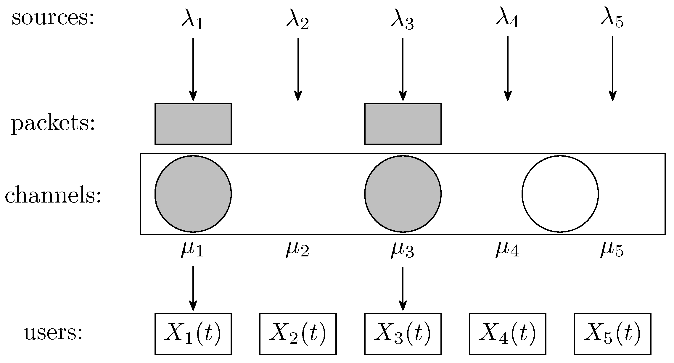
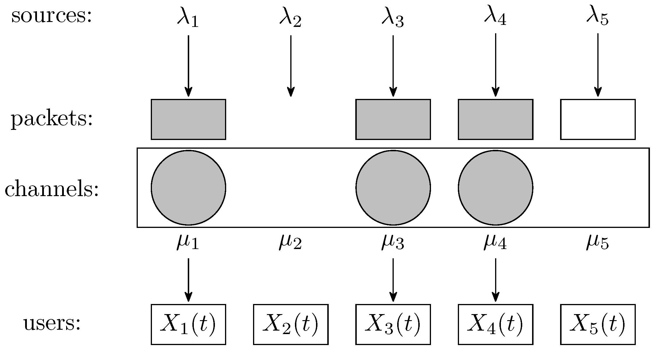
Figure 1 represents a system with channels and users in a slot where two packets from sources 1 and 3 have been generated. Only two channels can be allocated, which is indicated with gray filling. Figure 2 shows a snapshot of the same system with all channels allocated in a slot, as there are at least as many packets available as channels. Yet, the packet from source 5 will be lost, as it cannot be transmitted in the slot.

Figure 1.
System snapshot showing underutilization of channels.
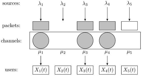
Figure 2.
System snapshot where a generated packet will be lost.
The cost incurred by user n in a slot is given by a general nonnegative and nondecreasing function of its AoI at the beginning of the slot.
At the start of each slot, a controller at the BS decides which packets to attempt to transmit, among those just generated, if any, up to a maximum of M.
We shall assume that action choice is based only on the current joint state. This corresponds to considering scheduling policies from the class of stationary policies that attempt to transmit up to M packets at each slot. We denote by the action chosen for user n in slot t, which can be 1 (attempt transmission of an available packet) or 0 otherwise (note that this action must be taken if no packet is available). As in [14], we shall refer to as the set of controllable states for user n, where both actions are available, and to as the set of uncontrollable states, where only the passive action is available.
The state transition probabilities for user n under action , denoted by for any time slot t, are given by
and, for ,
Given a discount factor , the expected total discounted cost incurred by policy starting from the joint state , where we use the vector notation , , and , is
In (3), is the expectation under policy , conditioned on starting from . The discounted cost problem is to find an admissible policy (i.e., in ) minimizing the cost objective in (3) for any initial joint state .
We shall also consider the average cost problem, which is to find an admissible scheduling policy minimizing the average expected cost per slot, given by
Note that we restrict attention to stationary policies, even though we have not proven that they are optimal among the wider class of history-dependent policies. Conditions ensuring such a result in MDP models with countable states and unbounded costs are given, e.g., in Section 6.10 (discounted criterion) and 8.10 (average criterion) of Puterman [5]. Yet, since such issues are only of ancillary interest to this paper, we do not pursue them here, except for certain single-user subproblems (see Proposition 2).
The above problems are formulated as RMABPs by identifying projects with users and taking the active action on a project with attempting to transmit a packet for a user.
Given the intractability of computing an optimal policy, we aim to design suboptimal policies that can be implemented with low complexity and perform well. Index policies are appealing in this setting; they are based on defining an index for each user n, a scalar function of its controllable states . In a slot starting in , where and are as in (3), the policy attempts to transmit up to M available packets, if any exist, giving higher priority to users with larger nonnegative index values and breaking ties arbitrarily.
This raises the issue of how to design easily computable index policies that perform well, if possible. Regarding ease of calculation, a simple choice is the greedy index policy, based on the index . A more sophisticated idea for constructing index policies was proposed by Whittle [7], as discussed below.
3. Indexability and Whittle Index
This section discusses indexability and the Whittle index, adapting the approach in Whittle [7] to the nuances of the present model. We focus on the discounted cost problem,
where , defined in (3), is the system’s cost metric, giving the expected total -discounted cost under policy starting from . We define to be the optimal cost.
We start by formulating a relaxation of optimization problem (5) by replacing the class of admissible scheduling policies , which can allocate up to K channels per slot, with a larger class of policies. In particular, we use the class of policies , which can allocate up to N channels per slot, and further impose the additional constraint
where and
We shall refer to as the system’s work metric, which gives the expected total discounted number of transmission attempts.
Note that (6) is implied by the sample-path constraints implicit in , namely,
The resulting relaxed problem is
Note that, by construction, the optimal cost of (7) is a lower bound on .
We now attach a nonnegative Lagrange multiplier, or, more properly, since we are dealing with an inequality-constrained optimization problem, a Karush–Kuhn–Tucker (KKT) multiplier, , to constraint (6) in (7), and formulate the Lagrangian function
and the Lagrangian relaxation
Note that multiplier represents a charge per transmission attempt. Again, by construction, the optimal cost of problem (9) gives in turn a lower bound on for any , which follows from the elementary weak duality relation
The Lagrangian dual problem is to find a multiplier yielding the best lower bound:
Note that (11) is a concave optimization problem—since function is concave in , being a minimum of linear functions—which facilitates its computational solution.
We would like to ensure strong duality, meaning that for some satisfying (6) and , and hence, and , where is the optimal value of problem (11). For such a purpose, we adapt the concept of complementary slackness (CS) from inequality-constrained optimization. Given a policy and a multiplier , we say that they satisfy CS if
The next result gives a sufficient condition for strong duality, which can be used to compute the bound .
Proposition 1.
Proof.
The results follow straightforwardly from the above discussion and the identities
□
The solution of the Lagrangian relaxation (9) is further facilitated by the fact that it naturally decouples into the single-user subproblems
for , where denotes the stationary transmission policies for the subsystem corresponding to user n in isolation with a single channel. Note that
and
are the user’s cost metric and work metric, respectively, as defined in Niño-Mora [14]. This follows from considering decoupled policies , where is used on user n, so
hence the Lagrangian function in (8) can be decomposed as
We shall call the model indexable if, for each user n and AoI , there exists a critical transmission attempt charge , which, viewed as an index, characterizes the optimal policies for subproblem (13) under any , as follows: in state , it is optimal—for any initial state —to attempt to transmit if and only if , and it is optimal to not attempt to transmit if and only if . We shall refer to as user n’s Whittle index. Note that we define Whittle’s indexability property as formulated in, e.g., [17,31].
The Whittle index policy for the N-user model gives higher transmission priority to available packets targeted to users with larger nonnegative indices.
4. PCL-Indexability Analysis: Discounted Cost Criterion
This section reviews the PCL-indexability approach in [15,16] and applies it to prove indexability of the single-user subproblems (13) and derive the discounted Whittle index.
4.1. A Verification Theorem for Threshold-Indexability
Consider a single-user subproblem (13), dropping the user label n and writing the AoI cost function as . The discounted cost and work performance metrics are given by
and
so the single-user subproblem of concern is formulated as follows:
We shall write the packet arrival and the transmission success probabilities as and , respectively, dropping the user label. We shall further use the parameter , the probability that in a time slot both a packet is generated and a corresponding transmission attempt succeeds, and consider the complementary probability . Note that , but q may equal 0, in the case of deterministic arrivals and a reliable channel ().
We make the following standing assumption on the one-slot cost function .
Assumption 1.
- (i)
- is nonnegative and nondecreasing;
- (ii)
Note that part (ii) is a mild growth condition on . We next show that Assumption A1 implies the existence of optimal stationary deterministic policies for subproblem (19).
Proposition 2.
Single-user subproblem is solved optimally by stationary deterministic policies determined by Bellman’s equations.
Proof.
The result is trivial in the case . In the case , we apply Theorem 6.10.4 in Puterman [5], which ensures the stated result provided that Assumptions 6.10.1 and 6.10.2 therein hold, which are formulated in terms of an appropriate weight function. Here, we take as the weight function, which satisfies Assumption 6.10.1 in [5] because is bounded under Assumption 1.
To prove Assumption 6.10.2 in [5], we use the sufficient condition provided by Proposition 6.10.5.a in [5]. In the present setting, this reduces to
for some . This follows by verifying that the expression
is decreasing in i, and hence its maximum value is reached by . This allows us to take satisfying (20). □
We shall consider a class of structured policies that intuition suggests might be optimal for problem (19) for any transmission attempt charge , and which will later be proven to be, indeed, optimal: threshold policies, defined as follows. For a nonnegative integer , the k-threshold policy (or k-policy for short) attempts to transmit a packet in controllable state if and only if . We shall write its performance metrics as and .
We shall further consider marginal performance metrics, giving the increments in cost and work metrics under threshold policies resulting from a change in the initial action. Thus, the marginal cost metric for the k-policy starting from is
where denotes the policy that takes action a in the initial time slot and then follows the k-policy from time onward. Note that measures the decrease in cost that results from modifying the k-policy by attempting to transmit initially in state compared to not doing so. The marginal work metric is
which measures the corresponding increase in work expended.
If for every , we further define the marginal productivity (MP) metric
and the MP index
Consider now the following PCL-indexability (PCLI) conditions:
- (PCLI1) Positive marginal work: for every AoI and threshold .
- (PCLI2) Monotone nondecreasing MP index: is nondecreasing in i.
The following verification theorem formulates, in the present setting, a result proven by the author in prior work for restless bandits in increasingly general settings. See [13] [Corollary 2] (finite-state projects), [14] [Theorem 6.3] (finite-state projects with general work metrics), [15] [Theorem 4.1] (semi-Markov countable-state projects), and [17] [Theorem 1 and Proposition 1(c)] (real-state projects). The result refers to threshold-indexability—indexability consistent with threshold policies—meaning that both the model is indexable and threshold policies are optimal for subproblem (19) for any .
Theorem 1.
Suppose that condition (PCLI1) holds. Then, the model is threshold-indexable if and only if condition (PCLI2) holds, with Whittle index given by the MP index, i.e., .
Note that [13,14,15] show that (PCLI1) and (PCLI2) are sufficient conditions for indexability of discrete-state projects, with the Whittle index being given by the MP index. The characterization of threshold indexability in Theorem 1 under (PCLI1) is stated in [17] as a consequence of Theorem 1 and Proposition 1(c) therein.
We emphasize that the PCL-indexability approach does not entail proving first optimality of threshold policies, as in the currently prevailing approach to indexability: both indexability and optimality of threshold policies follow in one fell swoop from Theorem 1.
We next set out to apply Theorem 1 to the present model, which entails verifying PCL-indexability conditions (PCLI1) and (PCLI2).
4.2. Work Metric Analysis and Condition (PCLI1)
We start with condition (PCLI1), namely that the marginal work metric under threshold policies be positive. Recall that the k-policy, with threshold , takes the active action (attempt to transmit) in state if , and the passive action otherwise.
We next address evaluation of the work metric under the k-policy. Even though in the system model we assumed that the AoI i is a positive integer, for obtaining the we include the fictitious value .
From the dynamics in (1) and (2) it follows that the work metric satisfies the following linear equations: for ,
and
In the future, to simplify the notation, we will find it convenient to define
and
The next result gives closed-form expressions for evaluating the work metric .
Lemma 1.
We have
Proof.
See Appendix A. □
The following result evaluates the marginal work metric . Note that we use the standard notation .
Lemma 2.
Proof.
We can use the above results to represent as
□
We thus obtain that the model satisfies condition (PCLI1).
Lemma 3.
, and hence condition (PCLI1) holds.
Proof.
It is immediately apparent from Lemma 2 that is decreasing in i for , and hence
As for , Lemma 2 shows that , which completes the proof. □
4.3. Cost Metric Analysis
We continue by analyzing cost and marginal cost metrics under the k-policy. As above, we will find it convenient to include the fictitious AoI value .
We start by analyzing the cost metric, which satisfies the following linear equations:
and
In the future, to simplify notation, we will find it convenient to define, for ,
We further define quantities as follows. For ,
for ,
and, for ,
The following result gives closed-form expressions for evaluating the cost metric .
Lemma 4.
We have
Proof.
See Appendix B. □
The next result evaluates the marginal cost metric in closed form.
Lemma 5.
We have
- (a)
- (b)
- In particular, in the case ,
Proof.
See Appendix B. □
4.4. MP Index Analysis and Condition (PCLI2)
We next give a closed formula for the discounted MP index defined in (24).
Lemma 6.
We have
Proof.
The result follows straightforwardly from Lemmas 2 and 5, using (30). □
We are now ready to establish the PCL-indexability condition (PCLI2).
Lemma 7.
Under Assumption 1, is monotone nondecreasing, so condition (PCLI2) holds.
Proof.
We have, using that and is nondecreasing,
On the other hand,
Hence, we have, for ,
which completes the proof. □
We thus obtain the following result.
Proposition 3.
Under Assumption 1, the discounted model is threshold-indexable, with Whittle index given by the MP index
Proof.
The result follows from Lemmas 3 and 7 by applying Theorem 1. □
5. PCL-Indexability Analysis: Average Cost Criterion
This section applies Theorem 1 to the present model under the average cost criterion. This entails verifying conditions (PCLI1) and (PCLI2) for average metrics that are counterparts of the discounted metrics above. Note that the PCL-indexability theory under the average criterion, based on Laurent series expansions, is discussed in [13] [Section 5], [14] [Section 6.5], and [15] [Section 5.2], upon which we draw for the following analyses.
5.1. Work Metric Analysis and Condition (PCLI1)
We start with condition (PCLI1), namely the positivity of the marginal work metric under threshold policies. We start by evaluating the average work metric under the k-policy,
The following result evaluates in closed form, which shows that it does not depend on the initial state ; hence, we write it as . This follows from standard results relating discounted and average cost metrics in MDPs. See, e.g., [5] [Theorem 8.10.7]. Note that, below, we incorporate the discount factor in the notation for the discounted metrics considered above to distinguish them from their average criterion counterparts. Thus, e.g., we write the discounted work metric as .
Lemma 8.
We have
Proof.
The result follows by using the expressions for in Lemma 1. □
The next result evaluates the average marginal work metric based on the above formulae for its discounted counterpart, which we now write as .
Lemma 9.
We have
Proof.
The result follows by using the expression for in Lemma 2. □
We thus obtain satisfaction of condition (PCLI1) under the average criterion.
Lemma 10.
, and hence condition (PCLI1) holds.
Proof.
The result follows directly from Lemma 9. □
5.2. Cost Metric Analysis
We continue by analyzing the average cost and marginal cost metrics under the k-policy for , starting with the average cost metric, given by
In the future, we will find it convenient to define (cf. (30)), for ,
Let us now define quantities as follows: for any ,
The following result evaluates in closed form, which shows that it does not depend on the initial state ; hence, we write it as . This follows from standard results (see, e.g., [5] [Theorem 8.10.7]). Below, we denote the discounted cost metric as .
Lemma 11.
We have
Proof.
The result follows by using the formulae for in Lemma 4. □
The next result gives a closed-form expression for the average marginal cost metric , which is the only one needed for our analyses. Below, we denote the discounted marginal cost metric as .
Lemma 12.
We have
Proof.
The result follows by using the expression for in Lemma 5(b). □
5.3. MP Index Analysis and Condition (PCLI2)
We are now ready to address the PCL-indexability condition (PCLI2), namely, the nondecreasingness of the MP index defined by (24), using the marginal metrics for the average cost criterion. The next result gives closed formulae for such an average criterion MP index by drawing on the discounted MP index derived above, which we now denote as .
Lemma 13.
Proof.
The result follows by taking the limit using the formulae in Lemma 6 for . □
We next establish satisfaction of condition (PCLI2).
Lemma 14.
Under Assumption 1, the average criterion MP index is monotone nondecreasing, so (PCLI2) holds.
Proof.
The result follows from the nondecreasingness of the discounted MP index in Lemma 7, since . □
We can now establish the model’s indexability and evaluate its Whittle index.
Proposition 4.
Under Assumption 1, the model is threshold-indexable under the average criterion, with Whittle index given by the MP index
Proof.
The result follows from Lemmas 10 and 13 using Theorem 1 (in its average criterion version). □
6. Index Dependence on Model Parameters and Evaluation for Special Cost Functions
This section exploits the Whittle index formulae obtained above for two interrelated purposes: exploring the dependence of the index on model parameters, drawing corresponding insights, and specializing the index formula to relevant special cost functions.
6.1. Monotonicity of the Whittle Index on the Arrival Rate
We have the following result.
Proposition 5.
Both the discounted Whittle index and the average Whittle index are nonincreasing in the packet arrival probability λ.
Proof.
□
Proposition 5 provides the following insight regarding the packet transmission priority under Whittle’s index policy: other things being equal, the policy gives higher (or, more precisely, not lower) transmission priority to users whose packets arrive at lower rates. This is consistent with the numerical results in [19] [Section 7.1] on the properties of optimal scheduling policies for the special case with reliable channels under the average criterion.
It is readily verified with examples that, for general cost functions, the Whittle index does not need to be monotonic on the transmission success probability . Yet, some monotonicity properties can be identified in the case of special cost functions, as discussed below.
6.2. Whittle Index Formulae for Special Cost Functions
We next consider evaluation of the Whittle index for special cost functions, which yields formulae that can be implemented with greater efficiency than the general formulae above. We shall consider the cases of linear, quadratic, and threshold-type AoI costs.
6.2.1. Linear AoI Cost
We start with the case of a linear cost , with . The discounted index reduces to
and the average criterion index simplifies to
Even though, for general costs, the Whittle index is not necessarily monotonic in the probability of successful transmission , in this special case it turns out to be increasing in (for under the average criterion, since ).
Proposition 6.
For linear costs, the discounted Whittle index is increasing in μ. The same holds for the average Whittle index for .
Proof.
Under the discounted cost criterion, we have
which follows because
Note that (38) holds because increases with i, and the left-most expression in (38) attains the value for and increases with p (recall that ), since
Under the average cost criterion, we have, for ,
This proves the result. □
Hence, for linear AoI costs, other things being equal, Whittle’s policy gives higher transmission priority to users for which packet transmissions are more likely to succeed.
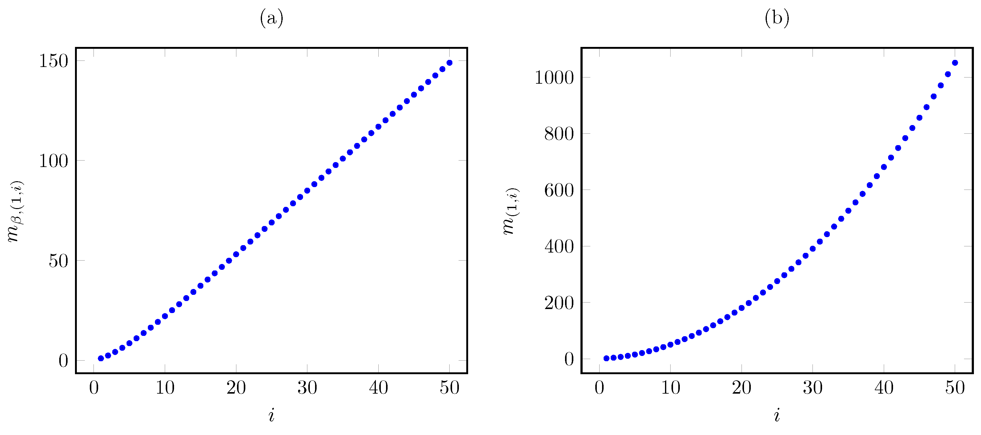
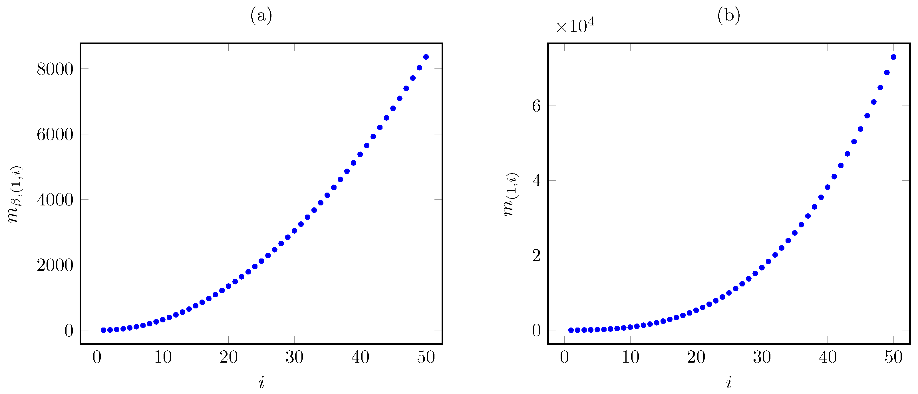
We next graphically illustrate the above results for the base instance with linear cost and the parameters , , and for the states , , and . Figure 3 plots the corresponding Whittle index vs. the AoI under the discounted and average cost criteria. The plots show that the discounted index grows nearly linearly in the AoI, in contrast to the quadratic growth of the average criterion index.

Figure 3.
Discounted (a) and average (b) criterion Whittle index vs. AoI i for linear AoI cost.
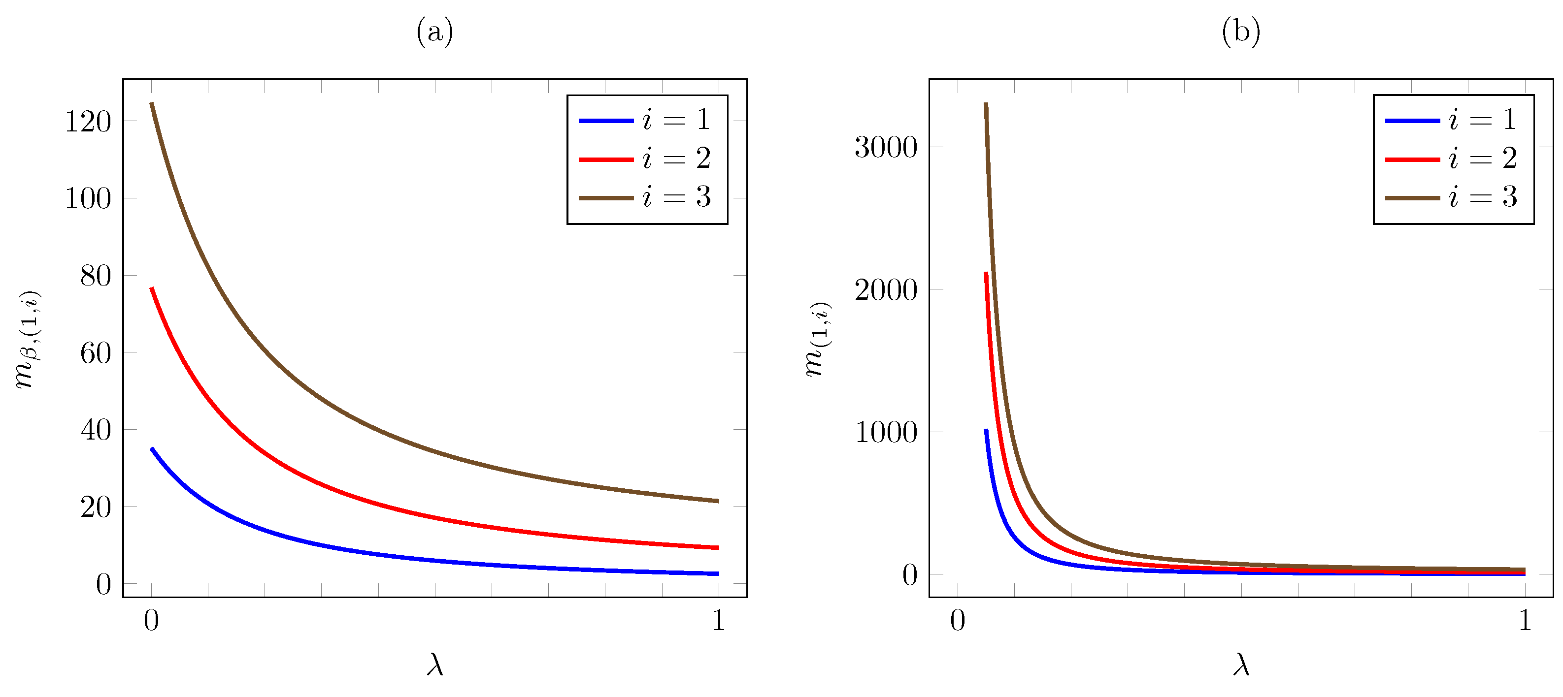
Regarding the dependence on , Figure 4 plots the discounted and the average criterion Whittle indices vs. for AoI values . The plot is consistent with Proposition 5, as the Whittle index is decreasing in . A significant difference is that, as , the discounted index converges to a finite limit, easily seen to be , whereas the average criterion index diverges to infinity. Thus, under the average cost criterion, the increase in priority becomes steeper as the packet arrival probability becomes lower.
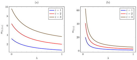
Figure 4.
Discounted (a) and average (b) criterion Whittle index vs. for linear AoI cost.
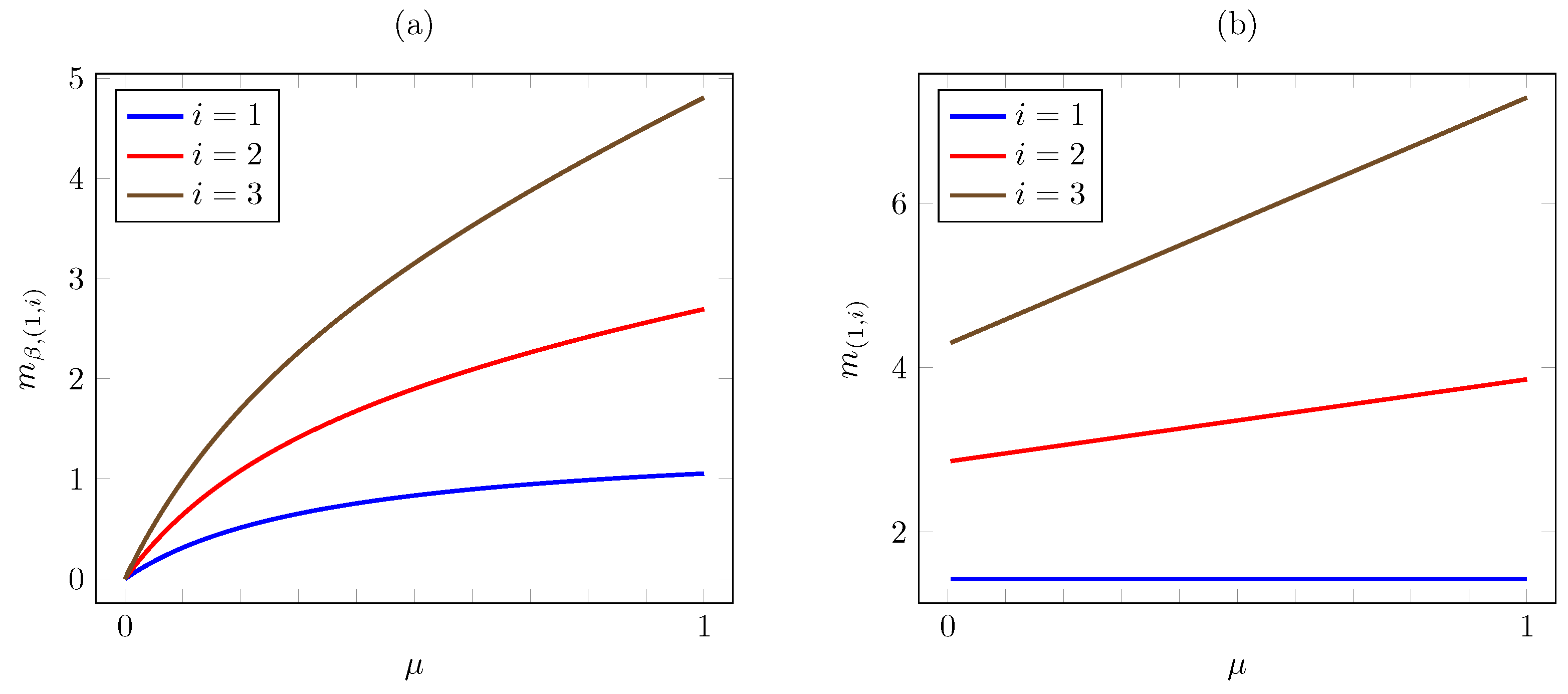
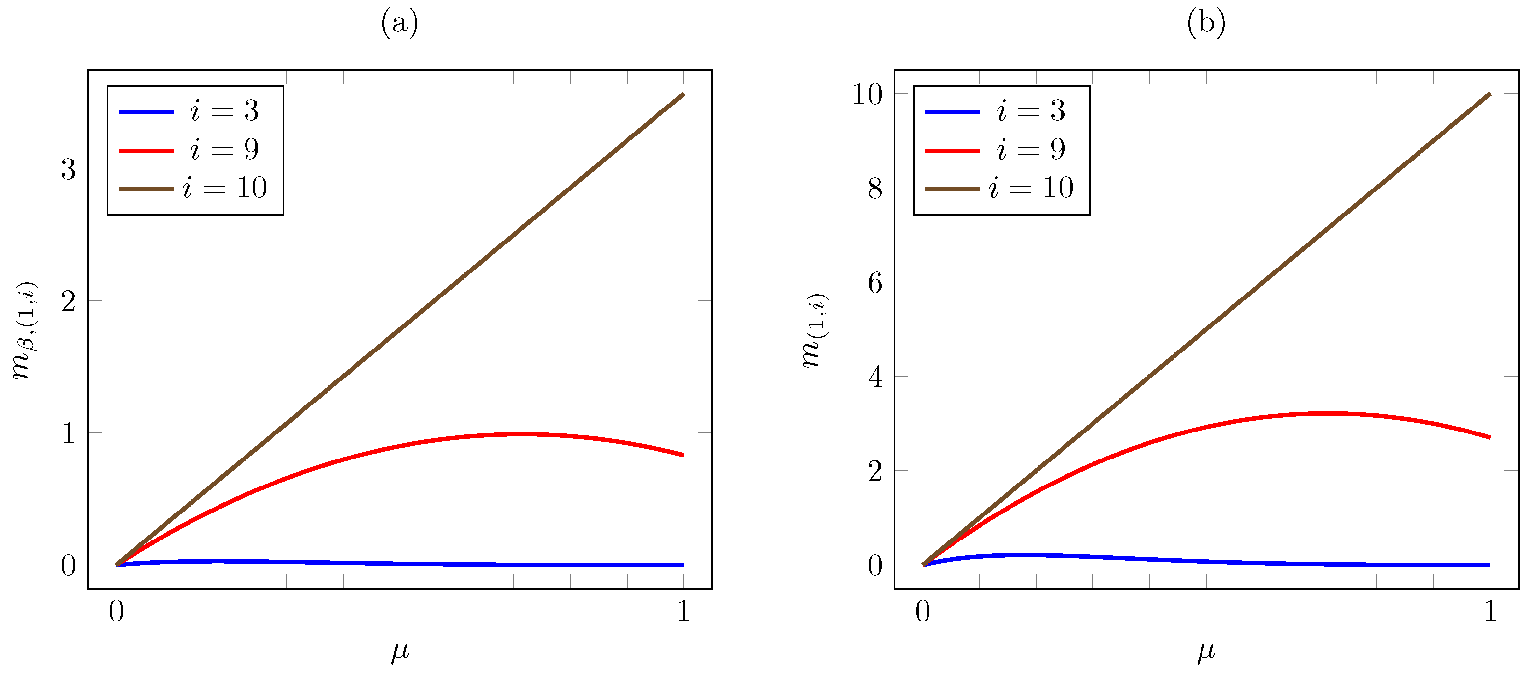
Consider now the dependence on . Figure 5 plots the discounted and the average criterion Whittle indices vs. for AoI values . The plot is consistent with Proposition 6, as the index increases with (except for under the average criterion, where it remains constant as varies). Note that the increase is linear under the average criterion.

Figure 5.
Discounted (a) and average (b) criterion Whittle indices vs. for linear AoI cost.
6.2.2. Quadratic AoI Cost
We next turn to the case of a quadratic cost function . Then, the discounted Whittle index has the evaluation
whereas the average criterion Whittle index reduces to
Considering the same instance as above, Figure 6 plots the corresponding Whittle index vs. the AoI under the discounted and average cost criteria. The plots show that the Whittle index growth with the AoI is much steeper under the average criterion (having cubic growth) than under the discounted criterion (having quadratic growth).
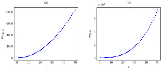
Figure 6.
Discounted (a) and average (b) criterion Whittle index vs. AoI i for quadratic AoI cost.
As for the dependence on , the plots in Figure 7 are also consistent with Proposition 5. As was the case for the linear cost case, we see that, as , the discounted index converges to a finite limit, whereas the average criterion index diverges to infinity.
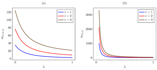
Figure 7.
Discounted (a) and average (b) criterion Whittle indices vs. for quadratic AoI cost.
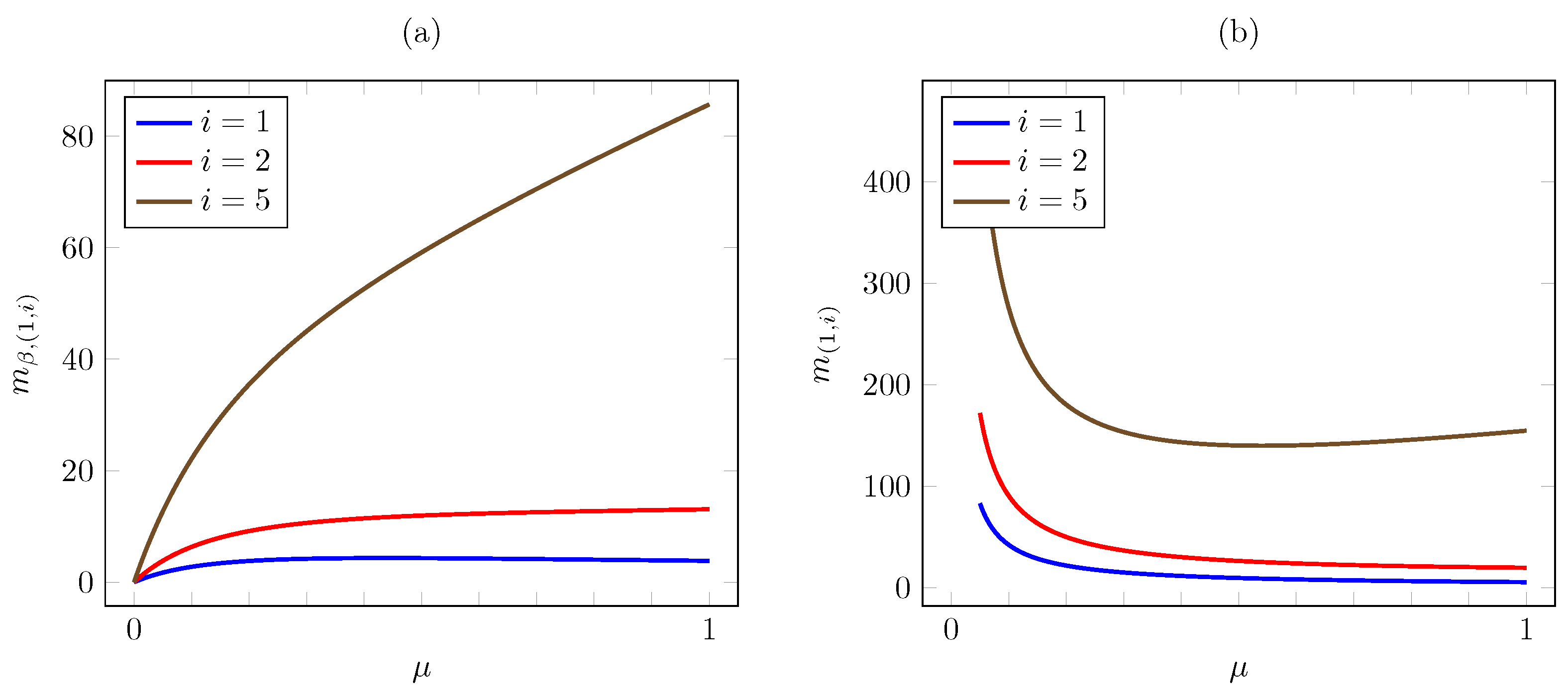
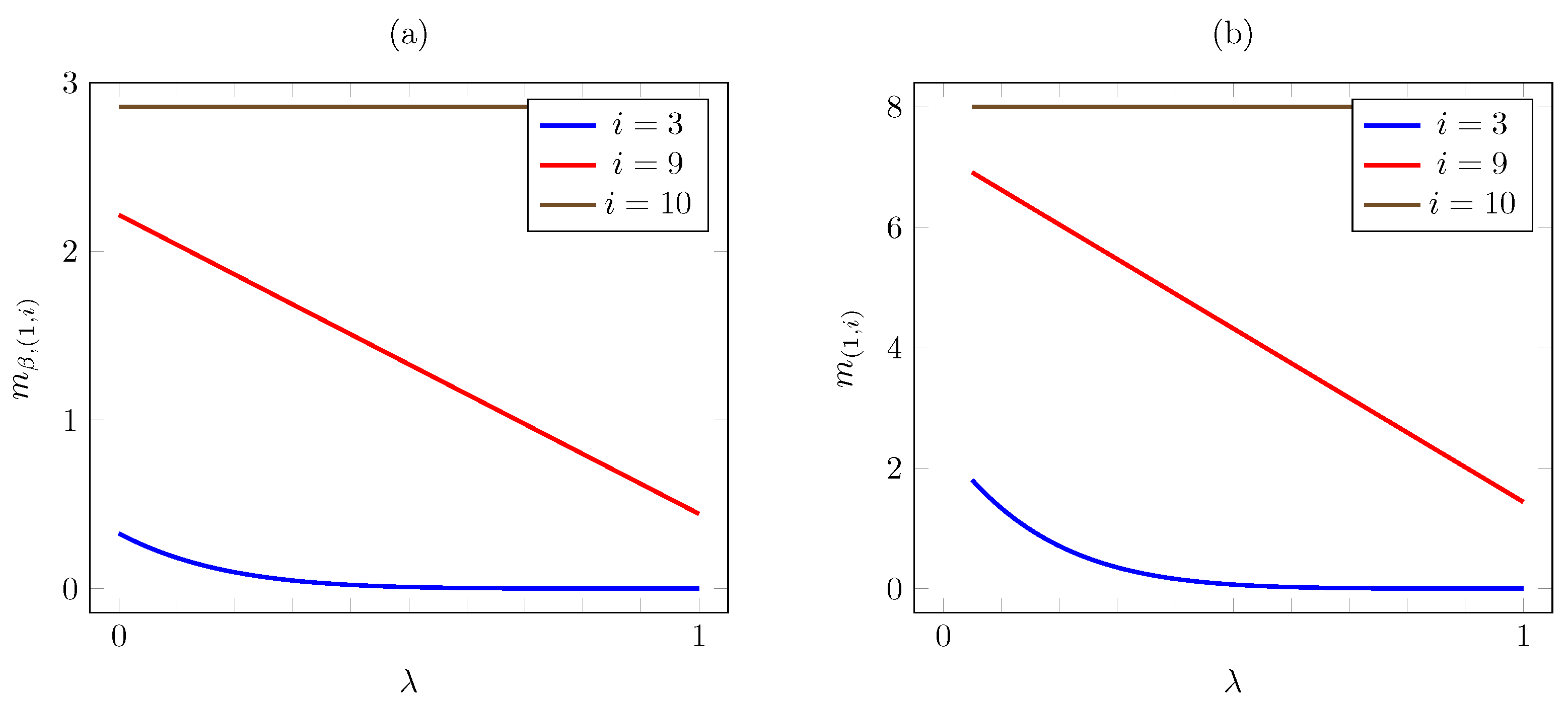
Consider now the dependence on . Figure 8 plots the discounted and the average criterion Whittle index vs. for the same instance. The plot reveals a strikingly different behavior of the discounted and average criterion Whittle indices. Thus, for , the discounted index appears to first increase and then to decrease in . To verify it, note that
and
Thus, for the given instance, we have
and hence increases in for and decreases in for .
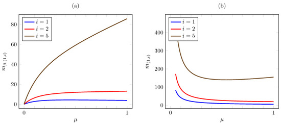
Figure 8.
Discounted (a) and average (b) criterion Whittle indices vs. for quadratic AoI cost.
On the other hand, the plot shows that the discounted Whittle index increases with for and for . It is readily verified analytically that such is the case in this instance for AoI values .
In contrast, the plot shows that the average criterion Whittle index decreases with . We can readily verify this, noting that
and hence
Furthermore, we have, for ,
and hence also decreases with , consistently with the plot.
As for , the plot shows that it first decreases and then increases with . Using (41), it is readily verified analytically that such behavior holds provided , since
and hence has a unique minimum at for such .
The same qualitative behavior holds for where , first decreasing and then increasing with , provided that
since in such cases has a unique minimum as a function of at
Note also that as , , whereas .
6.2.3. Threshold-Type AoI Cost
Finally, consider the case of a threshold-type cost function, with . Then, it is readily verified that the discounted Whittle index is given by
whereas the average criterion index has the evaluation
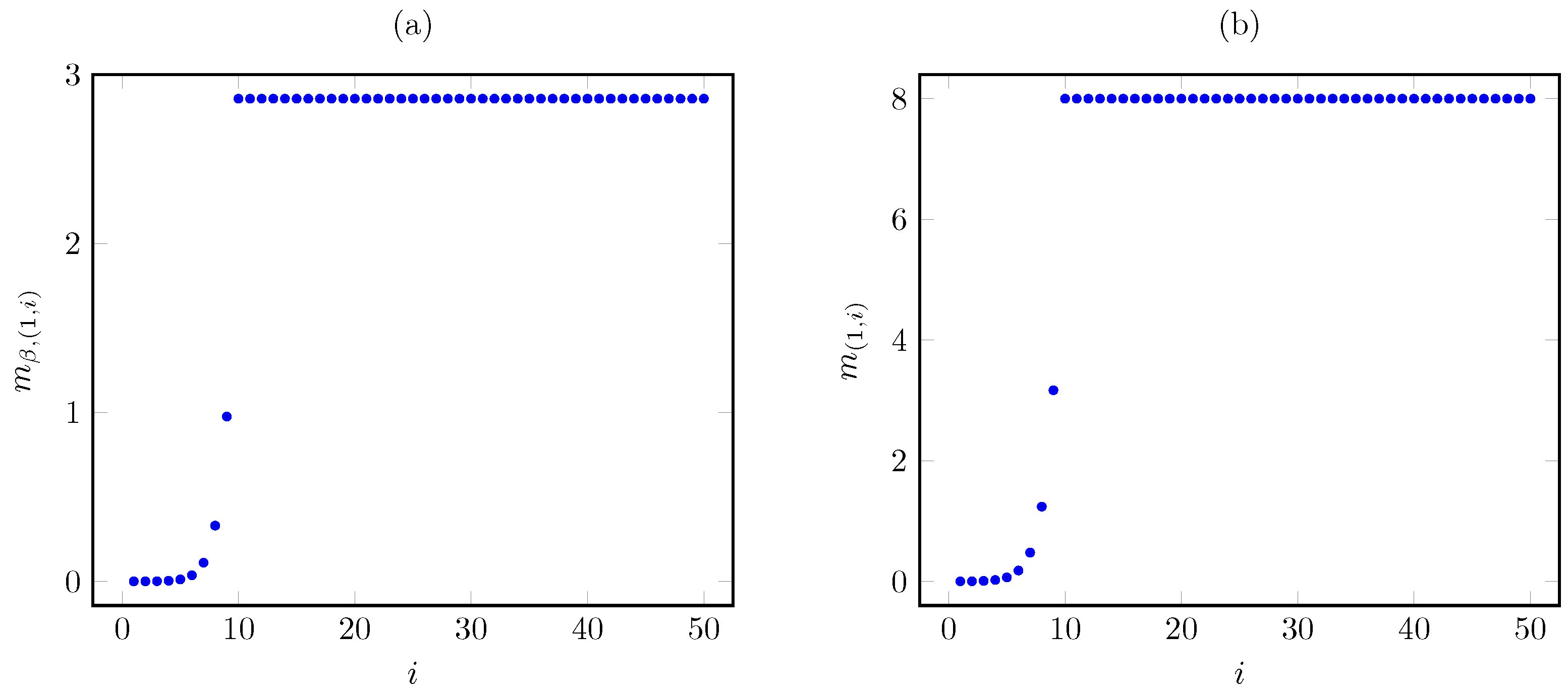
Considering the same instance as above, with , Figure 9 plots the Whittle index vs. the AoI under the discounted and average cost criteria. The plots show that the Whittle index growth with the AoI is slightly steeper for under the average criterion than under the discounted criterion. For , both indices remain constant as the AoI i grows.
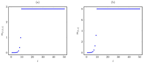
Figure 9.
Discounted (a) and average (b) criterion Whittle index vs. AoI i for threshold-type AoI cost.
Regarding the dependence on , we have
and
Figure 10 plots the discounted and the average criterion Whittle indices vs. . The plot shows that both indices are decreasing in for and remain constant for . Note that the indices decrease linearly with for .
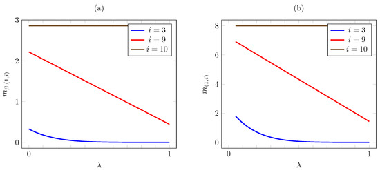
Figure 10.
Discounted (a) and average (b) criterion Whittle indices vs. for threshold-type AoI cost.
As for the dependence of the Whittle index on , we have, for the discounted index,
and, for the average criterion index,
Hence, for , both indices and decrease with whenever , i.e., for , and increase with for sufficiently low values, in particular for . In contrast, for , both indices increase linearly in . Such behavior is illustrated in Figure 11.

Figure 11.
Discounted (a) and average (b) criterion Whittle indices vs. for threshold-type AoI cost.
7. Discussion
This paper has addressed a broad model for scheduling AoI updates simultaneously incorporating the features of random packet arrivals, unreliable channels, and general nondecreasing AoI costs in a no-buffer setting. Indexability (existence of the Whittle index) had only been established in prior work for special cases of this model and only under the average cost criterion using the prevailing approach for indexability analysis, based on first establishing optimality of threshold policies and then exploiting the monotonicity property of the optimal threshold. We have proven that the broad model addressed is indexable and have evaluated its Whittle index in closed form, both under the discounted and the average criterion, by carrying out a PCL-indexability analysis, an approach that has been developed by the author over the last two decades. By demonstrating its effectiveness in a relevant model that had not previously yielded to the prevailing analysis approach, we aim to bring such an approach to the attention of researchers in the area so that they can use it to analyze other models. We have further drawn qualitative insights on how scheduling priority under Whittle’s index policy depends on models parameters by exploiting the closed formulae for Whittle’s index for general costs and for special cost functions. It remains to numerically test the performance of Whittle’s index policy in the present model. Future research directions include carrying out a PCL-indexability analysis in more complex AoI scheduling models, such as those incorporating buffers.
Funding
This research was supported in part by the grant PID2019-109196GB-I00 funded by MCIN/AEI/10.13039/501100011033.
Data Availability Statement
No new data were created or analyzed in this study. Data sharing is not applicable to this article.
Conflicts of Interest
The author declares no conflict of interest. The funders had no role in the design of the study; in the collection, analyses, or interpretation of data; in the writing of the manuscript; or in the decision to publish the results.
Abbreviations
The following abbreviations are used in this manuscript:
| AoI | Age of Information |
| BS | Base station |
| CS | Complementary slackness |
| MABP | Multi-armed bandit problem |
| MDP | Markov decision process |
| MP | Marginal productivity |
| PCL | Partial conservation laws |
| PCLI | PCl-indexability |
| RMABP | Restless multi-armed bandit problem |
Appendix A. Work Metric Evaluation
Proof of Lemma 1.
The fact that can be expressed in terms of the through
follows straightforwardly from (25) and (26).
On the other hand, we have the following recursions for :
Since the recursions in (A2) are readily expressed as a backward and a forward recursion, we need to obtain the value of pivot element to solve them. The following identities readily follow by induction on the first and the second recursions in (A2):
From the first identity in (A3) we obtain . Now, using that as (because ), we obtain
We thus have a linear equation system characterizing and , which yields
From this and (A3) we further obtain for , completing the proof. □
Appendix B. Cost Metric Evaluation
Proof of Lemma 4.
On the other hand, we have the following recursions for :
Since the recursions in (A6) are readily expressed as a backward recursion and a forward recursion, we need to obtain the value of pivot element to solve them. For such a purpose we shall derive equations on and . Thus, from the first recursion we readily obtain by induction the following identities:
To analyze the second recursion in (A6) we need to distinguish two cases, depending on whether or . Consider first the case , in which the second expression in (A6) is not actually a recursion, as it reduces to
Now we solve the linear equation system
to obtain
and
The above expressions give the stated closed-form formulae for in the case .
Consider now the case . Then, the following identities readily follow by induction on the second recursion in (A6): for ,
where we have used that
Now, using that and as (which follows from Assumption 1), we obtain, letting ,
We thus have a linear equation system determining and , which yields
whence
i.e.,
i.e.,
This completes the proof. □
We next give the proof of Lemma 5.
Proof of Lemma 5.
First, we draw on the results in Section 4.3 to represent as
In the case , we have
As for the case , we have (recall that )
This completes the proof. □
References
- Kaul, S.; Gruteser, M.; Rai, V.; Kenney, J. Minimizing age of information in vehicular networks. In Proceedings of the 8th Annual IEEE Communications Society Conference on Sensor, Mesh and Ad Hoc Communications and Networks (SECON), Salt Lake City, UT, USA, 27–30 June 2011; pp. 350–358. [Google Scholar]
- Kaul, S.; Yates, R.; Gruteser, M. Real-time status: How often should one update? In Proceedings of the 31st IEEE International Conference on Computer Communications (INFOCOM), Orlando, FL, USA, 25–30 March 2012; pp. 2731–2735. [Google Scholar]
- Kosta, A.; Pappas, N.; Angelakis, V. Age of information: A new concept, metric, and tool. Found. Trends Netw. 2017, 12, 162–259. [Google Scholar] [CrossRef]
- Yates, R.D.; Sun, Y.; Brown, D.R.; Kaul, S.K.; Modiano, E.; Ulukus, S. Age of information: An introduction and survey. IEEE J. Sel. Areas Commun. 2021, 39, 1183–1210. [Google Scholar] [CrossRef]
- Puterman, M.L. Markov Decision Processes: Discrete Stochastic Dynamic Programming; Wiley: New York, NY, USA, 1994. [Google Scholar]
- Bertsekas, D.P. Dynamic Programming and Optimal Control—Approximate Dynamic Programming, 4th ed.; Athena Scientific: Nashua, NH, USA, 2012; Volume II. [Google Scholar]
- Whittle, P. Restless bandits: Activity allocation in a changing world. J. Appl. Probab. 1988, 25, 287–298. [Google Scholar] [CrossRef]
- Gittins, J.C.; Jones, D.M. A dynamic allocation index for the sequential design of experiments. Colloq. Math. Soc. János Bolyai 1974, 9, 241–266. [Google Scholar]
- Klimov, G.P. Time-sharing service systems. I. Theory Probab. Appl. 1974, 19, 532–551. [Google Scholar] [CrossRef]
- Papadimitriou, C.H.; Tsitsiklis, J.N. The complexity of optimal queuing network control. Math. Oper. Res. 1999, 24, 293–305. [Google Scholar] [CrossRef]
- Weber, R.R.; Weiss, G. On an index policy for restless bandits. J. Appl. Probab. 1990, 27, 637–648. [Google Scholar] [CrossRef]
- Niño-Mora, J. Markovian restless bandits and index policies: A review. Mathematics 2023, 11, 1639. [Google Scholar] [CrossRef]
- Niño-Mora, J. Restless bandits, partial conservation laws and indexability. Adv. Appl. Probab. 2001, 33, 76–98. [Google Scholar] [CrossRef]
- Niño-Mora, J. Dynamic allocation indices for restless projects and queueing admission control: A polyhedral approach. Math. Program. 2002, 93, 361–413. [Google Scholar] [CrossRef]
- Niño-Mora, J. Restless bandit marginal productivity indices, diminishing returns and optimal control of make-to-order/make-to-stock M/G/1 queues. Math. Oper. Res. 2006, 31, 50–84. [Google Scholar] [CrossRef]
- Niño-Mora, J. Dynamic priority allocation via restless bandit marginal productivity indices (with discussion). TOP 2007, 15, 161–198. [Google Scholar] [CrossRef]
- Niño-Mora, J. A verification theorem for threshold-indexability of real-state discounted restless bandits. Math. Oper. Res. 2020, 45, 465–496. [Google Scholar] [CrossRef]
- Kadota, I.; Sinha, A.; Uysal-Biyikoglu, E.; Singh, R.; Modiano, E. Scheduling policies for minimizing age of information in broadcast wireless networks. IEEE/ACM Trans. Netw. 2018, 26, 2637–2650. [Google Scholar] [CrossRef]
- Hsu, Y.P.; Modiano, E.; Duan, L.J. Scheduling algorithms for minimizing age of information in wireless broadcast networks with random arrivals. IEEE Trans. Mobile Comput. 2020, 19, 2903–2915. [Google Scholar] [CrossRef]
- Sun, Y.; Uysal-Biyikoglu, E.; Yates, R.D.; Koksal, C.E.; Shroff, N.B. Update or wait: How to keep your data fresh. IEEE Trans. Inform. Theory 2017, 63, 7492–7508. [Google Scholar] [CrossRef]
- Jhunjhunwala, P.R.; Moharir, S. Age-of-information aware scheduling. In Proceedings of the IEEE International Conference on Signal Processing and Communications (SPCOM), Bangalore, India, 10–16 April 2018; pp. 222–226. [Google Scholar]
- Tripathi, V.; Modiano, E. A Whittle index approach to minimizing functions of age of information. In Proceedings of the 57th Annual Allerton Conference on Communication, Control, and Computing, Monticello, IL, USA, 24–27 September 2019; pp. 1160–1167. [Google Scholar]
- Maatouk, A.; Kriouile, S.; Assaad, M.; Ephremides, A. On the optimality of the Whittle’s index policy for minimizing the age of information. IEEE Trans. Wirel. Commun. 2021, 20, 1263–12770. [Google Scholar] [CrossRef]
- Kriouile, S.; Assaad, M.; Maatouk, A. On the global optimality of Whittle’s index policy for minimizing the age of information. IEEE Trans. Inf. Theory 2022, 68, 572–600. [Google Scholar] [CrossRef]
- Sun, J.Z.; Jiang, Z.Y.; Krishnamachari, B.; Zhou, S.; Niu, Z.S. Closed-form Whittle’s index-enabled random access for timely status update. IEEE Trans. Commun. 2020, 68, 1538–1551. [Google Scholar] [CrossRef]
- Sun, J.Z.; Jiang, Z.Y.; Zhou, S.; Niu, Z.S. Optimizing information freshness in broadcast network with unreliable links and random arrivals: An approximate index policy. In Proceedings of the 38th IEEE International Conference on Computer Communications Workshops (INFOCOM WKSHPS), Paris, France, 29 April–2 May 2019; pp. 115–120. [Google Scholar]
- Tang, Z.F.; Sun, Z.; Yang, N.; Zhou, X.Y. Whittle index-based scheduling policy for minimizing the cost of age of information. IEEE Commun. Lett. 2022, 26, 54–58. [Google Scholar] [CrossRef]
- Badia, L.; Munari, A. Discounted age of information for networks of constrained devices. In Proceedings of the 20th Mediterranean Communication and Computer Networking Conference (MedComNet), Pafos, Cyprus, 1–3 June 2022; pp. 43–46. [Google Scholar] [CrossRef]
- Wu, T.; Wen, P.; Tang, S.D. Optimal scheduling strategy of AUV based on importance and age of information. Wirel. Netw. 2023, 29, 87–95. [Google Scholar] [CrossRef]
- Zhang, M.; Arafa, A.; Huang, J.; Poor, H.V. Pricing fresh data. IEEE J. Sel. Areas Commun. 2021, 39, 1211–1225. [Google Scholar] [CrossRef]
- Niño-Mora, J. A dynamic page-refresh index policy for web crawlers. In Proceedings of the 21st International Conference on Analytical and Stochastic Modelling Techniques and Applications (ASMTA), Budapest, Hungary, 30 June–2 July 2014; Sericola, B., Telek, M., Horváth, G., Eds.; Lecture Notes in Computer Science. Springer: Berlin/Heidelberg, Germany, 2014; Volume 8499, pp. 46–60. [Google Scholar]
Disclaimer/Publisher’s Note: The statements, opinions and data contained in all publications are solely those of the individual author(s) and contributor(s) and not of MDPI and/or the editor(s). MDPI and/or the editor(s) disclaim responsibility for any injury to people or property resulting from any ideas, methods, instructions or products referred to in the content. |
© 2023 by the author. Licensee MDPI, Basel, Switzerland. This article is an open access article distributed under the terms and conditions of the Creative Commons Attribution (CC BY) license (https://creativecommons.org/licenses/by/4.0/).

