Abstract
Polar codes, as the coding scheme for the control channel in fifth-generation mobile communication technology (5G), have attracted widespread attention since their proposal. As a mainstream decoding algorithm for polar codes, the successive cancellation list (SCL) decoder usually improves the error correction performance by increasing the list size, but this method suffers from the problems of high decoding complexity. To address this problem, this paper proposes a layered-search bit-flipping (LS-SCLF) decoding algorithm based on SCL decoding. Firstly, a new flip-bit metric is proposed, which derives a formula to approximate the probability of an error occurring in an information bit. This formula introduces a perturbation parameter to improve the calculation accuracy. Secondly, a compromise scheme for determining the perturbation parameter is proposed. The scheme uses Monte Carlo simulation to determine an optimized parameter for the precise positioning of the first erroneous decoded bit under different decoding conditions. Finally, a layered search strategy is adopted to sequentially search the erroneous decoded bits from the low order to high order, which can correct up to multiple bits at the same time. Simulation results show that the proposed algorithm achieves improved error correction performance with a slight increase in decoding complexity compared to the generalized SCL-Flip (GSCLF) decoding algorithm. This algorithm also achieves a good balance between the error correction performance and decoding complexity.
MSC:
94B35
1. Introduction
Polar codes are the first channel coding scheme that can be rigorously proven to achieve channel capacity [1], with clear construction methods and low-complexity encoding and decoding algorithms compared to LDPC codes [2] and turbo codes [3]. Therefore, polar codes have been regarded as an important innovation in channel coding in recent years and have great theoretical value and application potential in future wireless communications, thus attracting much attention from researchers. In 2016, polar codes have been identified as the control channel coding scheme for the fifth-generation enhanced mobile broadband (eMBB) scenario, marking the leap from theoretical research to practical application. Meanwhile, after more than a decade of development, polar codes have achieved many research achievements in deep space communications [4,5], underwater acoustic communications [6,7,8], optical communications [9,10,11,12], and so on.
Although polar codes have many advantages, they still face challenges in practice. In particular, the error correction performance of polar codes for short and moderate lengths under successive cancellation (SC) decoding is unsatisfactory due to insufficient channel polarization. To break the bottleneck of SC decoding performance, successive cancellation list (SCL) decoding [13] was proposed, which greatly improved the error correction performance at finite lengths by retaining L (L is denoted as list size) decoding paths at each information bit. Subsequently, cyclic redundancy check (CRC)-aided SCL (CA-SCL) decoding [14] further improved the error correction performance by concatenating a CRC code at the end of the polar code to assist in making the final output among the L candidate decoding paths. In early SCL decoding, increasing L was the most direct way to improve the error correction performance. However, as L increases, this method faces two problems: (1) If L is too large, the error correction performance gain becomes very small and diminishes as L continues to increase. (2) It requires more hardware resources and more decoding overhead. For this reason, many decoding algorithms have been studied in terms of adaptive lists [15], path-splitting strategies [16,17,18], and fast decoding [19,20,21] to compensate for the increase in decoding complexity. However, these decoders do not address the problem of improving the error correction performance of CA-SCL decoding with a limited list size.
Inspired by the bit-flipping algorithms [22,23,24,25,26,27] based on SC decoding, the idea of bit-flipping was introduced in SCL decoding. The reference [28] first proposed a successive cancellation list bit-flipping (SCLF) decoding algorithm. This decoding algorithm improves the critical set in [25] to identify the candidate flip-bit and flips one bit in each extra decoding. Experimental results show that the SCLF decoding has better error correction performance than SCL decoding in the medium to high SNR regions. However, the bit-flipping strategy used in this algorithm may lead to the appearance of two identical candidate paths, interfering with the final decoding choice. Reference [29] proposed a shift-pruning decoding algorithm, the essence of which is also to correct the erroneous decoded bits by extra decoding. This algorithm can better balance the error correction performance and decoding complexity, but it lacks flexibility in determining the shift positions of the flip-bit, which leads to its poor applicability. Reference [30] also proposed a bit-flipping-based SCL (BF-SCL) decoder, which developed a new criterion for determining the flipping priority of information bits and a specific bit-flipping strategy. However, the proposed bit-flipping metric only considers the effect of information bits on erroneous decoding, which limits the improvement in error correction performance and also introduces a perturbation parameter that varies with the decoding conditions, causing complex complexity. Reference [31] proposes the generalized SCL-Flip (GSCLF) decoding algorithm, which uses the path metrics of the reserved and eliminated paths to devise a new method for determining the flipping priority of information bits that can quickly locate the erroneous decoded bits. Compared to the decoding algorithms proposed in [28,29,30], the GSCLF decoding is able to correct up to erroneous decoded bits caused by channel noise at the same time, thus providing better error correction performance while maintaining a low decoding complexity. These decoding algorithms improve the error correction performance with a limited list size by correcting the erroneous decoded bits in extra decoding attempts. They can achieve the same or better error correction performance as SCL decoders with larger list sizes.
The flip-bit metric is essential for determining the flipping priority of the information bits, which directly affects the error correction performance and the decoding complexity. In this paper, we draw on the metric proposed in D-SCFlip decoding [27] to design a new flip-bit metric to approximate the probability of the erroneous decision occurance on an information bit. The metric introduces a perturbation parameter that is optimized by simulations to improve the calculation accuracy. Unlike other methods, this metric reflects the sequential nature of SCL decoding, and the metrics between the forward and backward information bits are closely correlated, allowing good localization of erroneous decoded bits. Based on this metric, we propose the layered-search bit-flipping (LS-SCLF) decoder, which searches for erroneous decoded bits sequentially from low order to high order and can correct up to bits in one extra decoding attempt. Simulation results show that the proposed decoding algorithm can achieve a good balance between error correction performance and decoding complexity.
The remainder of the paper is organized as follows. Section 2 introduces the polar codes, SCL decoder, CA-SCL decoder, and SCL-Flip decoder. Section 3 details the proposed flip-bit metric and the the LS-SCLF decoding algorithm. Simulation results are provided in Section 4, and the conclusions are drawn in Section 5.
2. Preliminaries
2.1. Polar Codes
In this paper, denotes the vector . We denote by the polar code, where N is the code length and K is the length of information bits. It should be noted that if a CRC code is concatenated at the end of a polar code to improve the error detection capability of the polar code, then , where k is the number of information bits of the CRC code and r is the number of check bits of the CRC code. The rate is denoted by R and is calculated as .
Since N independent and identically distributed binary symmetric channels can form N sub-channels with different channel capacities after polarization, we select the first K sub-channels with the largest channel capacity to transmit information bits and denote the index set of these reliable sub-channels by . The remaining subchannels are used to transmit frozen bits, which are usually set to 0 and known by both the transmitter and receiver. The index set of frozen bits is denoted as .
The encoding of polar codes is expressed as:
where denotes the data vector, and it consists of K information bits and frozen bits. denotes the encoded vector and denotes the generator matrix. For any information bit , , when successive cancellation decoding is used, its hard decision estimation can be expressed as:
where is the LLR of , and it can be computed as:
where and denote the probabilities of and under the condition , respectively. denotes the received vector of the receiver.
2.2. SCL Decoder and CA-SCL Decoder
The framework of the SCL (CA-SCL) decoder is shown in Figure 1. Firstly, to improve the error correction performance of SC decoding, the SCL decoder retains both sub-paths after the path splitting at any information bit to increase the probability that the correct path is obtained in the candidate paths. Secondly, if the number of candidate paths reaches , they are ranked in ascending order by the path metric, and the L paths with the smallest metric are reserved through path competition. Finally, the SCL decoder selects the path with the smallest metric as the decoding result at the end of decoding. CA-SCL decoding is almost the same as SCL decoding, and the only difference is that CA-SCL decoding selects the path that passes the CRC check as the decoding output.
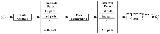
Figure 1.
Framework of the SCL (CA-SCL) decoder.
2.3. SCL-Flip Decoder
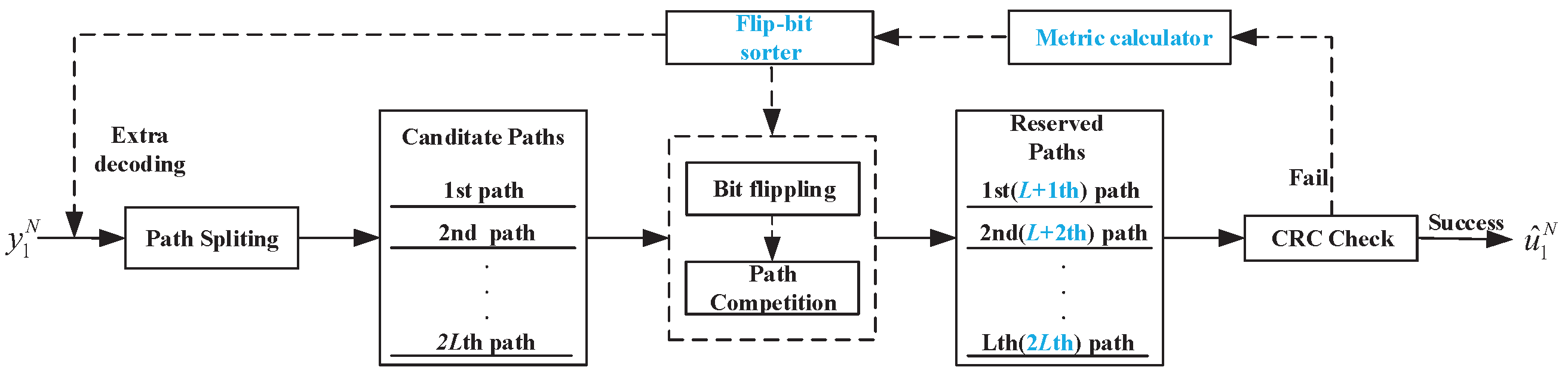
The SCL-Flip decoder originates from the CA-SCL decoder, with the difference that when the CA-SCL decoder fails the CRC check, the SCL-Flip decoder performs extra decoding attempts to correct the suspiciously erroneous decoded bits, and its framework is shown in Figure 2. The extra decoding procedures for the SCL-Flip decoder are as follows. Firstly, if the CA-SCL decoding (initial SCL decoding) fails the CRC check, the metric calculator calculates the flip-bit metric, and the flip-bit sorter sorts and selects the candidate flip-bit based on their metrics. Secondly, the SCL-Flip decoding performs extra decoding and adds bit-flipping to the path competition. In other words, it makes the opposite decision to CA-SCL decoding for the element in the candidate flip-bit; i.e., it keeps the L decoded paths with the largest path metric (the th to th paths of the candidate paths) while decoding the other bits as CA-SCL decoding. If the extra decoding fails the CRC check, the above operation continues until the decoding is successful or the maximum number of extra decoding attempts is reached.

Figure 2.
Framework of the SCL-Flip decoder.
In particular, for a better interpretation of the SCL-Flip decoding, we denote as a flip-bit set of any order , where , , , , and is the index set of the first information bits. Without loss of generality, is denoted as the decoding of by SCL-Flip decoder, and is denoted as that has finished decoding the first elements and to decode the tth element, obviously, . In the remainder of this paper, SCLF(0) is denoted as the initial SCL decoding. To clearly indicate the decoding step and distinguish each decoding path, for , and respectively denote the reserved paths list and eliminated paths list of at the step that decoding , where stands for the lth decoding path and stands for the decoding path with . For ease of presentation, let be denoted as both paths simultaneously. For , decodes the same way as SCLF(0). Similarly, and correspond to the reserved paths list and eliminated paths list of SCLF(0) when decoding , respectively. Specifically, for , and .
In addition, we denote as the PM of . For , let and the corresponding is denoted as . Obviously, is the sub-vector of and it consists of the first k elements in . For , , . For , both and are null vectors. can be computed as:
where is the LLR of and can be obtained by:
Assume that is the trajectory that all its elements are indexes of the erroneous decoded bits caused by channel noise. When the decoding is executed to (), candidate paths are obtained through path splitting, and these candidate paths are sorted by their metrics to satisfy . After path competition, we can obtain the reserved paths list; i.e., . Based on the definition of SCL-Flip decoding, and satisfy the following relationship:
In particular, for a trajectory of order 1, the above relationship can be written as:
3. The LS-SCLF Decoder
3.1. Framework of the LS-SCLF- Decoder
Channel noise and error propagation are the two causes of erroneous decoding decisions in SCL decoding. In particular, the first erroneous decoded bit is entirely caused by the channel noise so that the error propagation does not affect the word-error rate (WER) performance. In practice, especially under low signal-to-noise ratio (SNR) conditions, there are often several erroneous decoding decisions that are caused by channel noise. Therefore, the bit-flipping algorithm for the correction of the first erroneous decision alone does not solve the case of multiple erroneous decoded bits caused by channel noise.
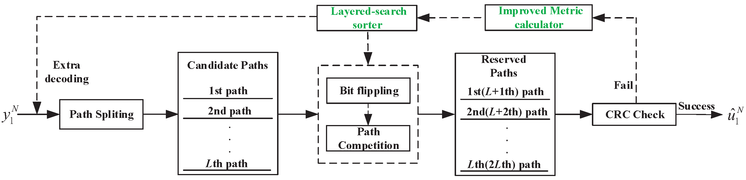
Based on the above analysis, this paper proposes the layered-search SCL-Flip decoder that can correct up to erroneous decoded bits simultaneously, i.e., the LS-SCLF- decoder. The framework of LS-SCLF- is shown in Figure 3, which is almost the same as the SCL-Flip decoder, it but has features in terms of the flip-bit metric and the bit-flipping strategy.

Figure 3.
Framework of the decoder.
3.2. The Proposed Flip-Bit Metric
For SCLF(0), we define the first erroneous decision occurring at information bit () as event , i.e., , . Let denote the probability of , then the mathematical definition of can be expressed as:
For , since there is no path competition, . The calculation of is an arduous task, due to the fact that all the previous bits must be correctly decoded. To simplify the calculation, we approximate it with the following equation:
One can calculate by taking the definition of [32]:
Based on (15), [30] derives the following equation:
In [30], (16) is carried directly into (14), and a perturbation parameter is introduced to calculate the flip-bit metric to determine the priority of the flip-bit. However, the method only considers the effect of information bits and ignores the role of frozen bits for the erroneous decoded bits. To solve this problem, this paper proposes a new metric. Let () be denoted as the ratio that is the sum of the probability of the reserved paths to that of the eliminated ones for and referred to as Probability Ratio (PB), i.e.,
and a higher value of indicates a higher probability of , while a smaller value of indicates a higher probability of . Since the decoding paths in can be treated as the input to the next bit in the SCLF(0) decoding, the PB of the previously decoded bits affects the result of the following bits if the L decoding paths are considered as a whole. Therefore, PB is to SCLF(0) decoding what LLR is to SC decoding.
For a flip-bit , the probability that is the erroneous decoded path is denoted as . Referring to (12)–(13) in [27], can be computed as:
where
By simple calculation, the above equation can be unfolded to the following expression:
Note that the second product of the right-hand side term of (20) is taken only over indexes , since for . In addition, the calculation of is also a complex task. This paper draws on (14) in [27] and proposes a formula to approximate it:
where is the perturbation parameter and , denotes the value of in the logarithmic domain; i.e., . Such a perturbation directly affects the results of (21). In practice, can be optimized by Monte Carlo simulation. On the basis of (20) and (21), the proposed metric associated with flip-bit is defined as:
It is clear that for set , consisting of the first elements of , the following relationship is satisfied between its metric and :
Equation (23) shows that can be regarded as part of , which fully reflects the sequential nature of SCL decoding. In particular, for a one-order flip-bit , the above metric can be rewritten as:
Based on the fact that , (22) can be further rewritten as:
To improve the numerical stability, by taking the logarithm of (22), i.e., , we obtain the equivalent logarithmic domain metric:
Based on the above considerations, the priority of a flip-bit should be in descending order of or ascending order of . In other words, the higher the value of (or the smaller the value of ), the higher the flipping priority of the corresponding flip-bit. For convenience, the remainder of this paper will use as the path metric.
3.3. Optimization of the Perturbation Parameter
The parameter is a key factor for calculating the flip-bit metric. This subsection investigates the optimization of to give higher flipping priority to the channel-induced erroneous decoded bits, thus achieving the goal of correcting the erroneous decoding with a minimum number of additional decoding attempts. In contrast to the D-SCFlip decoding [27], the factors that affect the in the proposed decoding are not only N, R, and SNR but also L. Therefore, the complexity of optimizing the perturbation parameter should be very high, and it cannot even find a global optimal parameter. To improve the practicality, this paper proposes a compromise method of optimizing the perturbation parameter for the first erroneous decoded bit only.
We denote by () the index where the first erroneous decision occurs in the initial SCL decoding, and the corresponding information bit is denoted as . Let denote the list of all the one-order flip-bit, ordered according to decreasing values of their metrics. We denote by the rank of within . The smaller the value of , the higher the flipping priority of the information bit , and thus we denote by the optimized perturbation parameter and define it as:
where denotes the expected value of random variable . Since it is very difficult to solve directly, we will investigate the law between the expected value of and for different decoding conditions to obtain indirectly. The main ideas are as follows. Firstly, let denote the expectation value of for a given decoding condition and investigate the relationship between and under different conditions of N, R, SNR, and L separately. Secondly, we analyze and summarize the laws reflected in the above relationships. Finally, the data fitting and other methods are used to derive the .
To investigate the relationship between and under different conditions, we take the relationship between and under various SNR values as an example, and the process is as follows:
- Fix parameters N, R, and L, and set the value of SNR.
- Set the range and step size of , and the number of Monte Carlo simulations.
- Perform the Monte Carlo simulation for the current and SNR values. If the initial SCL decoding does not pass the CRC check, first construct the list , then find the rank of and note it as . Finally, calculate the average value of after all experiments are completed and denoted as .
- Update the value and return to step (3). Continue to calculate for the new value until the traversal of is complete. Plot the relationship between and , then derive the relationship between the two at that SNR value.
- Update the SNR values and complete steps (1)–(4) again to obtain the relationship between the and for different SNR values.
Specifically, in this paper, to obtain the relationship between and where is the variable, we first set the dB and the fixed parameters , , , (theoretically , but in our experiments we set the range according to the specific situation as ); the step size is 0.2, and the number of Monte Carlo simulations is . Second, independent CA-SCL decoding experiments are performed for at and dB according to step (3), and the corresponding value is obtained. Then, according to step (4), the value of is updated according to the step size and returned to step (3) to obtain a new value, and so on; when the traversal of is completed, the relationship curve between and at dB can be obtained. Finally, according to step (5), the value is sequentially updated and the above experiment is repeated to obtain the relationship between and under various values.
Following the above steps, we can also obtain the relationship between and when L, N, and R are the variables, respectively. For L as the variable, we set ; the fixed parameters , , dB; and the . For N as the variable, we set ; the fixed parameters , , dBl; and the . Similarly, for R as the variable, we set ; the fixed parameters , , dB; and .
3.4. The Detailed Description of the Proposed Decoding Algorithm
For ease of presentation, we denote as the flip-bit list, in which every element is of order l(), and is the number of elements in . For , it contains l elements and ordered in ascending order. is denoted as the metric list corresponding to . For , is the metric of where .
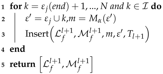
The detailed algorithm of LS-SCLF- decoding is described in Algorithm 1, and the main decoding procedure is as follows: if the initial SCL decoding fails, the and are initialized by the function , and the bit-flipping is performed by for the elements in one by one. Whenever incorrect decoding occurs, the and are updated by the function based on the current flip-bit. Once a successful decoding occurs, the decoding ends, and the final path is output. If and only if all the extra decoding attempts for the one-order flip-bit fail the CRC check, the decoder proceeds to the next round of additional decoding and follows the above process until a successful decoding occurs or the maximum number of extra decoding is reached. The following is the specific description about the key functions in LS-SCLF- decoding:
| Algorithm 1: LS-SCLF- Decoder. |
 |
- (): The initialization strategy is detailed in Algorithm 2. The preliminary flip-bit list is constructed as , and (24) gives the calculation of . Then, the elements in are sorted in descending order by the function, with the largest elements constructing and the corresponding indexes constructing .
- : is the jth element in , i.e., . The function flips all the information bits corresponding to the in turn in an extra decoding attempt.
- : The update algorithm is detailed in Algorithm 3. If fails to pass the CRC check and ; it first calculates the of by (25), where , , and represents the last element of . Then, the function inserts and into the appropriate positions in and , respectively, according to the value of . If the number of elements in exceeds , then only the first elements of and are retained. Since , will be inserted into a position behind .
| Algorithm 2: . |
1 2 3 return |
| Algorithm 3: . |
 |
4. Experiment Design and Simulation Analysis
In this section, two experiments are conducted to verify the performance of the LS-SCLF- decoder. The first experiment is to optimize the perturbation parameter. We use Monte Carlo simulation to derive the relationships between and N, R, L, and SNR and then summarize the applicable range or a certain value under the decoding conditions in this paper. Based on the conclusion of the first experiment, the second experiment simulates the LS-SCLF- decoding and compares it with related decoding methods in terms of error correction performance and complexity to verify the advantages and disadvantages of the proposed algorithm. It should be noted that all experiments in this paper are carried out under the binary-input additive white Gaussian noise channel, and the information bits are selected using the Gaussian approximation algorithm for specific SNR values.
4.1. Perturbation Parameter Optimization
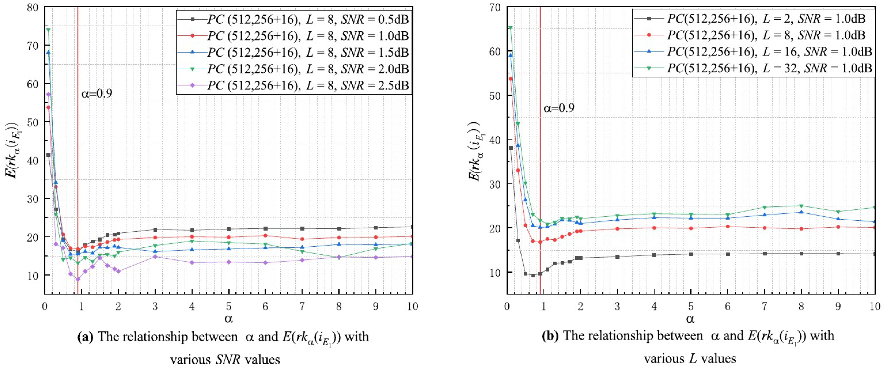
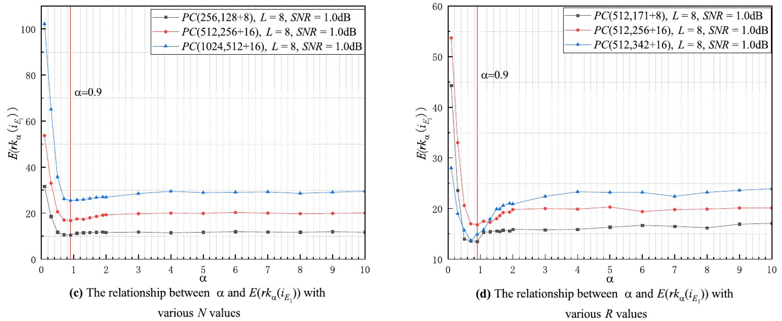
In this subsection, the experiments on the relationship between and are carried out under different , L, N, and R conditions according to the strategy given in Section 3.3 and the relationship curves are shown in Figure 4a–d, respectively. In Figure 4a, all of the curves gradually decrease as increases, and they reach their minimum value at around , after which the curves stabilize. This suggests that the minimum value of is not impacted by the values of , and that the first erroneous decoded bit has the highest flipping priority at under any condition. In Figure 4b, all the curves decrease with increasing and reach a minimum value around , and they gradually converge as continues to increase. This indicates that the minimum value of is also not affected by the value of L, and the first erroneous decoded bit obtains the highest flipping priority around with any L. Moreover, the curves in Figure 4c,d have approximately the same trend as those in Figure 4a,b, and with the exception of a few curves, they all reach their minimum value at with different N and R values. Therefore, we conclude that the minimum value of is independent of N, R, L, and SNR; i.e., the minimum value of does not change as the decoding conditions change. Based on the above analysis, we can conclude that the achieves its minimum value at , so .
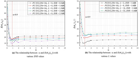
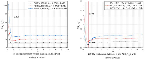
Figure 4.
The relationship between and with various decoding conditions.
4.2. Simulation Results and Performance Analysis
4.2.1. Error Correction Performance Analysis
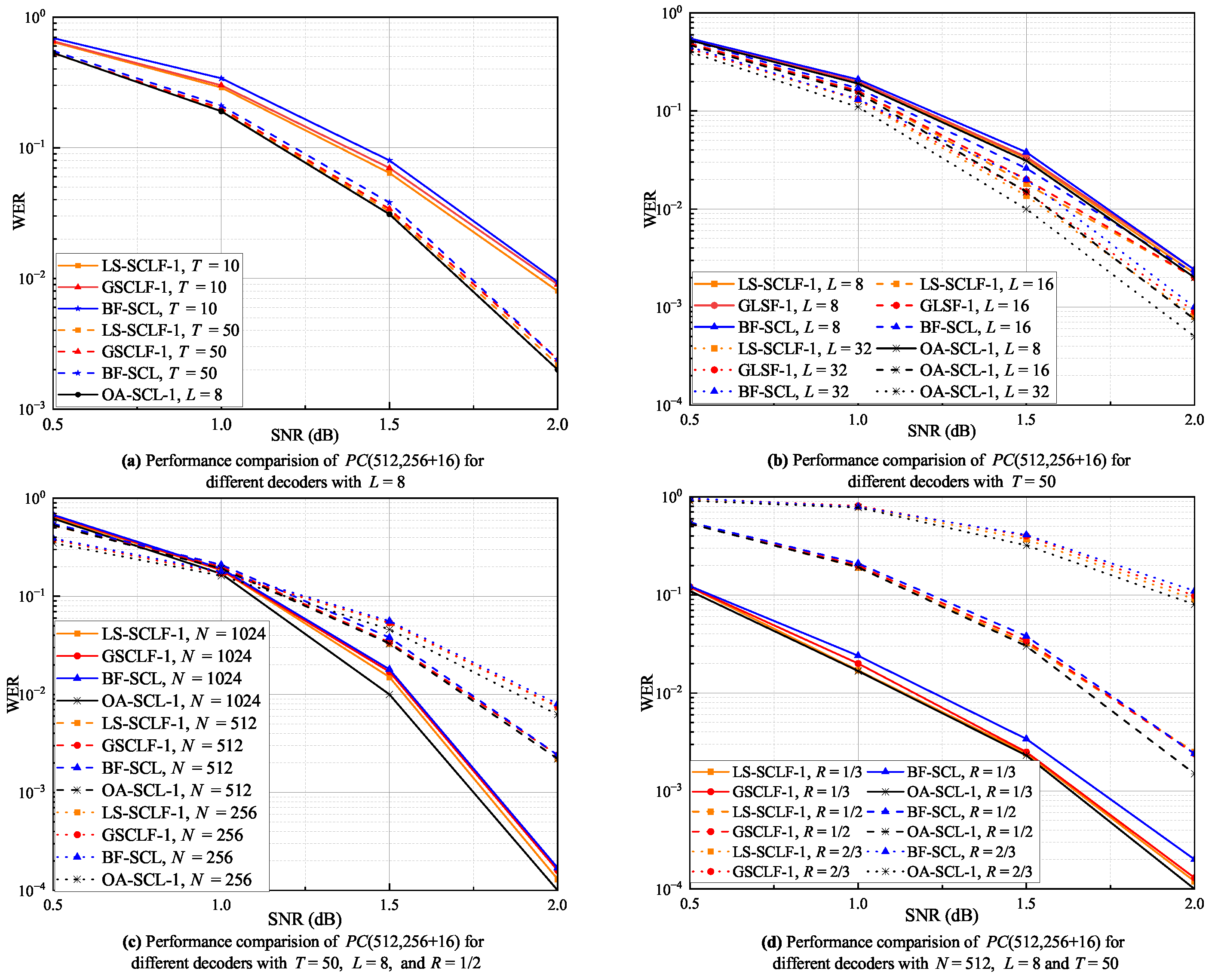
To verify the error correction performance of decoding, we simulate it for different conditions and compare it with BF-SCL decoding [30], GSCLF- decoding [31], and oracle-assisted SCL-() decoding, where the decoding corresponds to the genie-aided SCL decoding in [31]. In the paper, we choose to perform experiments on each of the above decoders. The WER curves for the decoding, decoding, and BF-SCL decoding under different T, L, N, and R conditions are shown in (a), (b), (c), and (d), respectively, in Figure 5. From Figure 5a, all the WER curves of the above decoders decrease as T increases, and the WER performance of the and decoders is better than that of the BF-SCL decoder. At , the WER values of the decoder are slightly lower than those of the decoder. At , the WER values of the both decoders are basically the same and very close to the WER values of the BF-SCL decoder. From Figure 5b, the WER curves of all the decoders decrease as the L increases, and the WER performance of the and decoders is better than that of the BF-SCL decoder. For , The WER curves of the and decoders are basically the same and very close to the WER curve of the OA-SCL-1 decoder. For and , the WER values of the decoder are slightly lower than those of the decoder, especially in the regions of 1.0 dB, where the difference between the two is more obvious. As can be seen in Figure 5c, almost all the WER curves for these decoders roughly intersect at dB. In the regions of dB, the WER values increase as the N increases and vice versa in the dB regions. In addition, at and , the WER curves of the and decoders are basically the same and slightly higher than that of the OA-SCL-1 decoder, while at , the WER curve of the decoder is slightly lower than that of the decoder in the regions of 1.0 dB. As illustrated in Figure 5d, when , the WER values of the decoder are slightly lower than those of the decoder, especially in the regions of 1.0 dB, and the difference between the two is more obvious. When and , the WER values of the decoder are approximately the same as those of the decoder, but in the regions around dB, the WER values of the decoder are lower than those of the decoder. In summary, Figure 5 shows that the LS-SCLF-1 decoder can correct more decoding caused by a single erroneous bit with the same number of extra decoding than the decoder, further proving the effectiveness of the bit-flipping metric and perturbation parameter optimization proposed in this paper. This also implies that the LS-SCLF decoder will also perform better for correcting higher-order erroneous bits.
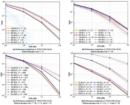
Figure 5.
WER curves for different decoders under various decoding conditions with .
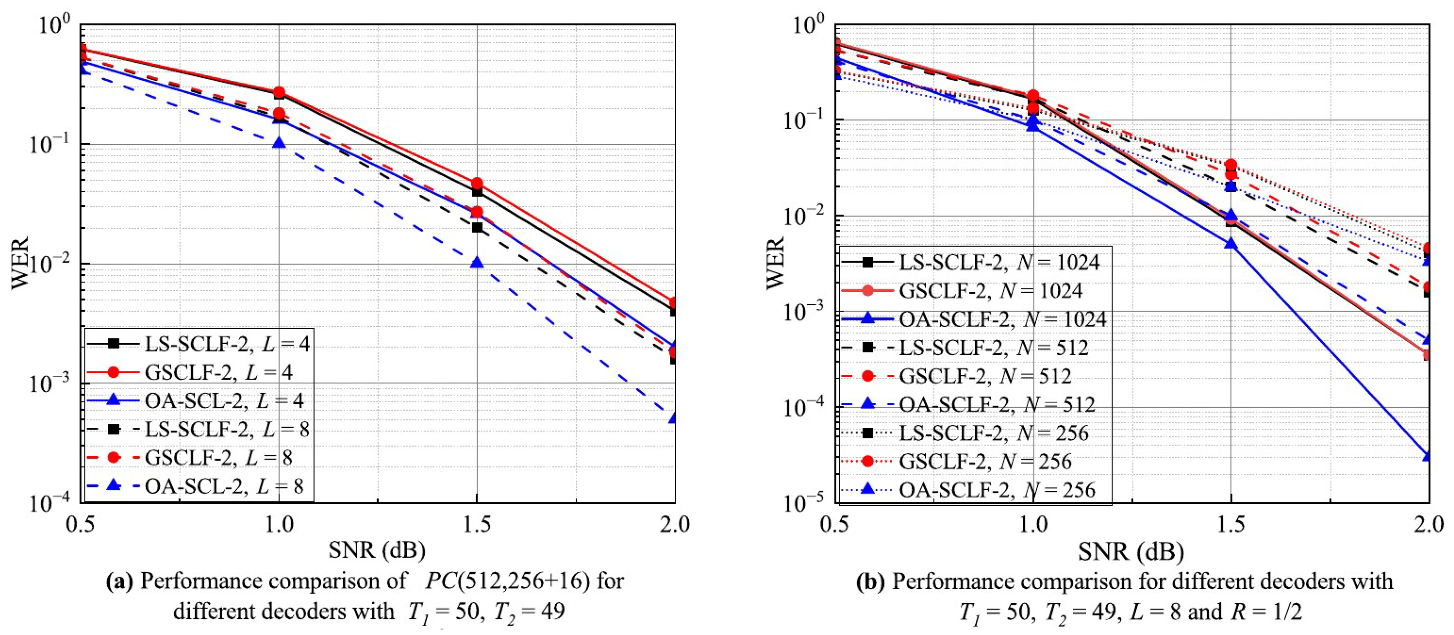
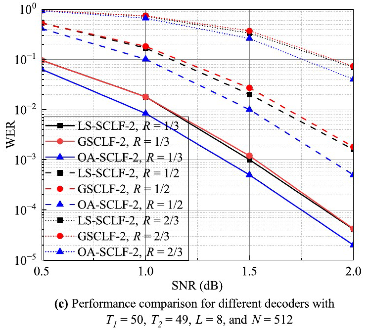
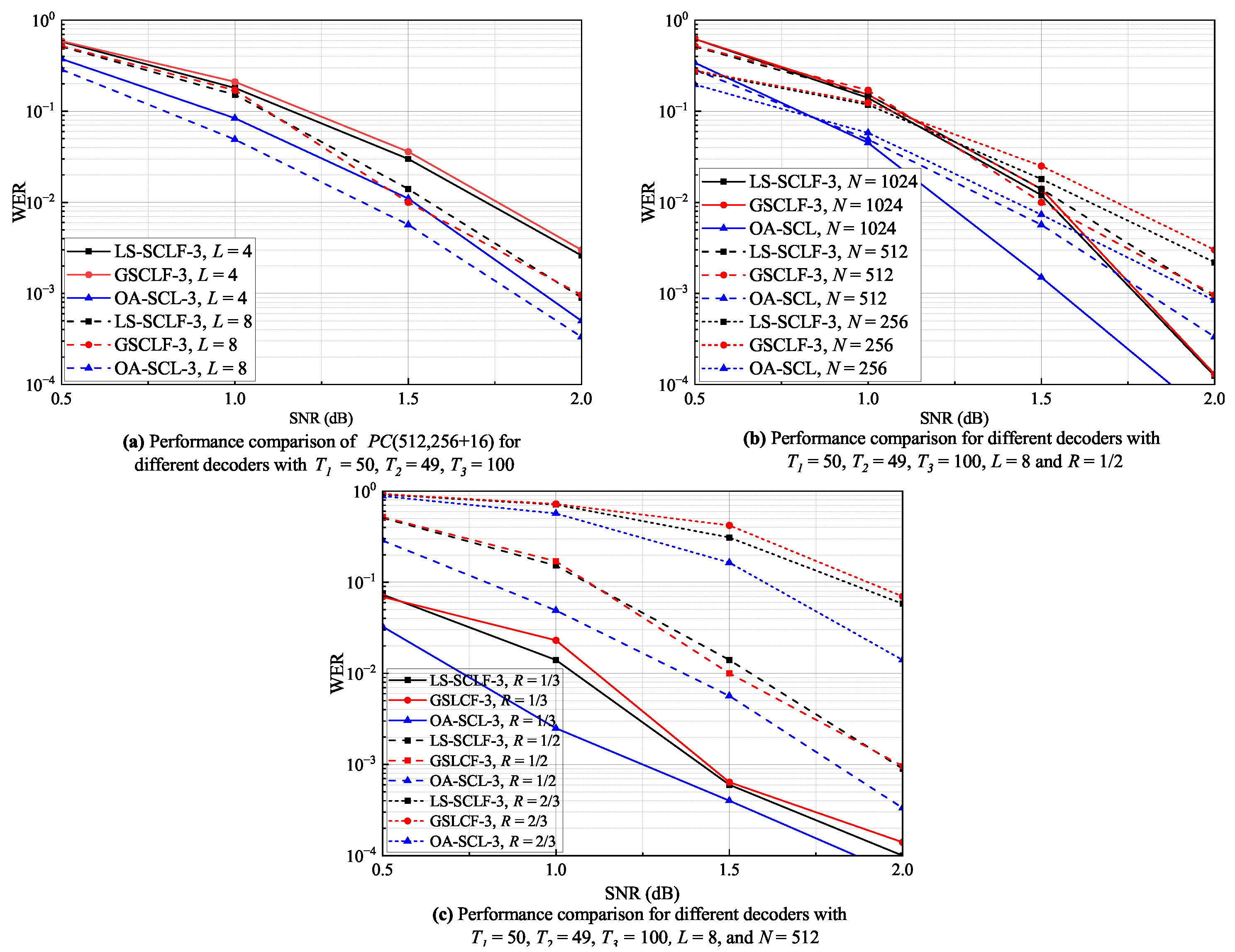
Figure 6a–c show the WER performance of LS-SCLF-2 decoding and decoding for various L, N, and R values. From Figure 6a, it can be seen that the WER values of the decoder are lower than those of the decoder in the 1.0 dB regions for both and . From Figure 6b, it can be seen that the WER curves of the decoder and the decoder are basically the same at and , while the WER values of the decoder are slightly lower than those of the decoder at . As can be seen in Figure 6c, the WER curves of the decoder are lower than those of the decoder under different R values, and the difference between them gradually increases with increasing . In summary, the overall error correction performance of the decoder is higher than that of the decoder, and the advantage of the decoder is more obvious in the region of 1.0 dB. Figure 7 shows the comparison of the error correction performance of different decoders at , where , , . Analyzing Figure 7, we can come to a similar conclusion as in Figure 5 and Figure 6; i.e., the error correction performance of the LS-SCLF-3 decoder is slightly better than that of the decoder under different decoding conditions.
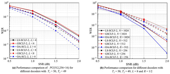
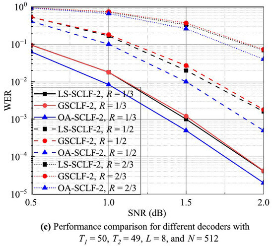
Figure 6.
WER curves for different decoders under various decoding conditions with .
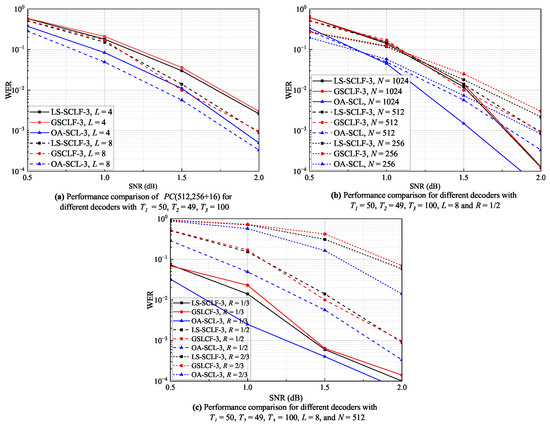
Figure 7.
WER curves for different decoders under various decoding conditions with .
4.2.2. Decoding Complexity Analysis
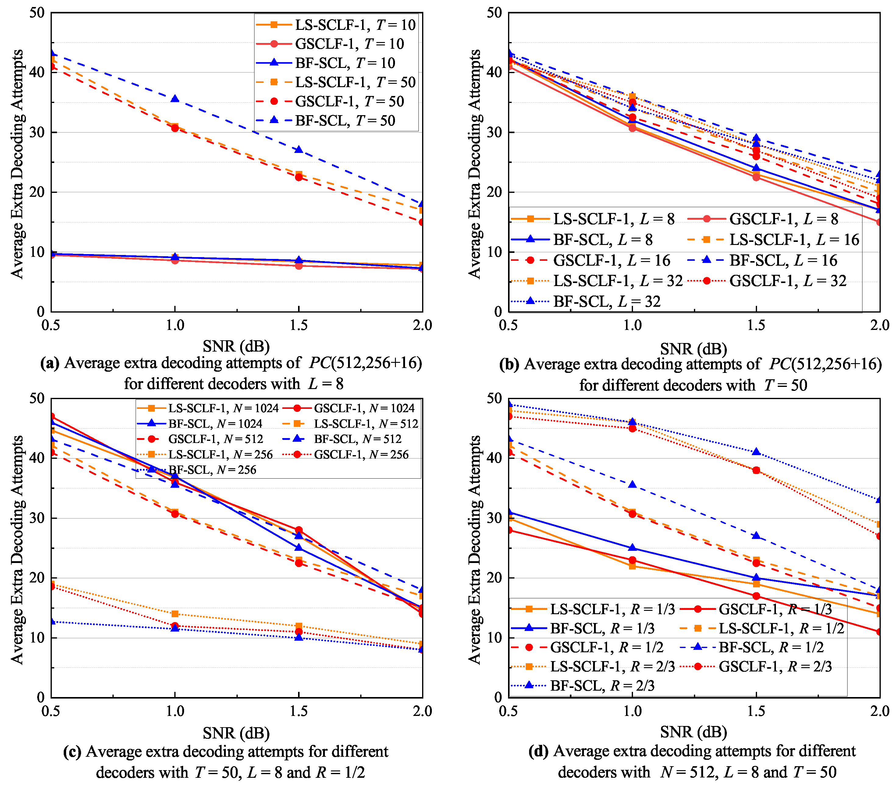
The complexity of bit-flipping-based SCL decoding is mainly composed of two parts: the flipping priority determination complexity and the extra decoding complexity, where the former is much smaller than the latter, especially with a large list size. Therefore, this paper mainly considers the extra decoding complexity, which can be expressed as , where is denoted as the average number of extra decoding attempts. It is clear that the average number of extra decoding attempts determines the complexity of the decoding, and this subsection focuses on the average number of extra decoding attempts. Figure 8, Figure 9 and Figure 10 show the corresponding average extra decoding attempts for Figure 5, Figure 6, and Figure 7, respectively.
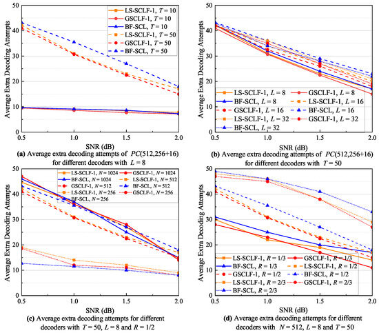
Figure 8.
Average extra decoding attempts of decoders under various decoding conditions with .
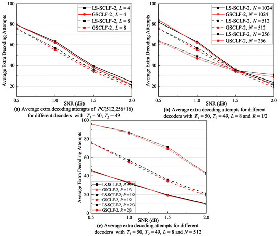
Figure 9.
Average extra decoding attempts of decoders under various decoding conditions with .
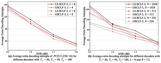
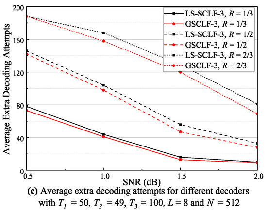
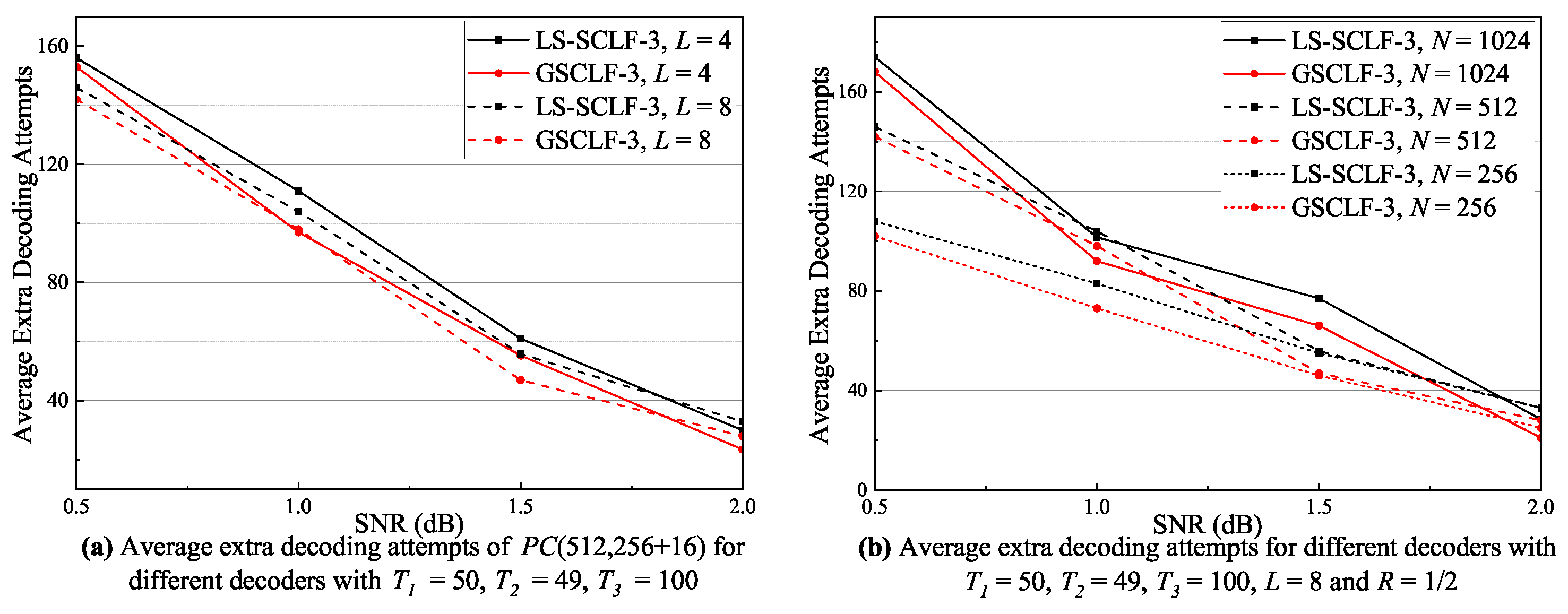
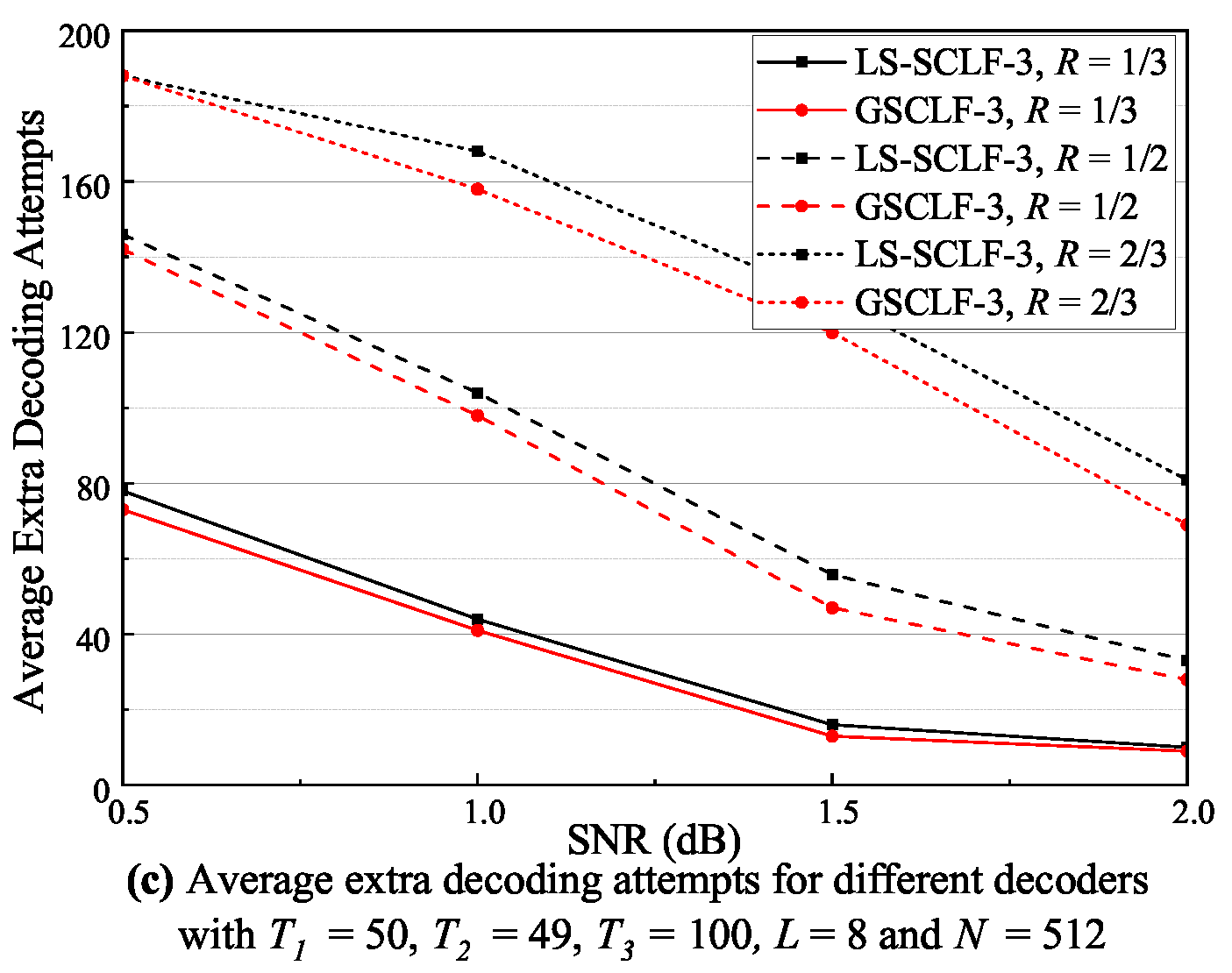
Figure 10.
Average extra decoding attempts of decoders under various decoding conditions with .
From Figure 8a, at , the decoders BF-SCL, , and exhibit an equivalent average number of extra decoding attempts. At , the BF-SCL decoder shows the largest number of extra decoding attempts, whereas the and decoders have similar average extra decoding attempts. As can be seen from Figure 8b, under different L conditions, the average extra decoding attempt curves of the decoder are all between those of the BF-SCL and decoders, indicating that the extra decoding complexity of decoder is smaller than that of the decoder and larger than that of the BF-SCL decoder. In the regions of 1.5 dB, the difference between the and decoders gradually increases, but with , for example, the difference between them is no more than 3. From Figure 8c, when and , the average extra decoding attempts of the and decoders are approximately the same, and both of them are smaller than those of the BF-SCL decoder. When , the average extra decoding attempts of decoder are slightly larger than those of the decoder, but both of them are higher than the average extra decoding attempts of the BF-SCL decoder. As can be seen from Figure 8d, the average extra decoding attempts of the BF-SCL decoder are higher than those of the other two decoders under different R conditions. The decoder also needs more extra decoding attempts than the decoder, and in the regions of 1.5 dB, the difference between them slightly increases, but it does not exceed 4. Based on the analysis of Figure 8, it can be concluded that overall, the BF-SCL decoder has the highest extra decoding complexity, while the decoder has slightly higher extra decoding complexity than the decoder.
As shown in Figure 9a, the average extra decoding attempts for the LS-SCLF-2 decoder are marginally greater than for the decoder at varying L conditions. The discrepancy between the two is more noticeable at , but it does not exceed 2 at the most. As shown in Figure 9b, the average extra decoding attempts of the LS-SCLF-2 decoder and the decoder are nearly equal under varying N conditions, and the six curves converge around dB. However, the difference between the average extra decoding attempts of the two decoder marginally rises in the 1.5 dB regions in comparison with other regions. From Figure 9c, we can see that the extra decoding attempts of both decoders rises considerably as R increases. For R values of one-third, the average extra decoding attempts for the LS-SCLF-2 decoder and the decoder are almost identical, but for values greater than one-half, the average extra decoding attempts of the LS-SCLF-2 decoder are marginally larger than those of the decoder. The analysis in Figure 9 demonstrates that the decoding complexity of the LS-SCLF-2 decoder is slightly greater than that of the decoder. In Figure 10, we can also observe a similar phenomenon as in Figure 9; i.e., when , the average number of extra decoding attempts of the LS-SCLF decoder is higher than those of the GSCLF decoding under different conditions, indicating that the LS-SCLF decoder has a higher average extra decoding complexity compared to the GSCLF decoder. However, the difference is that the gap between the average extra decoding attempts of the two decoders is much larger with ; e.g., in Figure 10b, when , the gap between them can reach more than 10 in the regions of 1.0 dB.
5. Conclusions
In this paper, we propose decoding. which can simultaneously correct erroneous decoded bits. Firstly, a new flip-bit metric is proposed. The metric takes into account the sequential nature of SCL decoding, i.e., the effect of the previous decoded bits on the bits to be decoded is introduced into the calculation of the metric. Then, a perturbation parameter is also introduced to make the metric as close as possible to the error probability of the flip-bit. Finally, a bit-flipping strategy is proposed, which searches and locates the erroneous decoded bits sequentially from lower to higher orders. Simulation results show that the LS-SCLF-1 decoder has better performance than the BF-SCL decoder in both error correction and decoding complexity. The decoder has better error correction performance than the decoder, especially at the medium to high regions, but its decoding complexity is slightly higher. In a word, the proposed decoder can achieve a good balance between the error correction performance and decoding complexity.
However, the perturbation parameter involved in this paper needs to be optimized through a large number of simulations. Meanwhile, the optimized parameter is not the optimal value under all conditions; for example, in Figure 4d, for , is its optimal parameter value, while is only a sub-optimal value under all conditions considered in a comprehensive way, which is the reason why the complexity of the proposed decoding algorithm is higher than that of the GSCLF decoder. To solve this problem, we hope to improve the decoding algorithm in the following ways in future work. (1) To reduce the excessive occupation of computing resources, the optimized parameter can be stored in the system in advance. (2) The parameter optimization problem can be solved from a theoretical point of view. The functional relationship between different decoding conditions and the corresponding optimal parameter values is summarized so as to avoid the instability caused by experimental statistics.
Author Contributions
Conceptualization, D.W., J.Y., Y.X. and G.H.; methodology, D.W., J.Y. and Y.X.; software, D.W., Q.X. and X.Y.; validation, Q.X. and X.Y.; supervision, J.Y., Y.X. and G.H.; funding acquisition, J.Y., Y.X. and G.H. All authors have read and agreed to the published version of the manuscript.
Funding
National Natural Science Foundation of China: 62271446, 51574232;
Xinjiang Key Research and Development Special Task: 2022B03003-3.
Data Availability Statement
Not applicable.
Conflicts of Interest
The authors declare no conflict of interest.
References
- Erdal, A. Channel Polarization: A Method for Constructing Capacity-Achieving Codes for Symmetric Binary-Input. IEEE Trans. Inf. Theory 2009, 55, 3051–3073. [Google Scholar]
- Lidström, V. Low-density parity-check codes. IEEE Trans. Inf. Theory. 1962, 12, 21–28. [Google Scholar]
- Berrou, C.; Glavieux, A. Near Shannon limit error-correcting coding and decoding: Turbo-codes. In Proceedings of the ICC 93-IEEE International Conference on Communications, Geneva, Switzerland, 23–26 May 1993. [Google Scholar]
- Liang, H.; Liu, A.; Tong, X.; Gong, C. Raptor-like Rateless Spinal Codes using Outer Systematic Polar Codes for Reliable Deep Space Communications. In Proceedings of the IEEE INFOCOM 2020—IEEE Conference on Computer Communications Workshops (INFOCOM WKSHPS), Toronto, ON, Canada, 6–9 July 2020; pp. 1045–1050. [Google Scholar]
- Feng, B.; Jiao, J.; Wu, S.; Zhang, Q. How to apply polar codes in high throughput space communications. Sci. China Tech. Sci. 2020, 63, 1371–1382. [Google Scholar] [CrossRef]
- Zhai, Y.; Li, J.; Feng, H.; Hong, F. Application research of polar coded OFDM underwater acoustic communications. J. Wireless. Com. Netw. 2020, 63, 1371–1382. [Google Scholar] [CrossRef]
- Liu, F.; Wu, Q.; Li, C.; Chen, F.; Xu, Y. Polar Coding Aided by Adaptive Channel Equalization for Underwater Acoustic Communication. IEICE Tech. Fund. Electr. 2023, E106.A, 83–87. [Google Scholar] [CrossRef]
- Lidstrom, V. Evaluation of Polar-Coded Noncoherent Acoustic Underwater Communication. IEEE J. Ocean. Eng. 2023, 2023, 1–14. [Google Scholar] [CrossRef]
- Wang, H.; Kim, S. Dimming Control Systems with Polar Codes in Visible Light Communication. IEEE Photonics Technol. Lett. 2017, 29, 1651–1654. [Google Scholar] [CrossRef]
- Wang, H.; Kim, S. Design of Polar Codes for Run-Length Limited Codes in Visible Light Communications. IEEE Photonics Technol. Lett. 2019, 31, 27–30. [Google Scholar] [CrossRef]
- Wang, H.; Kim, S. Adaptive Puncturing Method for Dimming in Visible Light Communication with Polar Codes. IEEE Photonics Technol. Lett. 2018, 30, 1780–1783. [Google Scholar] [CrossRef]
- Zheng, H.; Wu, K.; Chen, B. Experimental Demonstration of 9.6 Gbit/s Polar Coded Infrared Light Communication System. IEEE Photonics Technol. Lett. 2020, 32, 1539–1542. [Google Scholar] [CrossRef]
- Tal, I.; Vardy, A. List Decoding of Polar Codes. IEEE Trans. Inf. Theory 2015, 61, 2213–2226. [Google Scholar] [CrossRef]
- Niu, K.; Chen, K. CRC-Aided Decoding of Polar Codes. IEEE Commun. Lett. 2012, 16, 1668–1671. [Google Scholar] [CrossRef]
- Li, B.; Shen, H.; Tse, D. An Adaptive Successive Cancellation List Decoder for Polar Codes with Cyclic Redundancy Check. IEEE Commun. Lett. 2012, 16, 2044–2047. [Google Scholar] [CrossRef]
- Gao, C.; Liu, R.; Dai, B.; Han, X. Path Splitting Selecting Strategy-Aided Successive Cancellation List Algorithm for Polar Codes. IEEE Commun. Lett. 2019, 23, 422–425. [Google Scholar] [CrossRef]
- Wang, X.; Zhang, H.; Li, J.; Bao, X.; Xie, K. An Improved Path Splitting Decision-Aided SCL Decoding Algorithm for Polar Codes. IEEE Commun. Lett. 2021, 25, 3463–3467. [Google Scholar] [CrossRef]
- Zhang, Z.; Zhang, L.; Wang, X.; Zhong, C.; Poor, H.V. A Split-Reduced Successive Cancellation List Decoder for Polar Codes. IEEE J. Sel. Areas Commun. 2016, 34, 292–302. [Google Scholar] [CrossRef]
- Doan, N.; Hashemi, S.A.; Gross, W.J. Fast Successive-Cancellation List Flip Decoding of Polar Codes. IEEE Access 2022, 10, 5568–5584. [Google Scholar] [CrossRef]
- Ardakani, M.H.; Hanif, M.; Ardakani, M.; Tellambura, C. Fast Successive-Cancellation-Based Decoders of Polar Codes. IEEE Trans. Commun. 2019, 67, 4562–4574. [Google Scholar] [CrossRef]
- Sarkis, G.; Giard, P.; Vardy, A.; Thibeault, C.; Gross, W.J. Fast List Decoders for Polar Codes. IEEE J. Sel. Areas Commun. 2016, 34, 318–328. [Google Scholar] [CrossRef]
- Afisiadis, O. A low-complexity improved successive cancellation decoder for polar codes. In Proceedings of the 2014 48th Asilomar Conference on Signals, Systems and Computers, Pacific Grove, CA, USA, 2–5 November 2014; pp. 2116–2120. [Google Scholar]
- Ercan, F.; Condo, C.; Gross, W.J. Improved Bit-Flipping Algorithm for Successive Cancellation Decoding of Polar Codes. IEEE Trans. Commun. 2019, 67, 61–72. [Google Scholar] [CrossRef]
- Condo, C.; Ercan, F.; Gross, W.J. Improved Successive Cancellation Flip Decoding of Polar Codes Based on Error Distribution. In Proceedings of the 2018 IEEE Wireless Communications and Networking Conference Workshops (WCNCW), Barcelona, Spain, 15–18 April 2018; pp. 19–24. [Google Scholar]
- Zhang, Z.; Qin, K.; Zhang, L.; Chen, G.T. Progressive Bit-Flipping Decoding of Polar Codes: A Critical-Set Based Tree Search Approach. IEEE Access 2018, 6, 57738–57750. [Google Scholar] [CrossRef]
- Wang, D.; Yin, J.; Xu, Y.; Yang, X.; Hua, G. Threshold Based D-SCFlip Decoding of Polar Codes. IEICE Trans. Commun. 2023, E106.B, 635–644. [Google Scholar] [CrossRef]
- Chandesris, L.; Savin, V.; Declercq, D. Dynamic-SCFlip Decoding of Polar Codes. IEEE Trans. Commun. 2018, 66, 2333–2345. [Google Scholar] [CrossRef]
- Yu, Y.Y.; Pan, Z.W.; Liu, N.; You, X.H. Successive Cancellation List Bit-flip Decoder for Polar Codes. In Proceedings of the 2018 10th International Conference on Wireless Communications and Signal Processing (WCSP), Hangzhou, China, 18–20 October 2018; pp. 1–6.
- Rowshan, M.; Viterbo, E. Shifted Pruning for Path Recovery in List Decoding of Polar Codes. In Proceedings of the 2021 IEEE 11th Annual Computing and Communication Workshop and Conference (CCWC), Las Vegas, NV, USA, 27–30 January 2021; pp. 1179–1184. [Google Scholar]
- Cheng, F.; Liu, A.; Ren, J.D. Bit-Flip Algorithm for Successive Cancellation List Decoder of Polar Codes. IEEE Access 2019, 7, 58346–58352. [Google Scholar] [CrossRef]
- Pan, Y.H.; Wang, C.H.; Ueng, Y.L. Generalized SCL-Flip Decoding of Polar Codes. In Proceedings of the GLOBECOM 2020—2020 IEEE Global Communications Conference, Taipei, Taiwan, 7–11 December 2020; pp. 1–6. [Google Scholar]
- Balatsoukas-Stimming, A.; Parizi, M.B.; Burg, A. LLR-Based Successive Cancellation List Decoding of Polar Codes. IEEE Trans. Signal. Process. 2015, 63, 5165–5179. [Google Scholar] [CrossRef]


Disclaimer/Publisher’s Note: The statements, opinions and data contained in all publications are solely those of the individual author(s) and contributor(s) and not of MDPI and/or the editor(s). MDPI and/or the editor(s) disclaim responsibility for any injury to people or property resulting from any ideas, methods, instructions or products referred to in the content. |
© 2023 by the authors. Licensee MDPI, Basel, Switzerland. This article is an open access article distributed under the terms and conditions of the Creative Commons Attribution (CC BY) license (https://creativecommons.org/licenses/by/4.0/).