Analysis of Decision-Making in a Green Supply Chain under Different Carbon Tax Policies

Abstract

With the growing severity of global environmental issues, the international community has reached a consensus on the importance of reducing and controlling carbon emissions. As a result, an increasing number of consumers are opting to purchase green products in order to reduce the emission of greenhouse gases. This trend has prompted supply-chain enterprises to invest in green innovation. Simultaneously, carbon tax policies have gained significant attention from governments worldwide due to their dual role as environmental laws and fiscal-policy tools. Considering consumers’ preference for green products and the risk of R&D failure associated with them, this study focuses on the effects on emissions reductions and profits associated with different carbon tax policies for a green supply chain consisting of a manufacturer and a retailer. The results reveal that (1) increases in the carbon tax per unit of product motivate the manufacturer to increase R&D efforts; (2) wholesale and retail prices follow a pattern of initial increase and subsequent decrease as the carbon tax per unit of product rises; (3) higher carbon taxes per unit of product generally lead to lower manufacturer profits, while both carbon emissions and retailer profits can increase with a per-unit carbon tax under certain circumstances; and (4) the increase in the proportion of the population with green preferences can yield long-term benefits for both the retailer and the manufacturer, yielding an inverted U-shaped relationship with carbon emissions.

1. Introduction

With rapid economic development, increasing resource scarcity, and worsening environmental pollution, there is a growing consensus among countries regarding the need to prioritize green development [1]. In this context, consumer preferences are shifting toward green products and the perception of products as green has a significant influence on purchasing decisions [2]. Compared to conventional products, green products require more investment in green innovation, and their degree of environmental friendliness affects both product price and demand [3]. Fussler and James [4] first formally proposed the concept of green innovation to refer to the research, design, and production of environmentally friendly products. There is also a risk of R&D failure for green products that can be attributed to the substantial investments required for green innovation, extended payback periods, and comparatively higher prices of green products [5]. However, as consumer preference for green products continues to grow, it serves to stimulate consumer demand for such offerings and foster consumer acceptance of the price premiums. Consequently, this surge in demand not only increases manufacturers’ profits, but also prompts them to intensify investments in green innovation. On the one hand, the growth of investment facilitates the advancement of green innovation technologies, resulting in shorter payback periods. On the other hand, as production scales up in response to increased investment, economies of scale come into play, reducing production costs and subsequently lowering the prices of green products. Accordingly, the risk of R&D failure diminishes as consumer preferences for green products rise. Therefore, this paper aims to explore the optimal balance between minimizing green innovation investment and maximizing benefits for the members of the green supply chain under expanding consumer demand.

In light of the increasingly severe issue of global warming, reducing carbon emissions has been recognized as an effective approach to addressing climate change. Governments worldwide have introduced corresponding policies to effectively control carbon emissions. China, for instance, has made international commitments to achieve its carbon peak by 2030 and carbon neutrality by 2060. Similarly, countries like the UK, France, and Canada have implemented various policies and regulations to reduce carbon emissions. Among these policies, the carbon tax been widely adopted by governments due to its effectiveness and ease of implementation [6]. Moreover, implementing differentiated carbon regulations based on different levels of carbon emissions has shown significant emission-reduction effects in practice [7,8]. The consumer preference for green products, along with the manufacturer’s investments in green innovation, act as internal drivers reducing carbon emissions. Simultaneously, the government’s implementation of a carbon tax policy serves as an external constraint in the context of carbon-emission reduction. Therefore, studying the decision-making processes within green supply chains that encompass both internal and external considerations assumes great significance and relevance.

In recent years, scholars have conducted extensive, in-depth research on green supply-chain issues, considering the impact of consumers’ behavior related to green preferences and carbon tax policies. Regarding the greenness of products in the context of green supply chains, various studies have examined the coordination mechanisms. Ghosh and Shah [9] explore the impact of cost-sharing contracts within a single-channel structure on the greenness of products, pricing, and profitability for participants in the supply chain. Li et al. [10] analyze the dual-channel structure in a green supply chain and investigate firms’ pricing strategies. Gao et al. [11] develop a game model for a two-tiered green supply chain under different rights structures and investigate the changes in the equilibrium solution to the game using the revenue-sharing mechanism. Zhang and Liu [12] extend these studies to a three-level green supply-chain model. Behavioral factors such as fairness preference and risk aversion have also been incorporated into green supply-chain research. Zhou et al. [13] and Jiang et al. [14] introduce these factors to study their impact on green supply chains. Furthermore, Liu and Yi [15] and Liu et al. [16] examine pricing strategies in green supply chains in the context of big data and blockchain environments, respectively. Yang and Xiao [17] analyze the issue of low-carbon supply-chain channel selection. Some scholars have studied the supply chain from the perspective of collaborative R&D. Zhou et al. (2020) [18] discuss supply-chain equilibrium strategies under different R&D models, considering whether green supply-chain members collaborate on R&D. Lin [19] investigates the impact of investment sharing and innovation-sharing cooperative behaviors among competitors on the price of green products, environmental quality, and firm-level business decisions. Additionally, Zhu and He [20] examine how the structure of the supply chain affects R&D decisions related to green products.

In the field of carbon tax-policy research, scholars have examined the impact of such policies on supply-chain carbon emission-reduction strategies [21,22] and production decision-making [23] under a single channel. With the successful implementation of dual-channel supply chains, researchers have started to integrate the carbon-tax mechanism into dual-channel supply chain research. Scholars have extensively explored issues such as dual-channel selection, emission-reduction decisions, pricing decisions, and coordination in dual-channel supply chains [18,24,25,26,27,28]. Furthermore, Jaber et al. [29] suggest that a hybrid carbon policy combining a carbon tax and carbon penalties may be the most effective emission-reduction strategy. Several scholars have examined the operational mechanisms and emission-reduction strategies of supply chains under hybrid carbon policies [30,31,32,33,34]. Undoubtedly, the implementation of a carbon tax policy plays a crucial role in facilitating structural transformation in industries, but its effects on economic growth can be somewhat negative. However, research conducted by Li and Han [35] suggests that the negative impact of the carbon tax policy can be effectively mitigated through carbon tax subsidies. Chen and Hu [36] and Guo and Huang [37] discover that under certain conditions, carbon taxes are more effective than carbon tax subsidies in promoting low-carbon manufacturing and enhancing social welfare. Meng [38] demonstrates that social welfare is higher when R&D subsidies are adopted under very low or very high carbon tax rates. Vaughan et al. [39] and Qiu et al. [40] investigate the specific impacts of carbon tax incentives in the fisheries sector and the passenger air-transport industry, respectively. These findings highlight the potential of incentives to stimulate economic growth while reducing carbon emissions. These studies contribute to our understanding of how carbon-tax policies can impact supply chains and provide insights into decision-making and emission-reduction strategies in the context of both single-channel and dual-channel supply chains.

A review of the literature has revealed substantial research on carbon tax policies and consumer green preferences in supply chains. Nevertheless, there is no existing literature that simultaneously integrates the risk of R&D failure in green innovation and that a carbon tax policy that restricts carbon emissions within green supply chains. Based on the existing literature, this paper incorporates the risk of R&D failure into the framework of carbon tax policy and considers the optimal decision-making processes in green supply chains. Moreover, we evaluate the impacts of different carbon tax policies and the degree of green preference on the profitability and carbon emissions of green supply chains.

This paper contributes to the following aspects: (1) To the best of our knowledge, we consider for the first time the distribution of consumers’ green preferences with a specific focus on its effect on price sensitivity. (2) Within the context of green development, this research analyzes the influence of different carbon tax policies on profits and carbon emissions among supply chain firms. The findings of this study can offer a scientific basis and theoretical guidance for the formulation of carbon tax policies and the selection of enterprises’ production decisions. (3) This paper investigates the optimal strategy for green supply chains while accounting for the risk of R&D failure, thus ensuring the model’s alignment with real-world scenarios. (4) We derive some counterintuitive and interesting results, such as the finding that the implementation of a carbon tax policy and an increased presence of green-preferring consumers do not necessarily lead to a reduction in carbon emissions. Additionally, we extensively explore the conditions under which carbon tax policies can increase supply-chain profits.

The remainder of the paper is organized as follows. Section 2 presents the formulation of the problem and provides a comprehensive discussion of the underlying model. In Section 3, we delve into the distinction between a uniform carbon tax policy and a non-uniform carbon tax policy. Section 4 comprises the sensitivity analysis. Section 5 provides a real-life study case on Denmark. Finally, the conclusions are presented in Section 6.

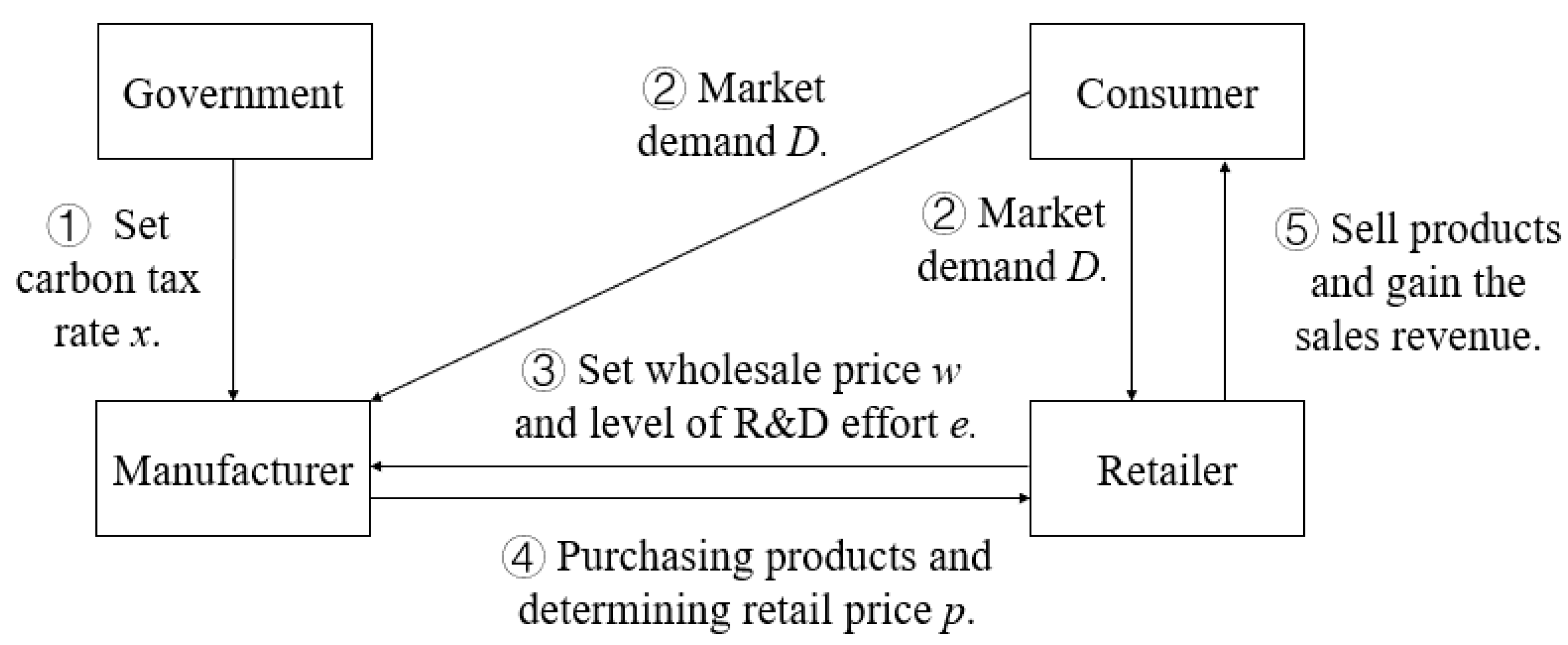
2. Problem Description and Assumptions

Consider a green supply chain consisting of a manufacturer, denoted as M, and a retailer, denoted as R. The manufacturer is responsible for producing the green product, and the retailer is responsible for selling it to the final consumer ailer. In the production process, the government imposes a carbon tax on the carbon emissions generated by the manufacturer. On one hand, consumers are willing to pay higher prices for products with lower carbon emissions due to their green preference [9]. On the other hand, the manufacturer aims to develop low-carbon products through green-innovation R&D to reduce carbon tax expenses and production costs. However, there is an uncertainty associated with the R&D of low-carbon-emission products, with a probability of success, $e(0\le e\le 1)$, and a probability of failure, $1-e$ [5,41]. The costs of R&D are directly linked to the level of R&D effort (probability of success), assumed to be $s{e}_1{}^2/2$. If the R&D is successful, the manufacturer can reduce the initial carbon emissions from $tD$ to $(1-b)tD$. The demand for green products in the market is influenced by both the price and the carbon emissions [2,42]. We assume that the market demand function for green products is represented by the formula

$$D=a-dp+\lambda e,$$

(1)

where $a-dp>0$.

We assume that only a proportion $\theta (\theta \in [0,1])$ of consumers have a preference for green products and that among those consumers, the degree of green preference may vary. Consumers with higher levels of green preference exhibit lower sensitivity to the price of green products. To quantify the degree of preference for green products among consumers, we introduce the parameter $\tau$, which is uniformly distributed on $[1-\theta ,1]$ [43]. Assuming that $d=u\tau$, we can obtain the formula

$$E(d)=u\frac{2-\theta }{2}.$$

(2)

Therefore, the expected demand function is

$$E(D)=a-E(d)p+\lambda e.$$

(3)

To simplify the analysis, we introduce the following additional assumptions. (1) In the supply chain, the manufacturer assumes the role of the leader, while the retailer acts as the follower. (2) The manufacturer’s per-unit manufacturing costs remain constant throughout the analysis. Additionally, the investment in emission-reduction R&D is a one-time event that occurs at the beginning of the period. If the R&D is successful, the carbon emissions can be reduced to the expected value. (3) The market supply is equal to the market demand, implying that there are no inventory levels or stock-outs. (4) Information within the supply chain is symmetric, meaning that both the manufacturer and the retailer have access to the same information. (5) We assume there is no salvage value at the end of the selling period and that only one order can be placed.

The primary aim of this paper is to examine and answer three key questions. Firstly, how does the implementation of carbon tax policies affect the level of R&D efforts and market prices? Secondly, in the context of green development, can increasing the proportion of consumers with green preferences result in a win-win situation for supply-chain firms in terms of economic profit and emission reduction? Lastly, does the change in carbon tax policy encourage supply chains to implement energy saving and emission reduction, while promoting profit growth?

Table 1. List of notations.

Symbol	Definition
Parameters
c	Unit production cost
D	Total market demand
a	Potential market demand
d	Influence of sales price on demand
λ	Influence of R&D effort on demand
s	Cost parameter for R&D effort
x	Carbon tax rates
t	Carbon emissions per unit of product
b	Carbon-emission reduction rate
θ	Proportion of population with a green preference for consumers
τ	Level of preference of green-preference consumers
u	Influence of green-preference level on price sensitivity
m	Proportion of fossil energy with high carbon content
n	Proportion of carbon emissions from production
z	Carbon tax on carbon emissions from production
${\pi }_j$	Profit of firms (j = M, R)
Decision variables
w	The product’s wholesale price
e	Level of R&D effort
p	The product’s sales price

provides a detailed description of the parameters used in this study.

3. Model

3.1. The Model with a Uniform Carbon Tax

Figure 1 illustrates the sequential progression of events. Within the framework of the Stackelberg game, both the manufacturer and the retailer strive to maximize their profits. As the dominant player in this game, the manufacturer takes charge of making decisions in the first stage. The manufacturer determines the wholesale price ($w$) and the level of R&D effort ($e$). Following the manufacturer’s decision, the retailer observes these choices and subsequently determines the optimal retail price ($p$) in order to maximize their profit.

Under a uniform carbon tax policy, the manufacturer’s expected profit $E({\pi }_M)$ and the retailer’s expected profit $E({\pi }_R)$ are as follows:

$$E({\pi }_M)=(w-c)E(D)-\frac{1}{2}s{(e)}^2-(1-be)xtE(D),$$

(4)

$$E({\pi }_R)=(p-w)E(D).$$

(5)

Proposition 1.

The expected profits of the manufacturer and the retailer are concave functions of the decision variables. There are optimal values for both when $s>s_1=\frac{{(2\lambda +ubxt(2-\theta ))}^2}{8u(2-\theta )}$.

The first-order partial derivative of the retail price in the Equation (5) is

$$\frac{\partial {\pi }_R^{}}{\partial p}=a-u(2-\theta )p+\lambda e+\frac{u(2-\theta )}{2}w.$$

(6)

From $\frac{{\partial }^2{\pi }_R^{}}{{\partial }^{2}p}=-u(2-\theta )<0$, the retailer’s profit function is a concave function of $p$.

There exists an optimal value of $p$. Letting $\frac{\partial {\pi }_R^{}}{\partial p}=0$, we know that

$$p=\frac{2a+2\lambda e+u(2-\theta )w}{2u(2-\theta )}.$$

(7)

Combining Equations (4) and (7), we have the Hessian matrix of the manufacturer’s expected profit function for $e$ and $w$:

$$H=\left[\begin{array}{l}\frac{{\partial }^2{\pi }_M}{{\partial }^{2}e}\\ \frac{{\partial }^2{\pi }_M}{\partial w\partial e}\end{array}\right.\left.\begin{array}{l}\frac{{\partial }^2{\pi }_M}{\partial e\partial w}\\ \frac{{\partial }^2{\pi }_M}{{\partial }^{2}w}\end{array}\right]=\left[\begin{array}{l}-s+\lambda bxt\\ \frac{2\lambda -ubxt(2-\theta )}{4}\end{array}\right.\left.\begin{array}{l}\frac{2\lambda -ubxt(2-\theta )}{4}\\ -u\frac{2-\theta }{2}\end{array}\right].$$

The Hessian matrix is negative-semidefinite when $8su(2-\theta )-{(ubxt(2-\theta )+2\lambda )}^2>0$ and $-s+\lambda bxt<0$. Therefore, the manufacturer’s expected profit function is a joint concave function of $e$ and $w$ when $s>s_1=\frac{{(ubxt(2-\theta )+2\lambda )}^2}{8u(2-\theta )}$. At this point, there exist optimal solutions for $e$ and $w$.

Proposition 2.

The optimal solution for the decision variables is

$$e^{*}=\frac{(2a-u(2-\theta )(c+xt))(ubxt(2-\theta )+2\lambda )}{8us(2-\theta )-{(ubxt(2-\theta )+2\lambda )}^2},$$

(8)

$$w^{*}=\frac{4s(u(2-\theta )(c+xt)+2a)-2(ubxt(2-\theta )+2\lambda )(\lambda (c+xt)+abxt)}{8us(2-\theta )-{(ubxt(2-\theta )+2\lambda )}^2},$$

(9)

$$p^{*}=\frac{2s(u(2-\theta )(c+xt)+6a)-2(ubxt(2-\theta )+2\lambda )(\lambda (c+xt)+abxt)}{8us(2-\theta )-{(ubxt(2-\theta )+2\lambda )}^2}.$$

(10)

According to the inverse induction method, combining Equations (4) and (7), the first-order derivatives of $e$ and $w$ can be obtained as follows:

$$\frac{\partial {\pi }_M^{}}{\partial e}=\frac{1}{4}(2\lambda (w-c-xt)+bxt(2a-uw(2-\theta )))-(s-\lambda bxt)e,$$

(11)

$$\frac{\partial {\pi }_M^{}}{\partial w}=\frac{1}{4}(2a+2\lambda e+u(2-\theta )(c+xt(1-be)))-\frac{(2-\theta )}{2}w.$$

(12)

The optimal values of $e$ and $w$ can be obtained from $\frac{\partial {\pi }_M^{}}{\partial e}=0$ and $\frac{\partial {\pi }_M^{}}{\partial w}=0$, and the optimal value of $p$ can be obtained according to Equation (7), by substituting Equation (8) to Equation (10) into Equations (4) and (5), respectively.

$${\pi }_M^{*}=\frac{s{(2a-u(2-\theta )(c+xt))}^2}{16us(2-\theta )-2{(ubxt(2-\theta )+2\lambda )}^2},$$

(13)

$${\pi }_R^{*}=\frac{2u{s}^2(2-\theta ){(2a-u(2-\theta )(c+xt))}^2}{{(8us(2-\theta )-{(ubxt(2-\theta )+2\lambda )}^2)}^2}.$$

(14)

When $p^{*}$, $w^{*}$, ${\pi }_M^{*}$ and ${\pi }_R^{*}$ are all greater than 0 and $0<e^{*}\le 1$, the manufacturer and the retailer will produce and sell products. In order to fulfil the above conditions, we get $s\ge s_2=\frac{(2\lambda +ubxt(2-\theta ))(2a-u(2-\theta )(c+xt)+2\lambda +ubxt(2-\theta ))}{8u(2-\theta )}$ and $2a-u(2-\theta )(c+xt)>0$. Therefore, the subsequent analyses in this section will be conducted under the condition that $s\ge s_2$ because $s_2>s_1$. Otherwise, $e^{*}>1$ implies that the manufacturer must be successful in product innovation, which is inconsistent with the previous assumptions and with reality.

Corollary 1.

$\lambda \le ubxt(2-\theta )/2$.

Corollary 1 highlights that the manufacturer is incentivized to engage in green innovation when $\lambda \le ubxt(2-\theta )/2$ (see Appendix A for proof). In this scenario, the manufacturer’s profit after the innovation is implemented is guaranteed to be at least as high as the profit achieved without the innovation. If the expected profit after innovation were lower than the profit without innovation, the manufacturer would have no incentive to invest in measures to reduce carbon emissions.

Corollary 2.

(1) $\partial e^{*}/\partial s<0$, $\partial w^{*}/\partial s>0$, $\partial {\pi }_M^{*}/\partial s<0$, $\partial {\pi }_R^{*}/\partial s<0$.

(2) When $ubxt(2-\theta )/6<\lambda \le ubxt(2-\theta )/2$, $\partial p^{*}/\partial s<0$. When $\lambda \le ubxt(2-\theta )/6$, $\partial p^{*}/\partial s\ge 0$.

Corollary 2(1) demonstrates that as $s$ increases, the manufacturer’s optimal level of R&D effort decreases, whereas the optimal wholesale price moves in the opposite direction. This behavior can be attributed to the fact that the manufacturer’s investment in green innovation increases with $s$. Higher R&D costs decrease the incentive for green innovation, resulting in a reduction of the optimal level of R&D effort and an increase in the optimal wholesale price. Consequently, the optimal profit of the members of the supply chain decreases as s increases. In Corollary 2(2), it is shown that the optimal retail price decreases with $s$ when $\lambda$ is relatively high. We argue that a decrease in the level of R&D effort leads to a significant decline in consumer demand, prompting the retailer to lower prices in order to stimulate consumer interest and boost sales. Conversely, when $\lambda$ is small enough, the optimal retail price increases with $s$. At this time, we believe that a decrease in R&D effort will have a lesser negative impact on consumer demand. Facing increasing wholesale prices, the retailer will choose to raise retail prices in order to maintain profitability. Concrete proof can be seen in Appendix B.

Corollary 3.

(1) $\partial e^{*}/\partial \lambda >0$, $\partial {\pi }_M^{*}/\partial \lambda >0$, $\partial {\pi }_R^{*}/\partial \lambda >0$.

(2) When $\lambda (a-\frac{u(2-\theta )(c+xt)}{2})\le \frac{{(ubxt(2-\theta ))}^2}{4}-{\lambda }^2$,$\left\{\begin{array}{l}\frac{\partial w^{*}}{\partial \lambda }\le 0,s_2<s\le \frac{bxt{(ubxt(2-\theta )+2\lambda )}^2}{16\lambda }\\ \frac{\partial w^{*}}{\partial \lambda }>0,s>\frac{bxt{(ubxt(2-\theta )+2\lambda )}^2}{16\lambda }\end{array}\right.$.

When $\lambda (a-\frac{u(2-\theta )(c+xt)}{2})>\frac{{(ubxt(2-\theta ))}^2}{4}-{\lambda }^2$, $\frac{\partial w^{*}}{\partial \lambda }>0$.

(3) When $(3\lambda +\frac{ubxt(2-\theta )}{2})(a-\frac{u(2-\theta )(c+xt)}{2})+4{\lambda }^2\le {(\frac{ubxt(2-\theta )}{2}-\lambda )}^2$, $\left\{\begin{array}{l}\frac{\partial p^{*}}{\partial \lambda }\le 0,s_2<s\le \frac{bxt{(ubxt(2-\theta )+2\lambda )}^2}{4(6\lambda +ubxt(2-\theta ))}\\ \frac{\partial p^{*}}{\partial \lambda }>0,s>\frac{bxt{(ubxt(2-\theta )+2\lambda )}^2}{4(6\lambda +ubxt(2-\theta ))}\end{array}\right.$.

When $(3\lambda +\frac{ubxt(2-\theta )}{2})(a-\frac{u(2-\theta )(c+xt)}{2})+4{\lambda }^2>{(\frac{ubxt(2-\theta )}{2}-\lambda )}^2$, $\frac{\partial p^{*}}{\partial \lambda }>0$.

Corollary 3 indicates that a higher $\lambda$ leads to an increase in the optimal level of R&D effort, as well as in the optimal profit for both the manufacturer and the retailer. Furthermore, the optimal wholesale price and the optimal retail price tend to increase with $\lambda$ when $\lambda$ is relatively high (see Appendix C for proof). On the other hand, the relationship between the optimal wholesale and retail prices and $\lambda$ may change inversely when $\lambda$ is sufficiently small. In addition, a high $\lambda$ implies a greater increase in consumer demand. The R&D costs that rise with the level of R&D effort contribute to the upward movement of both the wholesale and retail prices. Conversely, when $\lambda$ and $s$ are both low, the manufacturer and the retailer may opt to reduce prices in order to stimulate consumer demand.

Corollary 4.

(1) $\partial e^{*}/\partial \theta >0$, $\partial w^{*}/\partial \theta >0$ $\partial {\pi }_M^{*}/\partial \theta >0$, $\partial {\pi }_R^{*}/\partial \theta >0$.

(2) When $\begin{array}{l}(ubxt(2-\theta )-6\lambda )(ubxt(2-\theta )+2\lambda )(2\lambda +2a-ubxt(2-\theta ))\ge \\ ((6a+4\lambda )(2\lambda +ubxt(2-\theta ))+{(ubxt(2-\theta )-2\lambda )}^2)(2a-u(2-\theta )(xt+c))\end{array}$, $\left\{\begin{array}{l}\frac{\partial p^{*}}{\partial \theta }\le 0,s_2<s\le \frac{K1+\sqrt{K2}}{96a}\\ \frac{\partial p^{*}}{\partial \theta }>0,s>\frac{K1+\sqrt{K2}}{96a}\end{array}\right.$.

When $\begin{array}{l}(ubxt(2-\theta )-6\lambda )(ubxt(2-\theta )+2\lambda )(2\lambda +2a-ubxt(2-\theta ))<\\ ((6a+4\lambda )(2\lambda +ubxt(2-\theta ))+{(ubxt(2-\theta )-2\lambda )}^2)(2a-u(2-\theta )(xt+c))\end{array}$, $\frac{\partial p^{*}}{\partial \theta }>0$.

Corollary 4 states that an increase in $\theta$ results in increases in the optimal level of R&D effort, the optimal wholesale price, and the optimal profit for both members of the supply chain. This result is mainly due to the fact that consumers become less sensitive to price when $\theta$ is higher, particularly in regard to green products. As a result, the manufacturer has a preference for investing in green innovation to produce green products and satisfy the growing consumer demand. The increase in R&D costs and consumer demand raise the wholesale price. However, the relationship between the optimal retail price and $\theta$ may be inverse in the case of low $\lambda$ and low $s$. When these considerations are combined with Corollary 2 and Corollary 3, we see that the retailer may achieve higher profits by adopting a strategy of low profits but quick turnover. Therefore, the optimal retail price may decrease with an increase in $\theta$ in this specific scenario. Additionally, this paper does not consider the changes in decision variables when $s\le \frac{K1-\sqrt{K2}}{96a}$ or $s>\frac{K1-\sqrt{K2}}{96a}$, given that $\frac{K1-\sqrt{K2}}{96a}<s_2$. The definitions of $K1$ and $K2$ can be seen in Appendix D.

Corollary 5.

(1) $\partial {\pi }_M^{*}/\partial x<0$.

(2) When $b<1/2$, $\partial {\pi }_R^{*}/\partial x<0$.

When $b\ge 1/2$,$\left\{\begin{array}{l}\frac{\partial {\pi }_R^{*}}{\partial x}\ge 0,s_2<s\le \frac{(ubxt(2-\theta )+2\lambda )(2\lambda +b(4a-u(2-\theta )(2c+xt)))}{8u(2-\theta )}\\ \frac{\partial {\pi }_R^{*}}{\partial x}<0,s>\frac{(ubxt(2-\theta )+2\lambda )(2\lambda +b(4a-u(2-\theta )(2c+xt)))}{8u(2-\theta )}\end{array}\right.$.

(3) Let ${\pi }_Z^{*}={\pi }_R^{*}+{\pi }_M^{*}$, when $(1-b)(2\lambda +ubxt(2-\theta )+3(2a-u(2-\theta )(c+xt)))<b(2\lambda +ubxt(2-\theta )+2a-u(2-\theta )(c+xt))$, $\left\{\begin{array}{l}\frac{\partial {\pi }_Z^{*}}{\partial x}\ge 0,s_2<s\le \frac{(K3+\sqrt{K4})(2\lambda +ubxt(2-\theta ))}{24u(2-\theta )}\\ \frac{\partial {\pi }_Z^{*}}{\partial x}<0,s>\frac{(K3+\sqrt{K4})(2\lambda +ubxt(2-\theta ))}{24u(2-\theta )}\end{array}\right.$.

Corollary 5(1) and (2) provide insights into the impact of a carbon tax on the optimal profits of the manufacturer and the retailer. The manufacturer’s optimal profit decreases as the carbon tax rises, whereas the retailer’s optimal profit increases with an increase in the carbon tax under conditions of high $b$ and low $s$. For the manufacturer, the increased carbon tax leads to higher product costs, which subsequently results in a decline in profits. When $b$ is high, representing lower carbon emissions and higher gains from green innovation, an increase in the carbon tax further encourages investment in green innovation. In the case of low $s$, the manufacturer is motivated to produce green products, ultimately boosting consumer demand. In this scenario, an increase in the carbon tax can increase the retailer’s profits. Corollary 5(3) indicates that supply-chain profits increase with an increase in the carbon tax when $b$ is sufficiently high and $s$ is low. The details of this derivation can be found in Appendix E of this paper.

3.2. The Model with a Non-Uniform Carbon Tax

At present, the carbon tax is levied on the amount of carbon emitted by burning fossil fuels. The carbon tax in Sweden is based on the carbon content of fossil fuels, and different tax rates have been set for different fossil fuels. Typically, fuels with higher carbon content are subject to higher tax rates. Assuming that the manufacturer uses a variety of fuels in production processes, we can categorize the fuels used into two groups: low-carbon-content fuels and high-carbon-content fuels. Let us denote their respective tax rates as $x_l$ and $x_h$, where $x_h>x_l$. It is important to note that fuels with different carbon content will result in different levels of carbon emissions per unit of output. We represent the carbon emissions for high-carbon-content fuels and low-carbon-content fuels as $t_h$ and $t_l$ respectively, where $t_h>t_l$. In addition, $m$ is assumed to be the proportion of fossil fuels with a high carbon content.

Under a non-uniform carbon tax policy, the manufacturer’s expected profit $E({\pi }_M^N)$ and the retailer’s expected profit $E({\pi }_R^N)$ are

$$E({\pi }_M^N)=(w^N-c)E(D^N)-\frac{1}{2}s{(e^N)}^2-(1-e^{N}b))E(D^N)(x_h{t}_{h}m+x_l{t}_l(1-m)),$$

(15)

$$E({\pi }_R^N)=(p^N-w^N)E(D^N).$$

(16)

Proposition 3.

$E({\pi }_M^N)$ and  $E({\pi }_R^N)$ are concave functions of the decision variables, and there are optimal values for both when $s>s_3=\frac{{(ub\alpha (2-\theta )+2\lambda )}^2}{8u(2-\theta )}$.

The first-order partial derivative of the retail price in the Equation (16) is

$$\frac{\partial {\pi }_R^N}{\partial p^N}=a-u(2-\theta )p^N+\lambda e^N+\frac{u(2-\theta )}{2}{w}^N.$$

(17)

As shown for Proposition 1, there exists an optimal solution for $p$ because $\frac{{\partial }^2{\pi }_R^N}{{\partial }^2{p}^N}<0$. The Hessian matrix of the manufacturer’s expected profit function for $e$ and $w$ is

$$H=\left[\begin{array}{l}\frac{{\partial }^2{\pi }_M^N}{{\partial }^2{e}^N}\\ \frac{{\partial }^2{\pi }_M^N}{\partial w^N\partial e^N}\end{array}\right.\left.\begin{array}{l}\frac{{\partial }^2{\pi }_M^N}{\partial e^N\partial w^N}\\ \frac{{\partial }^2{\pi }_M^N}{{\partial }^2{w}^N}\end{array}\right]=\left[\begin{array}{l}-s+\lambda b\alpha \\ \frac{2\lambda -ub\alpha (2-\theta )}{4}\end{array}\right.\left.\begin{array}{l}\frac{2\lambda -ub\alpha (2-\theta )}{4}\\ -u\frac{2-\theta }{2}\end{array}\right].$$

where $\alpha =x_h{t}_{h}m+x_l{t}_l(1-m)$. The Hessian matrix is negative-semidefinite when $-s+\lambda b\alpha <0$ and $8su(2-\theta )-{(ub\alpha (2-\theta )+2\lambda )}^2>0$. Therefore, there exists an optimal solution for $e$ and $w$ when $s>s_3=\frac{{(ub\alpha (2-\theta )+2\lambda )}^2}{8u(2-\theta )}$.

Proposition 4.

The optimal solution for the decision variables is

$$e^{N*}=\frac{(2a-u(2-\theta )(c+\alpha ))(ub\alpha (2-\theta )+2\lambda )}{8us(2-\theta )-{(ub\alpha (2-\theta )+2\lambda )}^2},$$

(18)

$$w^{N*}=\frac{4s(u(2-\theta )(c+\alpha )+2a)-2(ub\alpha (2-\theta )+2\lambda )(\lambda (c+\alpha )+ab\alpha )}{8us(2-\theta )-{(ub\alpha (2-\theta )+2\lambda )}^2},$$

(19)

$$p^{N*}=\frac{2s(u(2-\theta )(c+\alpha )+6a)-2(ub\alpha (2-\theta )+2\lambda )(\lambda (c+\alpha )+ab\alpha )}{8us(2-\theta )-{(ub\alpha (2-\theta )+2\lambda )}^2}.$$

(20)

By combining Proposition 2 and Proposition 3, we show that Equations (22)~(24) can be obtained by replacing the carbon tax per unit of product $xt$ with $\alpha$ in Equations (8)~(10).

The optimal manufacturer’s expected profit and the optimal retailer’s expected profit are

$${\pi }_M^{N*}=\frac{s{(2a-u(2-\theta )(c+\alpha ))}^2}{16us(2-\theta )-2{(ub\alpha (2-\theta )+2\lambda )}^2},$$

(21)

$${\pi }_R^{N*}=\frac{2u{s}^2(2-\theta ){(2a-u(2-\theta )(c+\alpha ))}^2}{{(8us(2-\theta )-{(ub\alpha (2-\theta )+2\lambda )}^2)}^2}.$$

(22)

When $p^{N*}$, $w^{N*}$, ${\pi }_M^{N*}$ and ${\pi }_R^{N*}$ are all greater than 0 and $0<e^{N*}\le 1$, we can obtain $s\ge s_4=\frac{(2\lambda +ub\alpha (2-\theta ))(2a-u(2-\theta )(c+\alpha )+2\lambda +ub\alpha (2-\theta ))}{8u(2-\theta )}$ and $2a>u(2-\theta )(c+\alpha )$. Under the condition $2\lambda <b(4\lambda +2a-u(2-\theta )(c+(1-b)(\alpha +xt)))$, we know that $s_4>s_2$ when $\alpha >xt$, while $s_4\le s_2$ when $\alpha \le xt$. Therefore, the subsequent analyses in this section are based on the conditions $2a>u(2-\theta )(c+\alpha )$, $s>s_4$, and $\alpha >xt$. This assumption implies that the supply chain faces a higher carbon tax per unit of product under a non-uniform carbon tax policy.

Corollary 6.

(1) When $b\le \frac{2\lambda }{2a-u(2-\theta )(c+xt+\alpha )}$,

$$\left\{\begin{array}{l}{e}_{}^{N*}\ge e_{}^{*},s_4<s\le \frac{(2\lambda +ub\alpha (2-\theta ))(2\lambda +ubxt(2-\theta ))(2\lambda +b(2a-cu(2-\theta )))}{8u(2-\theta )(2\lambda +ub\alpha (2-\theta )-b(2a-u(2-\theta )(c+xt)))}\\ e_{}^{N*}<e_{}^{*},s>\frac{(2\lambda +ub\alpha (2-\theta ))(2\lambda +ubxt(2-\theta ))(2\lambda +b(2a-cu(2-\theta )))}{8u(2-\theta )(2\lambda +ub\alpha (2-\theta )-b(2a-u(2-\theta )(c+xt)))}\end{array}\right.$$

When $\frac{2\lambda }{2a-u(2-\theta )(c+xt+\alpha )}<b\le 1$, $e_{}^{N*}>e_{}^{*}$.

(2) When  $\begin{array}{l}(2\lambda +ub\alpha (2-\theta )-b^{2}u(2-\theta )(\alpha +xt))(2a-u(2-\theta )(c+\alpha )+2\lambda +ub\alpha (2-\theta ))\\ \le 4\lambda (1-b)(2\lambda +ubxt(2-\theta ))\end{array}$,

$$\left\{\begin{array}{l}{w}_{}^{N*}\le w_{}^{*},s_4<s\le \frac{K5+\sqrt{K6}}{16u(2-\theta )}\\ w_{}^{N*}>w_{}^{*},s>\frac{K5+\sqrt{K6}}{16u(2-\theta )}\end{array}\right..$$

When  $\begin{array}{l}(2\lambda +ub\alpha (2-\theta )-b^{2}u(2-\theta )(\alpha +xt))(2a-u(2-\theta )(c+\alpha )+2\lambda +ub\alpha (2-\theta ))\\ >4\lambda (1-b)(2\lambda +ubxt(2-\theta ))\end{array}$,

$$w_{}^{N*}>w_{}^{*}.$$

(3) When $\begin{array}{l}(2\lambda +ub\alpha (2-\theta )-b(bu(2-\theta )(\alpha +xt)-4\lambda ))(2a-u(2-\theta )(c+\alpha ))+{(2\lambda +ub\alpha (2-\theta ))}^2\le \\ u{b}^2(2-\theta )(ub\alpha (2-\theta )-2\lambda )(xt+\alpha )+8\lambda (2\lambda +ubxt(2-\theta ))-4\lambda b(6\lambda +ubxt(2-\theta ))\end{array}$,

$$\left\{\begin{array}{l}{p}_{}^{N*}\le p_{}^{*},s_4<s\le \frac{K7+\sqrt{K8}}{16u(2-\theta )}\\ p_{}^{N*}>p_{}^{*},s>\frac{K7+\sqrt{K8}}{16u(2-\theta )}\end{array}\right..$$

When $\begin{array}{l}(2\lambda +ub\alpha (2-\theta )-b(bu(2-\theta )(\alpha +xt)-4\lambda ))(2a-u(2-\theta )(c+\alpha ))+{(2\lambda +ub\alpha (2-\theta ))}^2>\\ u{b}^2(2-\theta )(ub\alpha (2-\theta )-2\lambda )(xt+\alpha )+8\lambda (2\lambda +ubxt(2-\theta ))-4\lambda b(6\lambda +ubxt(2-\theta ))\end{array}$,

$$p_{}^{N*}>p_{}^{*}.$$

(4) ${\pi }_M^{N*}<{\pi }_M^{*}$.

(5) When  $b(2\lambda +ubxt(2-\theta ))\ge (1-b)(2\lambda +ub\alpha (2-\theta ))$,

$$\left\{\begin{array}{l}{\pi }_R^{N*}\ge {\pi }_R^{*},s_4<s\le \frac{{(2\lambda +ubxt(2-\theta ))}^2+b(4\lambda +ub(2-\theta )(xt+\alpha ))(2a-u(2-\theta )(c+xt))}{8u(2-\theta )}\\ {\pi }_R^{N*}<{\pi }_R^{*},s>\frac{{(2\lambda +ubxt(2-\theta ))}^2+b(4\lambda +ub(2-\theta )(xt+\alpha ))(2a-u(2-\theta )(c+xt))}{8u(2-\theta )}\end{array}\right..$$

When $b(2\lambda +ub\alpha (2-\theta ))<(1-b)(2\lambda +ubxt(2-\theta ))$, ${\pi }_R^{N*}<{\pi }_R^{*}$.

Corollary 6 explores the effects of different carbon tax policies on decision variables and on the profits of supply-chain members. Corollary 6(1) states that $e^{N*}\ge e^{*}$ when both $s$ and $b$ are low or when $b$ is sufficiently high, whereas $e^{N*}<e^{*}$ when $b$ is low and $s$ is high. In the case of low $b$ and high $s$, the manufacturer’s green innovation gains are reduced, which in turn weakens their incentives for innovation and the level of R&D effort. Corollary 6(2) and (3) indicate that $w^{N*}>w^{*}$ and $p^{N*}>p^{*}$ under conditions of low potential demand $a$ and low $s$. By contrast, we can see that $w^{N*}\le w^{*}$ and $p^{N*}\le p^{*}$ in the scenario of high $a$. This result occurs because low $a$ and low $s$ create feelings of urgency and possibility that drive supply-chain members to reduce prices to boost consumer demand, even in the face of a high per-unit product carbon tax. When $a$ is relatively high, appropriately raising product prices can help the manufacturer and the retailer alleviate cost pressures.

Based on Corollary 6(4) and (5), a high carbon tax per unit of product leads to a reduction in the manufacturer’s profits. However, under the conditions of high $b$ and low $s$, a high carbon tax per unit of product may increase the profit of the retailer. Referring to Corollary 5, it is mentioned that ${\pi }_M^{*}$ decreases as the carbon tax increases, while ${\pi }_R^{*}$ may rise with an increase in the carbon tax in scenarios characterized by high $b$ and low $s$. Consequently, the manufacturer’s profits decrease more rapidly (${\pi }_M^{N*}<{\pi }_M^{*}$), while the retailer’s profits increase more quickly (${\pi }_R^{N*}\ge {\pi }_R^{*}$) under the condition $\alpha >xt$. The specific values of $K5$ to $K8$ can be found in Appendix F. Additionally, the results indicating that $\alpha \le xt$ and $s_4\le s_2$ can be seen in Appendix G.

In summary, an increase in the carbon tax per unit of product negatively affects the manufacturer’s profitability, regardless of whether the government implements a uniform or non-uniform carbon tax policy. However, retailers and supply chains can benefit from a high carbon tax per unit of product under certain externalities. Under a non-uniform carbon tax policy, supply chain members have more flexibility in managing their carbon emissions by adjusting their fuel usage. On the other hand, under a uniform carbon tax policy, supply-chain enterprises are subject to the fixed carbon tax without the ability to adjust their fuel usage proportionately. Hence, in cases in which $\alpha =xt$, supply chain companies prefer a non-uniform carbon tax policy. They prefer a high carbon tax per unit of product policy only when $b$ is high and $s$ is low. The government should take into consideration the capacity for innovation and the innovation costs of enterprises when formulating specific carbon tax policies. This consideration ensures that the policies align with the realities and capacities of businesses in managing their carbon emissions and maintaining economic viability.

In addition to the carbon tax policies that have been introduced in this paper, several countries have also implemented varied taxation rates based on the purpose for which fuel is used. For example, Denmark classifies fuel consumed by enterprises into three categories, namely heating, production, and lighting. Each category is subject to a different carbon tax rate to reflect its specific environmental impact. Therefore, we consider the carbon emissions generated by the manufacturer from both production and non-production sources. We assume that government taxes 100 percent of carbon emissions from non-production sources, while carbon emissions resulting from production sources are subject to a proportion denoted as $z(0<z<1)$. Here, $n(0<n<1)$ represents the proportion of carbon emissions specifically attributed to production sources.

Lemma 1.

When the government imposes a different carbon tax on different types and uses of fuels, $E({\pi }_M^{BN})$ and $E({\pi }_R^{BN})$ are

$$\begin{array}{l}E({\pi }_M^{BN})=(w^{BN}-c)E(D^{BN})-\frac{1}{2}s{(e^{BN})}^2\\ -(1-e^{BN}b))E(D^{BN})(x_h{t}_{h}m+x_l{t}_l(1-m))(1-n(1-z))\end{array},$$

(23)

$$E({\pi }_R^{BN})=(p^{BN}-w^{BN})E(D^{BN}).$$

(24)

The optimal solution for the decision variables is

$$e^{BN*}=\frac{(2a-u(2-\theta )(c(1+R^B)+\beta ))(ub\beta (2-\theta )+2\lambda )}{8us(2-\theta )-{((2-\theta )ub\beta +2\lambda )}^2},$$

(25)

$$w^{BN*}=\frac{4s(u(2-\theta )(c(1+R^B)+\beta )+2a)-2(ub\beta (2-\theta )+2\lambda )(\lambda (c(1+R^B)+\beta )+ab\beta )}{8us(2-\theta )-{(ub\beta (2-\theta )+2\lambda )}^2}.$$

(26)

$$p^{BN*}=\frac{2s(u(2-\theta )(c(1+R^B)+\beta )+6a)-2(ub\beta (2-\theta )+2\lambda )(\lambda (c(1+R^B)+\beta )+ab\beta )}{8us(2-\theta )-{(ub\beta (2-\theta )+2\lambda )}^2},$$

(27)

where $\beta =(x_h{t}_{h}m+x_l{t}_l(1-m))(1-n(1-z))$.

Therefore,

$${\pi }_M^{BN*}=\frac{s{(2a-u(2-\theta )(c+\beta ))}^2}{16us(2-\theta )-2{(ub\beta (2-\theta )+2\lambda )}^2},$$

(28)

$${\pi }_R^{BN*}=\frac{2u{s}^2(2-\theta ){(2a-u(2-\theta )(c+xt))}^2}{{(8us(2-\theta )-{(ubxt(2-\theta )+2\lambda )}^2)}^2}.$$

(29)

Based on Proposition 1 and Corollary 6, and considering the fact that $\alpha >\beta$, we can deduce that the implementation of varying carbon tax percentages by the government based on the different sources of carbon emissions may lead to a loss of profits for the supply chain, particularly in cases in which the manufacturer’s benefits from green innovation are high and innovation costs are low. Conversely, this new carbon tax policy undeniably improves the profitability of the supply chain in scenarios in which the manufacturer’s benefits from innovation are low.

4. Numerical Analysis

Numerical experiments are conducted in this section to explore how carbon tax policy impacts the optimal decision variables, profits and carbon emissions. We set $a=600$, $u=10$, $\lambda =10$, $x=0.4$, $t=5$, $c=10$, $y=0.2$.

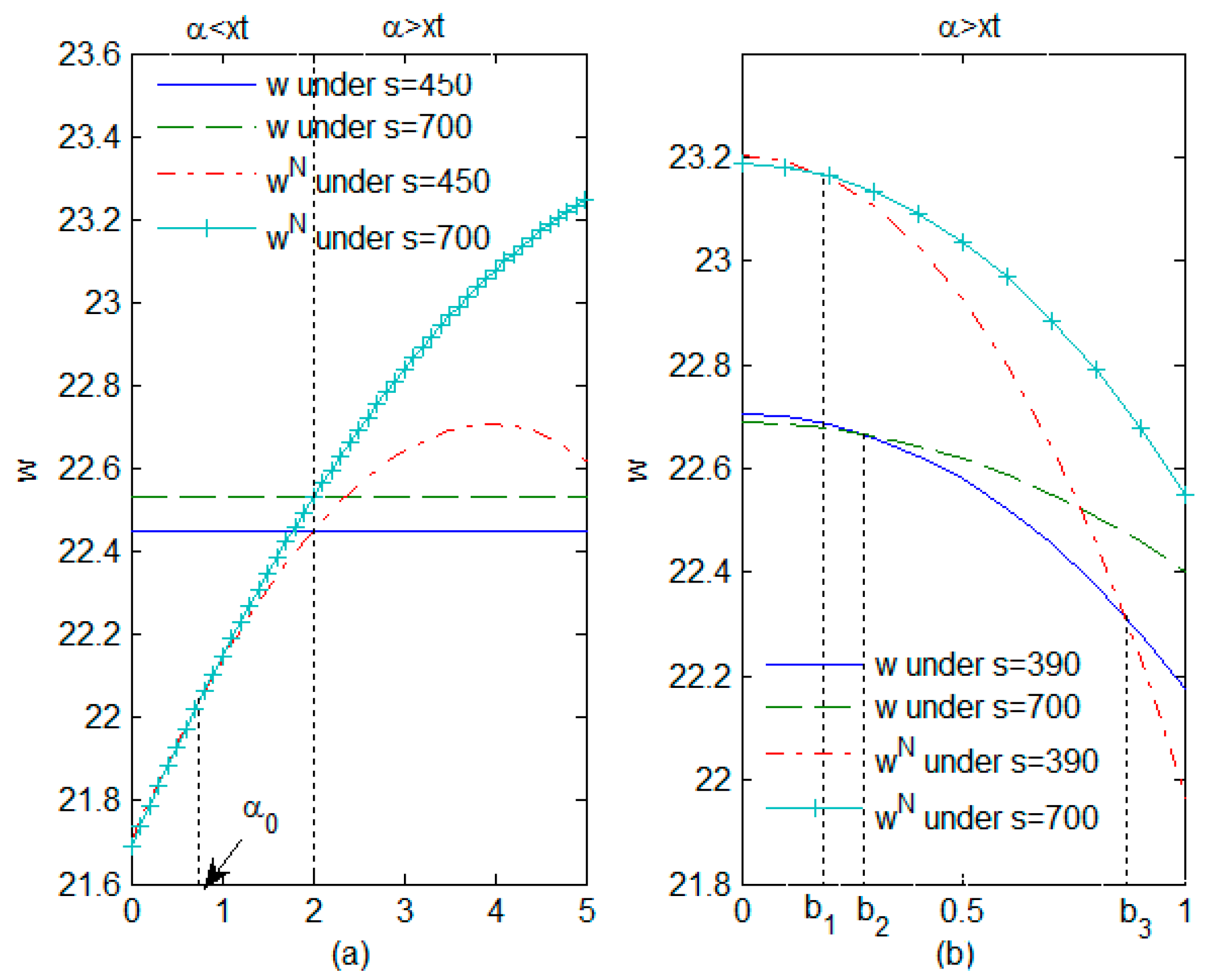
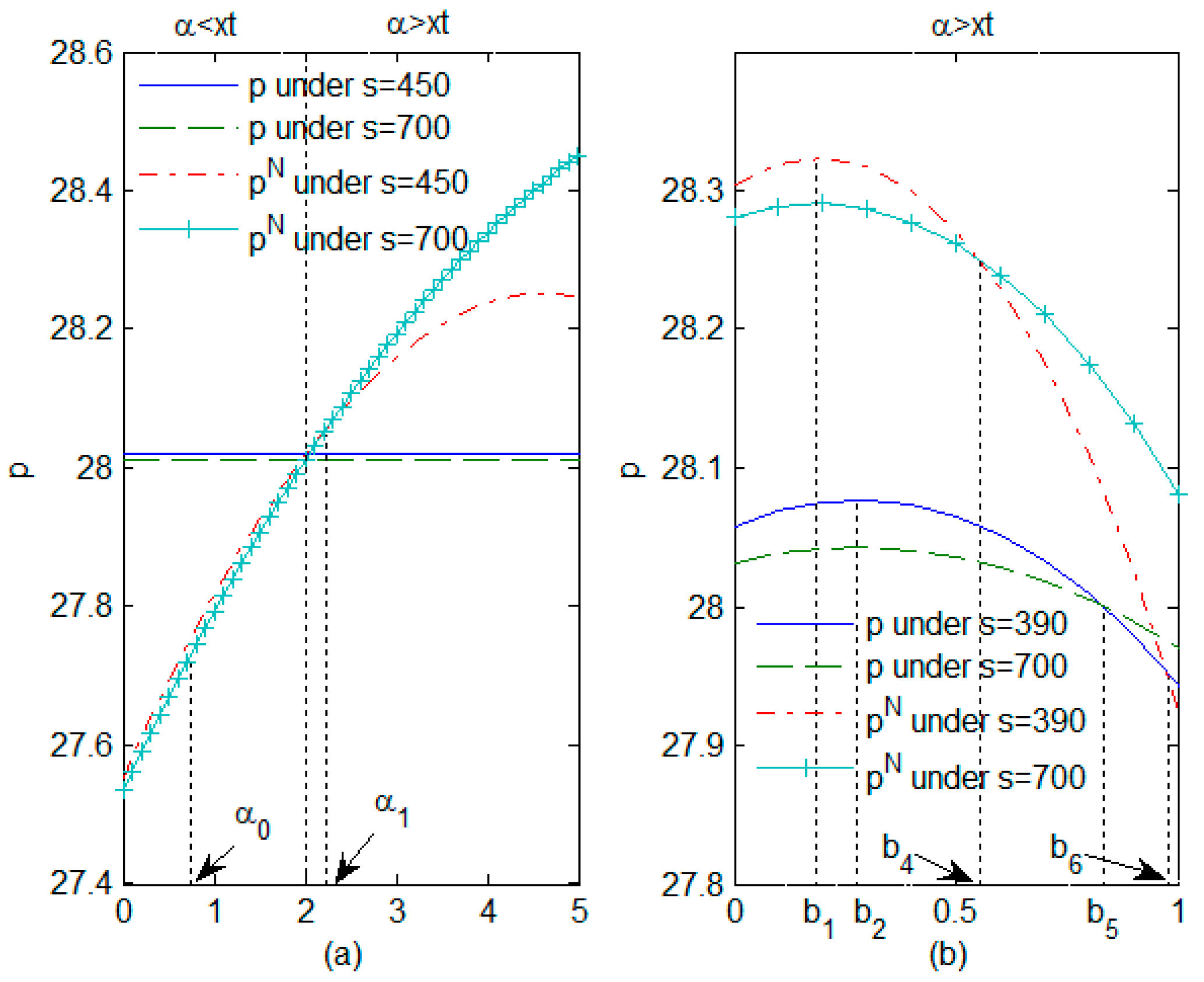
4.1. Impact of Carbon Tax per Unit of Product and Rate of Reduction in Carbon Emissions on Decision Variables

In this section, the first subfigure of Figure 1, Figure 2 and Figure 3 introduces the effect of $\alpha$ on the decision variables. The black dotted line represents the assumption that a non-uniform carbon tax policy and a uniform carbon tax policy have the same carbon tax per unit of product ($\alpha =xt$). Thus, the left side of the dotted line means $\alpha <xt$, while the right side of the dotted line shows $\alpha >xt$. Considering that $s_4\approx 438.62$ when $\alpha =5$, we have investigated the effect of α on the decision variables when $s=450$ and when $s=700$ in order to ensure that $s>s_4$. Similarly, we have analyzed the effect of $b$ on the decision variables when $s=390$ and when $s=700$ in the second subfigure of Figure 1, Figure 2 and Figure 3. The reason we chose this range of values for $s$ is that $s_4\approx 382.22$ when $b=1$. According to Corollary 1, we consider only $\alpha >{\alpha }_0=\frac{2\lambda }{ub(2-\theta )}$, $b\ge b_1=\frac{2\lambda }{u\alpha (2-\theta )}$ and $b\ge b_2=\frac{2\lambda }{uxt(2-\theta )}$ in order to ensure that the manufacturer prefers green innovations.

We set $b=0.75(b>\frac{2\lambda }{2a-u(2-\theta )(c+xt+\alpha )})$ in Figure 2a and $\alpha =3(\alpha >xt)$ in Figure 2b. Figure 2a shows that $e^N\le e$ when $\alpha \le xt$ (see the left part of dotted lines). Otherwise ($\alpha >xt$), $e^N>e$. This result confirms Corollary 6, which suggests that a high carbon tax per unit of product can increase the level of R&D effort when $b$ is relatively high. The production cost due to the high carbon tax per unit of product encourages the manufacturer’s enthusiasm for investment in green innovation investment and thus increases the level of R&D effort. Moreover, the level of R&D effort tends to increase when $s$ is low, which is consistent with Corollary 2. It is evident that as $s$ increases, the manufacturer’s incentive for R&D weakens due to the higher R&D costs involved. In the case in which a manufacturer opts for green innovation, as shown in Figure 2b, the level of R&D effort is positively correlated with $b$. High values for $b$ suggests greater returns from green innovation, denoted as $btE(D)$, which motivate the manufacturer to invest more in green innovation and increase the level of R&D effort to maximize profitability.

From Figure 3a, it is evident that the relationship between wholesale price and the carbon tax per unit of product followed an inverted U shape. The manufacturer’s total costs encompass R&D costs, production costs, and carbon tax expenditures. Referring to Figure 2, we observe that the level of R&D effort increases with the carbon tax per unit of product when $b>\frac{2\lambda }{2a-u(2-\theta )(c+xt+\alpha )}$. When the level of R&D effort is high, the rising costs of R&D lead to an increase in wholesale prices, whereas decreasing carbon tax expenditures contribute to a decline in wholesale prices. Whether wholesale prices increase or decrease depends on the relative magnitude of the increase in R&D costs compared to the decrease in carbon tax expenditures. If the increase in R&D costs outweighs the decrease in carbon tax expenditures, wholesale prices will rise. Conversely, wholesale prices will fall. In addition, it is intuitive that wholesale prices increase with the manufacturer’s cost, which is influenced by $s$, further confirming Corollary 2. Figure 3b illustrates that wholesale prices fall with an increase in $b$ when the manufacturer decides to invest in green innovation. The high $b$ enhances the manufacturer’s incentive for green innovation, leading to increased gains from green innovation and reduced carbon tax expenditures. Moreover, it is observed that $w^N\le w$ when $b\ge b_3$ and $s$ is relatively low, while $w^N>w$ when $b_2\le b<b_3$. This finding aligns with Corollary 6.

Similarly, the retail price also shows an inverted U-shaped relationship with the increase in $\alpha$. Figure 4a indicates the existence of ${\alpha }_1$ such that $\lambda =ub{\alpha }_1(2-\theta )/6$. The retail price declines as $s$ increases when ${\alpha }_0<\alpha \le {\alpha }_1$, while it increases with the increase in $s$ when $\alpha >{\alpha }_1$. This finding supports Corollary 2. Figure 4b reveals that the retail price decreases as $b$ increases when the manufacturer chooses to invest in green innovation. In an effect similar to that seen in Figure 3b, in the case in which $b$ is sufficiently high and $s$ is sufficiently low, we observe that $p^N\le p$. In addition, the retail price decreases as $s$ increases when $b_1<b\le b_4$ or $b_2<b\le b_5$. When $b>b_4$ or $b>b_5$, the retail price increases with $s$. Figure 2 illustrates that the level of R&D effort declines as $b$ increases, and lower level of R&D effort can lead to a decline in consumer demand. As a result, the retailer is more likely to opt for price reductions in order to increase consumer demand when $b$ is low and $s$ is high. In this scenario, an increase in $s$ will result in a decrease in retail prices.

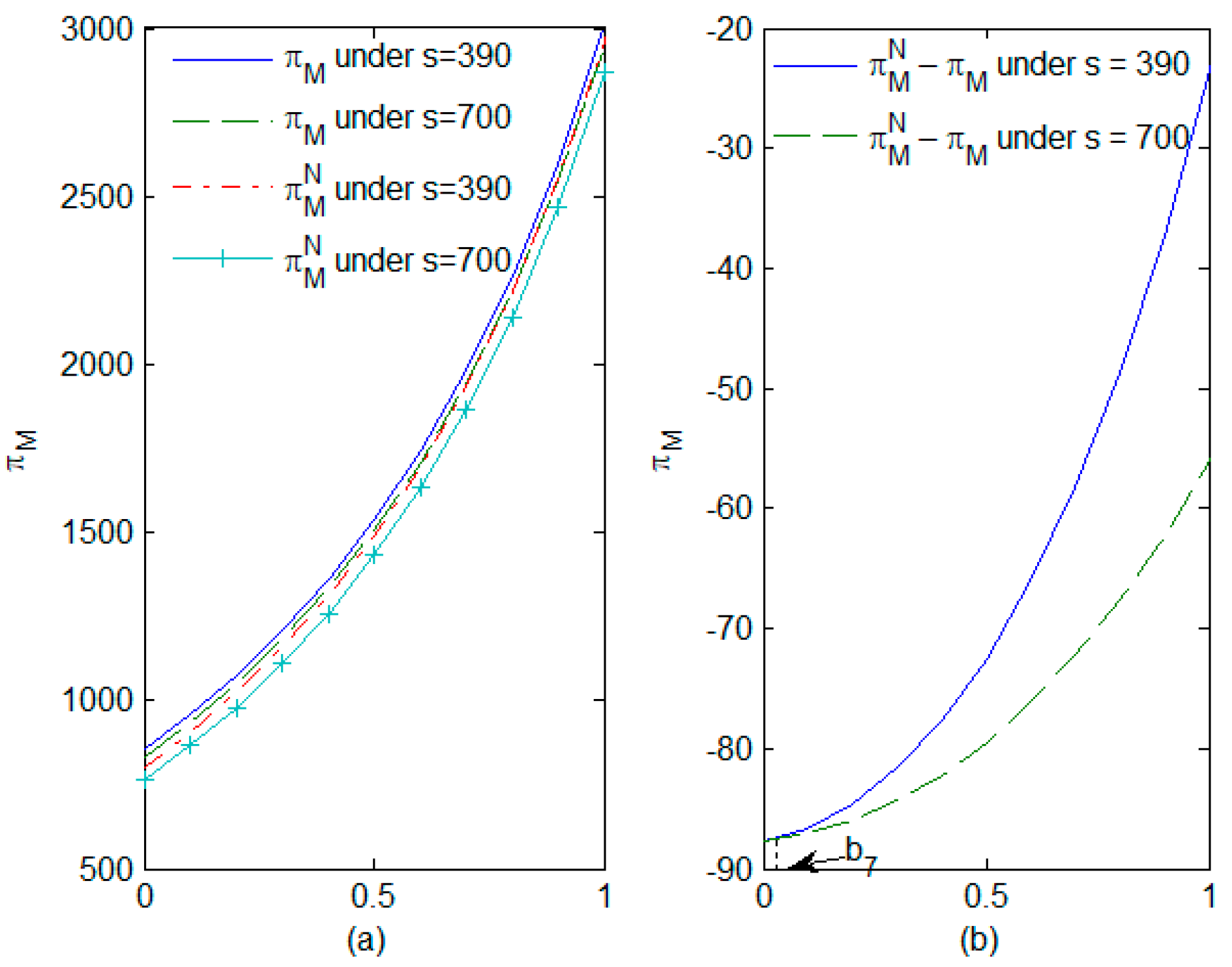
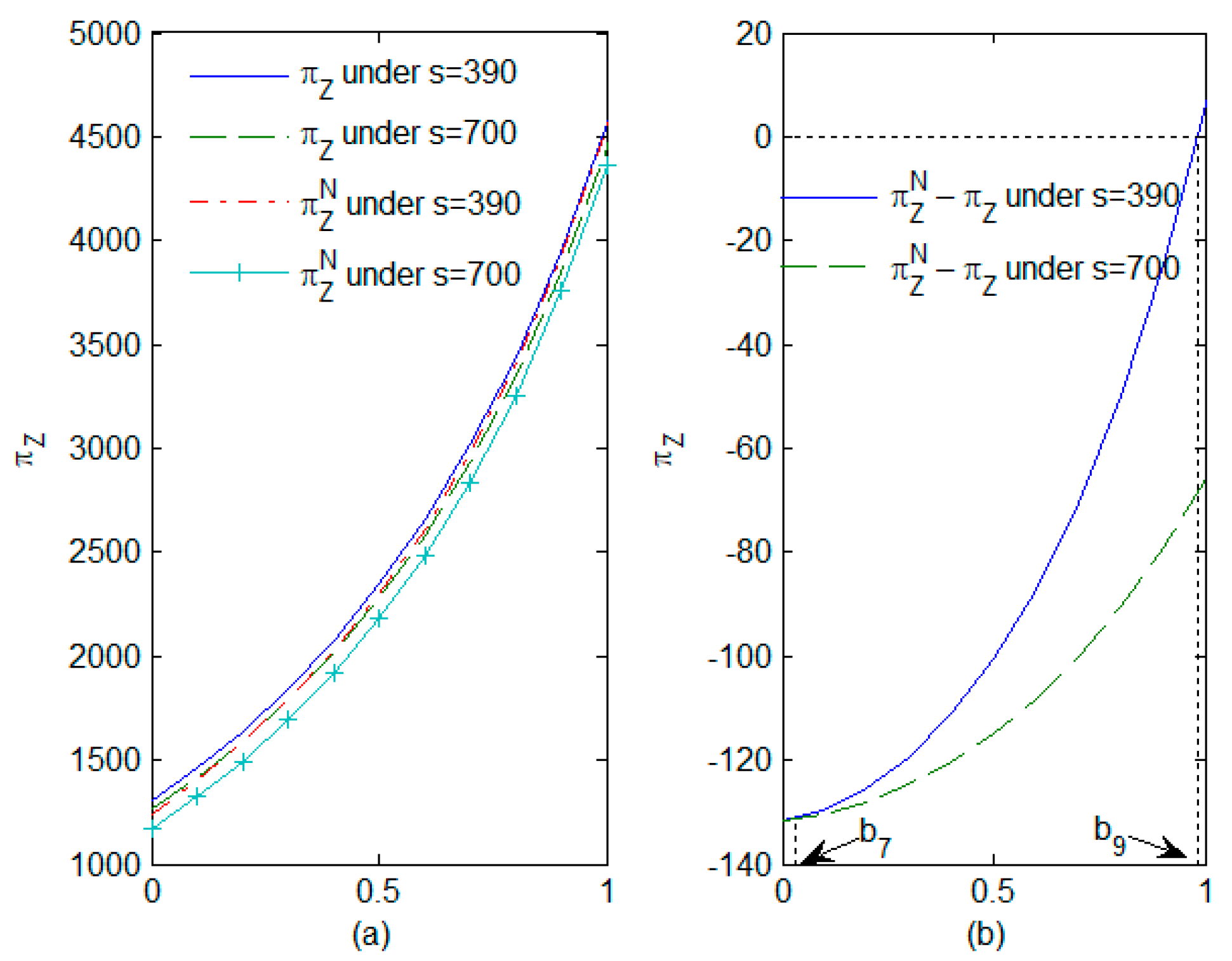
4.2. Impact of the Proportion of the Population with Green Preferences and the Rate of Reduction in Carbon Emissions on Expected Profits

In this section, Figure 5, Figure 6 and Figure 7 examine the impacts of $\theta$ and $b$ on the manufacturer’s expected profits, the retailer’s expected profits and the supply chain’s expected profits, respectively. According to Corollary 6, we consider only $b>b_7$, i.e., $2\lambda <b(4\lambda +2a-u(2-\theta )(c+(1-b)(\alpha +xt)))$.

Examining the first subfigure of Figure 5, Figure 6 and Figure 7, we observe that an increase in $\theta$ contributes to an increase in expected profit, thereby confirming Corollary 4. It is generally true that an increase in the number of consumers with green preferences, referred to as increased environmental awareness, can directly contribute to an overall increase in consumer demand for green products. The retailer and the manufacturer can benefit greatly from this increased demand. When $s$ is relatively low, ${\pi }_R^N>{\pi }_R$ in situations with high $\theta$. Low $s$ reduces the costs associated with green innovation and increases the probability of its successful implementation, and high $\theta$ increases consumer demand and reduces consumer price sensitivity. Consequently, the retailer makes more profit under a non-uniform carbon tax policy with a higher per-unit carbon tax than under a uniform carbon tax policy.

The second subfigure in Figure 5, Figure 6 and Figure 7 demonstrates that the carbon tax per unit of product diminishes the manufacturer’s expected profits. Moreover, under the conditions of low $s$ and high $b$, the retailer’s profits increase as the carbon tax per unit of product increases. Based on Corollary 2, a decrease in $s$ not only diminishes the cost associated with green innovation, but also results in increases R&D effort. Conversely, an increase in $b$ unequivocally amplifies the benefits of green innovation. Therefore, in a scenario characterized by low R&D costs and high benefits, the profitability of the retailer increases with consumer demand. When the growth in the retailer’s profits can compensate for the decline in the manufacturer’s profits, the overall profit of the supply chain also increases with $b$. This finding provides evidence supporting Corollary 6.

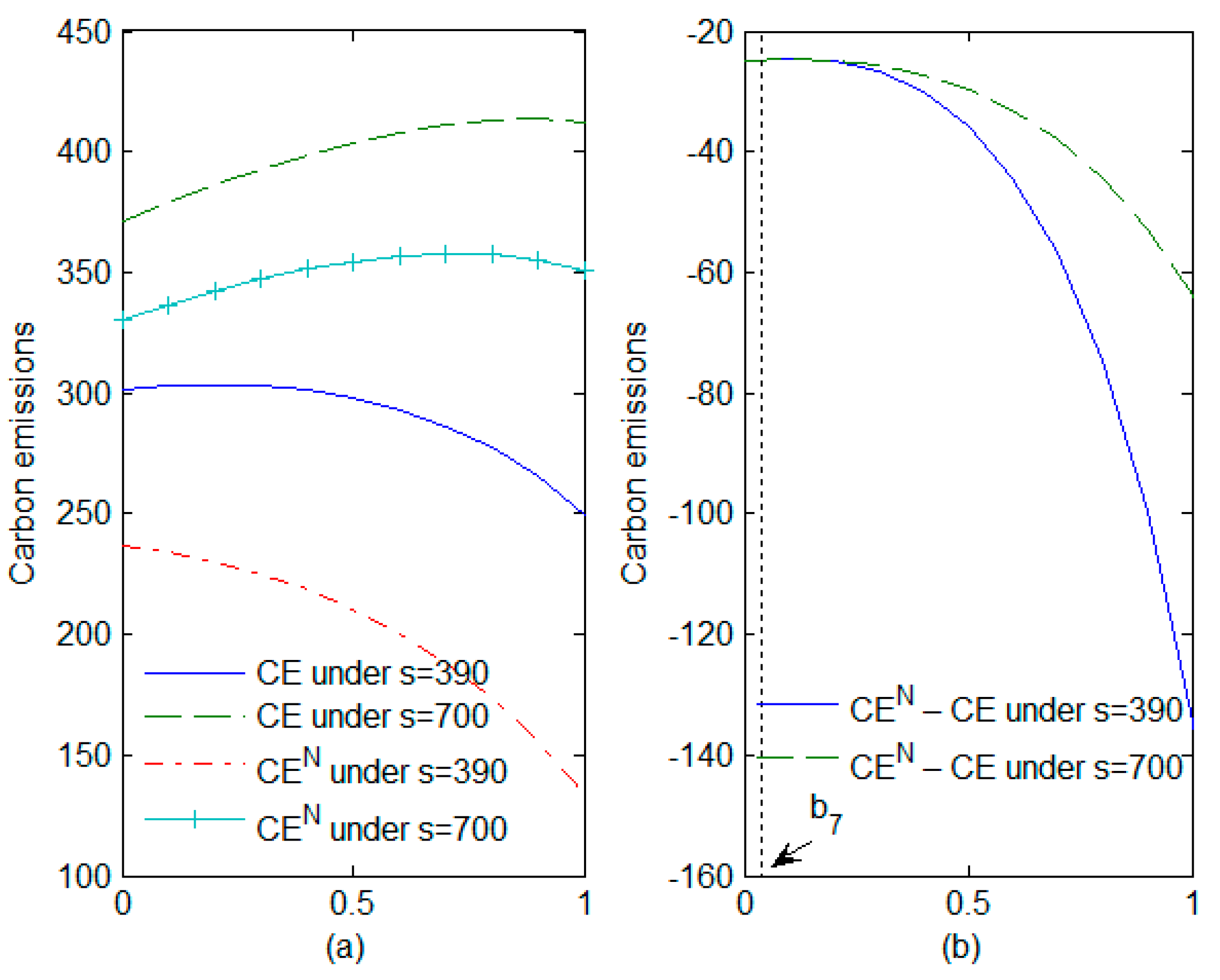
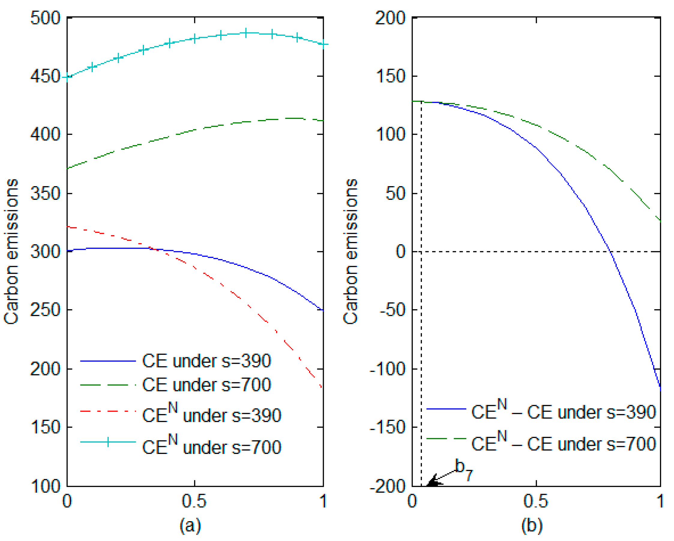
4.3. Impact of the Proportion of the Population with Green Preferences and the Rate of Reduction in Carbon Emissions on Carbon Emissions

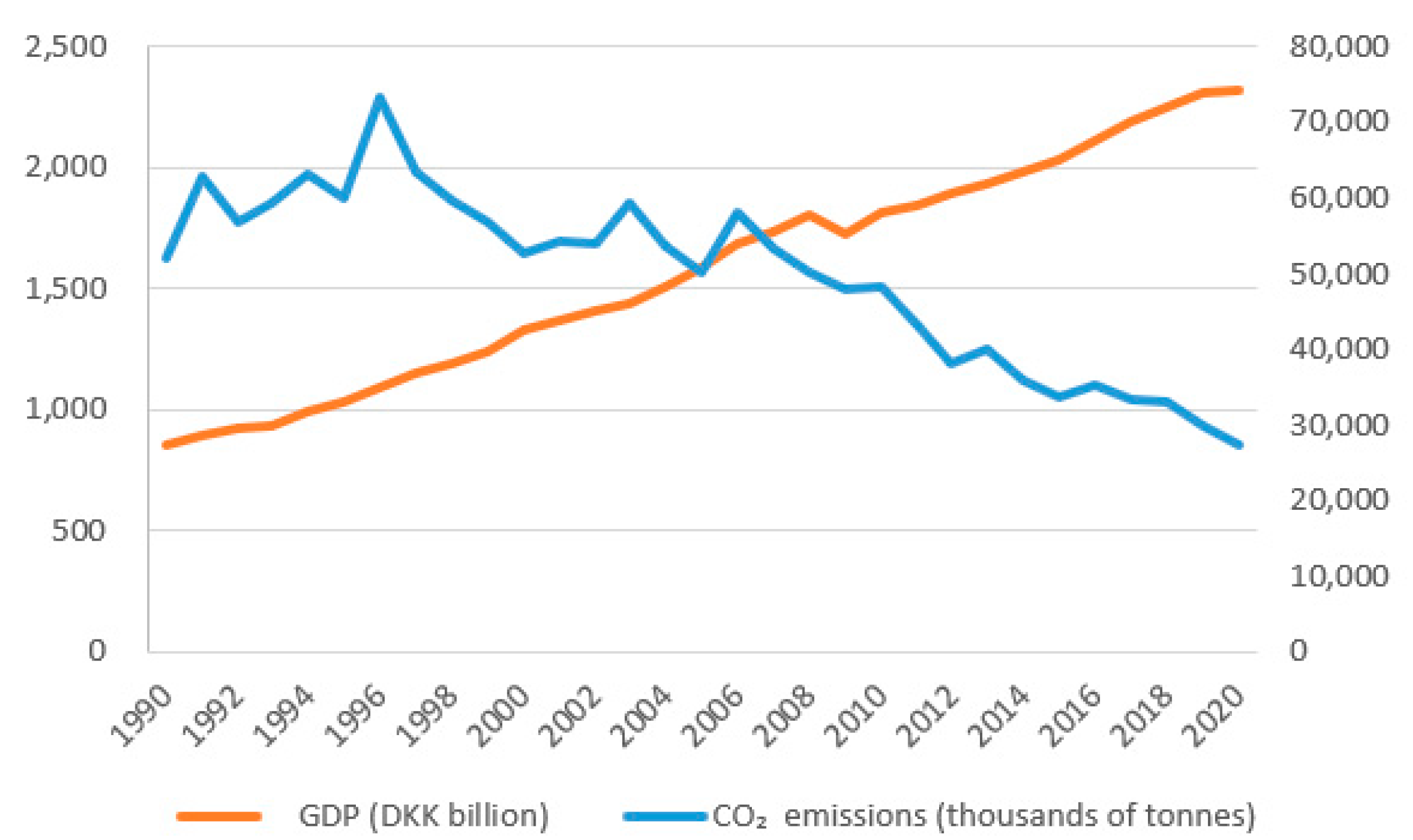
We set $t^{\prime }=m{t}_h+(1-m)t_l$ as the average carbon emissions per unit of product under the non-uniform carbon tax policy. Therefore, $C{E}^N=(1-e^{N}b)t^{\prime }{D}^N$ represents carbon emissions under a non-uniform carbon tax policy and $CE=(1-eb)tD$ represents carbon emissions under a uniform carbon tax policy. Figure 8 and Figure 9 analyze the impact of the proportion of the population with green preferences and the rate of reduction in carbon emissions on carbon emissions for two different scenarios: $t^{\prime }=t$ and $t^{\prime }>t$, respectively.

From Figure 8 and Figure 9, we observe an inverted U-shaped relationship between carbon emissions and $\theta$. This relationship can be explained by considering the interplay between consumer demand and R&D efforts. As $\theta$ increases, it increases the level of R&D effort and stimulates consumer demand. Higher consumer demand drives an increase in carbon emissions, while greater levels of R&D effort enhance the success of green innovations, leading to a reduction in carbon emissions. The relative strength of these two factors determines the overall trend in carbon emissions. If consumer demand has a more significant impact on carbon emissions, then as $\theta$ increases, carbon emissions are likely to rise. Conversely, if the level of R&D effort has a stronger effect, carbon emissions will tend to decrease. Notably, when $s$ is relatively high, the level of R&D efforts tends to decrease, making it more challenging for enterprises to reduce carbon emissions. Additionally, carbon emissions decrease as the carbon tax per unit of product increases when $t^{\prime }\le t$. However, when $t^{\prime }>t$, a high carbon tax per unit of product may have a negative impact on carbon emissions, particularly under conditions of low $s$. Therefore, the impact of carbon tax policies on the supply chain is contingent on the size of the carbon tax per unit of product. When the carbon tax policy increases the per-unit carbon tax, the profit of the supply chain and carbon emissions can reach a win-win situation under certain conditions.

Based on the perspective of enterprise development, it is crucial for supply-chain members to collaborate synergistically to increase the proportion of consumers with green preferences. From the standpoint of green and sustainable development, the government should adopt a comprehensive and integrated plan when formulating carbon tax policies. Such a plan should consider the input-output ratio of enterprises’ green innovation. It is important to strike a balance in which the benefits of green innovation outweigh the associated costs. If the costs of implementing green innovation are high and the benefits are low, the effectiveness of the carbon tax policy could be significantly reduced and such policies may even have short-term negative impacts. In summary, supply-chain members should coordinate their efforts and allocate responsibilities effectively. Low-$s$ firms, which have a comparative advantage in implementing green practices, should take the lead in expanding the proportion of consumers with green preferences. On the other hand, high-$s$ firms should focus on reducing the costs associated with green innovation. By dividing labor in this manner, each firm can leverage its strengths to contribute to the overall sustainability of the supply chain. Furthermore, enterprises that have already developed effective carbon-reduction technologies should share their knowledge and technologies with others. This collaboration can help increase the overall rate of carbon reduction in society, promoting a more sustainable environment and benefiting the entire supply chain.

5. Case Study

A carbon tax is a tax imposed on the consumption or use of fossil fuels with the aim of mitigating greenhouse-gas emissions. Denmark was one of the first countries to implement a carbon tax policy. At present, carbon tax policy is undoubtedly an important tool for the development of a low-carbon economy in Denmark.

5.1. Implementation Background

In response to the oil crisis of the early 1970s, Denmark introduced a general energy tax on households and non-VAT businesses in 1977. Since the 1990s, driven by heightened environmental consciousness and a steadfast pursuit of energy self-sufficiency, Denmark has formally instituted a nationwide carbon-taxation scheme for all sectors of the economy. A carbon dioxide tax and a sulfur dioxide tax were created. Notably, the energy-consumption tax comprises various autonomous sub-taxes, which uphold the stability of the carbon tax policy framework.

5.2. Implementation Plan

In Denmark, the government has employed a revenue-allocation strategy within the framework of the carbon tax policy to promote public acceptance of the policy. A portion of the carbon tax revenue is channeled towards subsidizing enterprises, thereby incentivizing their active engagement in energy-efficiency initiatives. Furthermore, Denmark actively supports domestic businesses by offering differentiated carbon tax rebates based on types of energy utilization such as heating, production, and lighting. To ensure a concerted effort towards reducing carbon emissions, the Danish Parliament established a noteworthy objective in 1990, aiming for a 20 percent decrease in domestic CO₂ emissions by 2005 relative to the 1988 baseline. Aligning with international commitments like the Tokyo Protocol and EU agreements, Denmark subsequently revised its carbon-emission reduction target to 21 percent below 1990 levels, to be achieved within 2008–2012. For a comprehensive overview of the implementation of Danish carbon tax policy, please refer to

Table 2. Implementation of carbon tax policies in Denmark.

Carbon Tax Policy	Year	Status of Implementation
General energy tax	1977	The general energy tax initially targeted petroleum products and electricity. The energy tax was imposed on coal in 1982. Subsequently, in 1997, natural gas was also included under the energy-tax framework. In 2013, the electricity tax was abolished.
Carbon dioxide tax	1992	The carbon dioxide tax is levied on the energy consumed by different sectors. The current tax system is designed to differentiate rates based on the carbon dioxide content of various fuels. The intention is to ensure that the price of the tax for different types of energy is approximately equivalent to a tax of DKK 100 per ton of carbon dioxide emitted.
Sulfur dioxide tax	1996	There are two tax methods available to taxable enterprises. The first method is a product tax, which is levied based on the sulfur content of the taxable fuel. The tax rate for the product tax is set at DKK 20 per kilogram of sulfur. The second method is an emissions tax, which is imposed based on the actual emissions of sulfur dioxide. The tax rate for the emissions tax is DKK 10 per kilogram of sulfur dioxide emitted.

.

5.3. Implementation Effect

According to Figure 10, Denmark has achieved remarkable results in reducing carbon dioxide emissions and simultaneously experiencing steady economic growth. Between 1990 and 2020, Denmark’s carbon dioxide emissions decreased by approximately 50 percent. During the same period, Denmark’s GDP increased by 2.7 times, reaching approximately $355.2 billion in 2020. This data demonstrates that Denmark has been successful in striking a balance between achieving environmental objectives and garnering acceptance for the carbon tax policy among all stakeholders. Denmark’s experience serves as a testament to the fact that a well-designed carbon tax system can contribute to both environmental protection and sustained economic development. It showcases the development of a Danish model that harmonizes economic growth with ecological conservation. By building on its existing energy tax system and integrating complementary taxes, Denmark has established a green tax system that has yielded positive outcomes. This experience positions Denmark as a valuable source of knowledge about utilizing tax instruments to protect the environment and foster sustainable development.

Over the long term, the implementation of the Danish carbon tax has effectively curbed carbon emissions while maintaining economic stability. In the short term, however, the introduction of the carbon tax initially contributed to increased carbon emissions and negatively impacted economic development. The findings of this study demonstrate that a high carbon tax per unit of product consistently reduces manufacturers’ profits. Nevertheless, when green innovation yields significant benefits at relatively low costs, retailers’ profits will increase with the carbon tax per unit of product, thereby further increasing the profitability of the supply chain. Simultaneously, it is crucial to note that a high carbon tax per unit of product does not invariably ensure a reduction in carbon emissions. When the benefits derived from green innovation are relatively limited, a high carbon tax per unit of product may inadvertently lead to greater carbon emissions, particularly in situations in which the carbon emissions per unit of product are relatively high. Due to the long payback periods and substantial investment required for the development of green innovations and the production of green products, it is expected that in the short term, supply-chain profits may decline as a result of the reduction in the manufacturers’ profits. This situation can have adverse effects on national economic development and lead to higher carbon emissions. However, in the long term, with an increased proportion of consumers with green preferences, there is an increasing demand for green products, which boosts the manufacturer’s profits. The higher profits then contribute to increased investments in green innovation, thereby promoting the development of green-innovation technologies and allowing the supply chain to benefit from economies of scale. Ultimately, the virtuous economic cycle enhances economic development and reduces carbon emissions. These findings are consistent with the reality seen in Denmark.

6. Conclusions

This paper investigates a green supply chain consisting of a manufacturer and a retailer under the different types of carbon tax policy. For each model, we obtain the optimal level of R&D effort and pricing decisions and examine the impact of the proportion of the population with green preferences and the rate of reduction in carbon emissions on expected profits and carbon emissions. The main findings of this paper can be summarized as follows.

(1)

Carbon tax policies significantly influence supply-chain decisions by affecting the carbon tax per unit of product. Regardless of whether the carbon tax policy is uniform or non-uniform, an increase in the carbon tax per unit of product leads to a higher level of R&D effort. However, wholesale and retail prices exhibit an inverted U-shaped relationship with the carbon tax per unit of product. An increase in R&D costs and in the proportion of green-preferring consumers will raise wholesale prices but can reduce retail prices under certain conditions. The gains derived from green innovation result in a reduction in both wholesale and retail prices. Furthermore, an increase in the carbon tax per unit of product correspondingly contributes to a decrease in wholesale and retail prices when the benefits of green innovation are sufficiently high.

(2)

Consumers’ green preferences positively impact the expected profits of supply chains and have an inverted U-shaped relationship with carbon emissions. In situations in which the proportion of consumers with green preference is relatively high, a high carbon tax per unit of product can result in increased profits for the retailer and even reduce the profits of the supply chain. Conversely, when the proportion of consumers with green preferences is relatively low, policies involving a high carbon tax per unit of product might inadvertently lead to an increase in carbon emissions, particularly in scenarios characterized by low R&D costs. Meanwhile, manufacturers with high R&D costs at the same level of green preference have higher carbon emissions.

(3)

A high carbon tax per unit of product will always reduce the manufacturer’s profits, but in the case of high R&D returns and low innovation costs, the retailer’s profit may increase as well. When the gain in profits for a retailer is greater than the loss in profits for a manufacturer, the overall profits of the supply chain will increase with the carbon tax per unit of product. Additionally, when the benefits associated with green innovation are relatively low, a high carbon tax per unit of product can contribute to increased carbon emissions, particularly in situations in which the carbon emissions per unit of product are relatively high.

Therefore, manufacturers should concentrate on reducing R&D costs to produce low-carbon products that satisfy both consumer demand and requirements for sustainable development in the context of green development. Supply-chain members should collaborate to cultivate consumers’ green preferences. When the ratio of R&D output to input is relatively low, the government should reduce the carbon tax per unit of product to reduce the cost pressure on supply chains and also reduce carbon emissions. However, a higher carbon tax per unit of product can result in a win-win situation when the output-to-input ratio is relatively high.

This research can be extended in several directions to explore additional aspects in the future. This paper considers only the impact of consumers’ green preference behavior on supply chain members’ optimal decision-making and on carbon emissions under different carbon tax policies. We can further study the impact of consumers’ green preferences on optimal decision-making in the supply chain in a dual-channel green supply chain. In addition, carbon tax subsidy policies may also be considered.

References

1. Mitra, S.; Datta, P.P. Adoption of green supply chain management practices and their impact on performance: An exploratory study of Indian manufacturing firms. Int. J. Prod. Res. 2014, 52, 2085–2107. [Google Scholar] [CrossRef]
2. Wen, X.; Cheng, H.; Cai, J.; Lu, C. Govrnment subside policies and effect analysis in green supply chain. Chin. J. Manag. 2018, 15, 625–632. [Google Scholar]
3. Liu, G.; Yang, T.; Zhang, X. Pricing of green supply chain and decisions on product green degree considering green preference and sales effort. J. Beijing Jiaotong Univ. (Soc. Sci. Ed.) 2019, 18, 115–126. [Google Scholar] [CrossRef]
4. Fussler, C.; James, P. Driving Eco-Innovation: A Breakthrough Discipline for Innovation and Sustainability; Pitman Publishing: London, UK; Washington, DC, USA, 1996; pp. 68–74. ISBN 978-0-273-62207-9. [Google Scholar]
5. Wang, W.; Zhang, R. Research on financing strategies for green product suppliers under government subsidies—Green credit VS prepayment. J. Syst. Manag. 2023, accepted. [Google Scholar]
6. Liu, S.; Zhang, Y. Greenhouse gas emissions reduction: A theoretical framework and global solution. Econ. Res. J. 2009, 44, 4–13. [Google Scholar]
7. Zhang, J.; Wang, K.; Zhang, Y. Carbon emission abatement performance of carbon emissions trading scheme—Based on the intermediary effect of low-carbon technology innovation. Soft Sci. 2022, 36, 102–108. [Google Scholar] [CrossRef]
8. Zhou, D.; Cai, X.; Zhang, D.; Zhang, Y. Carbon tax policy simulation based on CGE model: A case study of Guangdong province. Clim. Change Res. 2020, 16, 516–525. [Google Scholar]
9. Ghosh, D.; Shah, J. Supply chain analysis under green sensitive consumer demand and cost sharing contract. Int. J. Prod. Econ. 2015, 164, 319–329. [Google Scholar] [CrossRef]
10. Li, B.; Zhu, M.; Jiang, Y.; Li, Z. Pricing policies of a competitive dual-channel green supply chain. J. Clean. Prod. 2016, 112, 2029–2042. [Google Scholar] [CrossRef]
11. Gao, J.; Han, H.; Hou, L. Decision-making in closed-loop supply chain with dominant retailer considering products’ green degree and sales effort. Manag. Rev. 2015, 27, 187–196. [Google Scholar] [CrossRef]
12. Zhang, C.-T.; Liu, L.-P. Research on coordination mechanism in three-level green supply chain under non-cooperative game. Appl. Math. Model. 2013, 37, 3369–3379. [Google Scholar] [CrossRef]
13. Zhou, Y.; Hu, J.; Liu, J. Decision analysis of a dual channel green supply chain considering the fairness concern. Ind. Eng. Manag. 2020, 25, 9–19. [Google Scholar] [CrossRef]
14. Jiang, S.; Li, S.; Wang, H. Pricing decision of green supply chain considering risk aversion. Syst. Eng. 2016, 34, 94–100. [Google Scholar]
15. Liu, P.; Yi, S. Pricing policies of green supply chain considering targeted advertising and product green degree in the big data environment. J. Clean. Prod. 2017, 164, 1614–1622. [Google Scholar] [CrossRef]
16. Liu, S.S.; Hua, G.; Ma, B.J.; Cheng, T.C.E. Competition between green and non-green products in the blockchain era. Int. J. Prod. Econ. 2023, 264, 108970. [Google Scholar] [CrossRef]
17. Yang, S.; Xiao, D. Channel choice and coordination of two-stage low-carbon supply chain. Soft Sci. 2017, 31, 92–98. [Google Scholar] [CrossRef]
18. Zhou, Y.; Hu, F.; Zhou, Z. Study on joint contract coordination to promote green product demand under the retailer-dominance. J. Ind. Eng. Eng. Manag. 2020, 34, 194–204. [Google Scholar] [CrossRef]
19. Lin, D. Accelerability vs. scalability: R&D investment under financial constraints and competition. Manag. Sci. 2023, 69, 4078–4107. [Google Scholar] [CrossRef]
20. Zhu, W.; He, Y. Green product design in supply chains under competition. Eur. J. Oper. Res. 2017, 258, 165–180. [Google Scholar] [CrossRef]
21. Benjaafar, S.; Li, Y.; Daskin, M. Carbon footprint and the management of supply chains: Insights from simple models. IEEE Trans. Autom. Sci. Eng. 2013, 10, 99–116. [Google Scholar] [CrossRef]
22. Yang, H.; Luo, J. Emission reduction in a supply chain with carbon tax policy. Syst. Eng.-Theory Pract. 2016, 36, 3092–3102. [Google Scholar]
23. Ma, Q.; Song, H.; Chen, G. Research on product pricing and production decision-making under the supply chain environment considering the carbon-trading mechanism. Chin. J. Manag. Sci. 2014, 22, 37–46. [Google Scholar] [CrossRef]
24. Cao, X.; Wu, X. The Collaborative strategy for carbon reduction technology innovation on dual-channel supply chain under the carbon tax policy. J. Cent. China Norm. Univ. (Nat. Sci.) 2020, 54, 898–909. [Google Scholar] [CrossRef]
25. Xiong, Z.; Zhang, P.; Guo, N. Impact of carbon tax and consumers’ environmental awareness on carbon emissions in supply chains. Syst. Eng.-Theory Pract. 2014, 34, 2245–2252. [Google Scholar]
26. Xu, C.; Wang, C.; Huang, R. Impacts of horizontal integration on social welfare under the interaction of carbon tax and green subsidies. Int. J. Prod. Econ. 2020, 222, 107506. [Google Scholar] [CrossRef]
27. Yu, W.; Wang, Y.; Feng, W.; Bao, L.; Han, R. Low carbon strategy analysis with two competing supply chain considering carbon taxation. Comput. Ind. Eng. 2022, 169, 108203. [Google Scholar] [CrossRef]
28. Zhou, Y.; Hu, F.; Zhou, Z. Pricing decisions and social welfare in a supply chain with multiple competing retailers and carbon tax policy. J. Clean. Prod. 2018, 190, 752–777. [Google Scholar] [CrossRef]
29. Jaber, M.Y.; Glock, C.H.; El Saadany, A.M.A. Supply chain coordination with emissions reduction incentives. Int. J. Prod. Res. 2013, 51, 69–82. [Google Scholar] [CrossRef]
30. Diao, X.; Zeng, Z.; Sun, C. Research on coordination of supply chain with two products based on mix carbon policy. Chin. J. Manag. Sci. 2021, 29, 149–159. [Google Scholar] [CrossRef]
31. Ghosh, A. Optimization of a production-inventory model under two different carbon policies and proposal of a hybrid carbon policy under random demand. Int. J. Sustain. Eng. 2021, 14, 280–292. [Google Scholar] [CrossRef]
32. Zhao, L.; Jin, S.; Jiang, H. Investigation of complex dynamics and chaos control of the duopoly supply chain under the mixed carbon policy. Chaos Solitons Fractals 2022, 164, 112492. [Google Scholar] [CrossRef]
33. Zhu, C.; Ma, J.; Li, J. Joint emission reduction decisions and Its optimization under hybrid carbon regulations. J. Syst. Manag. 2023, accepted. [Google Scholar]
34. Zhu, C.; Ma, J. Optimal decisions in two-echelon supply chain under hybrid carbon regulations: The perspective of inner carbon trading. Comput. Ind. Eng. 2022, 173, 108699. [Google Scholar] [CrossRef]
35. Li, X.; Han, R. Impact of government policy on supply chain enterprises decisions under the low-carbon economy. Sci. Technol. Manag. Res. 2016, 36, 240–245. [Google Scholar]
36. Chen, W.; Hu, Z.-H. Using evolutionary game theory to study governments and manufacturers’ behavioral strategies under various carbon taxes and subsidies. J. Clean. Prod. 2018, 201, 123–141. [Google Scholar] [CrossRef]
37. Guo, J.; Huang, R. A carbon tax or a subsidy? Policy choice when a green firm competes with a high carbon emitter. Environ. Sci. Pollut. Res. 2022, 29, 12845–12852. [Google Scholar] [CrossRef]
38. Meng, W. Comparation of subsidy and cooperation policy based on emission reduction R & D. Syst. Eng. 2010, 28, 123–126. [Google Scholar]
39. Vaughan, D.; Skerritt, D.J.; Duckworth, J.; Sumaila, U.R.; Duffy, M. Revisiting Fuel Tax Concessions (FTCs): The economic implications of fuel subsidies for the commercial fishing fleet of the United Kingdom. Mar. Policy 2023, 155, 105763. [Google Scholar] [CrossRef]
40. Qiu, R.; Xu, J.; Xie, H.; Zeng, Z.; Lv, C. Carbon tax incentive policy towards air passenger transport carbon emissions reduction. Transp. Res. Part D: Transp. Environ. 2020, 85, 102441. [Google Scholar] [CrossRef]
41. Zhang, W.; Lee, H.-H. Investment strategies for sourcing a new technology in the presence of a mature technology. Manag. Sci. 2022, 68, 4631–4644. [Google Scholar] [CrossRef]
42. He, Y.; Chen, Z.; Liao, N. The impact mechanism of government subsidy approach on manufacturer’s decision—Making in green supply chain. Chin. J. Manag. Sci. 2022, 30, 87–98. [Google Scholar] [CrossRef]
43. Deng, L.; Liu, Z. One-period pricing strategy of ‘Money Doctors’ under cumulative prospect theory. Port. Econ. J. 2017, 16, 113–144. [Google Scholar] [CrossRef]
Figure 1. The sequence of events.
Mathematics 11 04631 g001
Figure 2. Effect of α and b on the level of R&D effort: (a) the impact of α; (b) the impact of b.
Mathematics 11 04631 g002
Figure 3. Effect of α and b on the wholesale price: (a) the impact of α; (b) the impact of b.
Mathematics 11 04631 g003
Figure 4. Effect of α and b on the retail price: (a) the impact of α; (b) the impact of b.
Mathematics 11 04631 g004
Figure 5. Impact of θ and b on the manufacturer’s expected profits: (a) the impact of θ; (b) the impact of b.
Mathematics 11 04631 g005
Figure 6. Impact of θ and b on the retailer’s expected profits: (a) the impact of θ; (b) the impact of b.
Mathematics 11 04631 g006
Figure 7. Impact of θ and b on the supply chain’s expected profits: (a) the impact of θ; (b) the impact of b.
Mathematics 11 04631 g007
Figure 8. Impact of θ and b on carbon emissions when t′ = t: (a) the impact of θ; (b) the impact of b.
Mathematics 11 04631 g008
Figure 9. Impact of θ and b on carbon emissions when t′ > t: (a) the impact of θ; (b) the impact of b.
Mathematics 11 04631 g009
Figure 10. Total CO2 emissions and GDP in Denmark from 1990 to 2020.
Mathematics 11 04631 g010