1. Introduction
Interest in quadrotor systems has been increasing continuously. This is because of their versatility and potential for various applications. Quadrotors are unmanned aerial vehicles that offer unique advantages in terms of mobility and access to challenging locations, making them suitable for aerial surveillance, structural inspection, delivery services, and more [
1,
2,
3,
4]. However, controlling a quadrotor presents significant challenges in terms of ensuring stability and achieving precise control. Modeling a quadrotor is crucial for understanding the system dynamics and developing control algorithms. It allows us to comprehend the interaction between the motion along each axis and the control inputs. Typically, quadrotor modeling is divided into two parts: rotational motion and translational motion. Rotational motion is controlled via the roll, pitch, and yaw axes, whereas translational motion is controlled via the
x,
y, and
z axes. Quadrotor modeling is performed using kinematic and dynamic principles. Kinematic modeling derives equations that represent the position and velocity, whereas dynamic modeling describes the quadrotor’s motion equations. These models enable mathematical expression of the relationship between the state and control inputs of a quadrotor.
Quadrotors are generally underactuated systems with four actuators and six degrees of freedom. This means that some degrees of freedom of the quadrotor are not directly controlled but are influenced by other degrees of freedom. Therefore, to control a quadrotor, we must fix four degrees of freedom and directly derive control signals for the remaining two degrees of freedom. In this study, we employed a method that fixed the
x,
y, and
z axes and yaw angle and derived control equations for the roll and pitch angles [
5]. This involved analyzing the quadrotor motion equations and their relationship with the control inputs to derive suitable control algorithms. This modeling approach provides a foundation for addressing the quadrotor control problem and plays a crucial role in the application of the proposed control method. Furthermore, it enables improved stability and performance in quadrotor control.
One of the commonly used control methods for quadrotors is proportional–integral–derivative (PID) control. PID control is known for its simplicity and ease of design; therefore, it is widely used not only in quadrotors but also for controlling various other devices [
6,
7]. However, PID control is highly susceptible to external disturbances and does not offer a robust response. Sliding mode control (SMC) has been developed to overcome these limitations. SMC provides robustness against external disturbances and serves as a prominent nonlinear control method that complements the limitations of PID control. Consequently, SMC is frequently employed in quadrotor control, where a robust control is required [
8,
9,
10,
11]. SMC offers robustness against disturbances and uncertainties; however, by Lyapunov stability analysis, traditional SMC exhibits a phenomenon known as chattering. Because of discontinuous reaching law term, chattering refers to the high-frequency switching of control inputs and occurs during the transition from the reaching phase to sliding phase in SMC. This chattering phenomenon can lead to undesirable effects such as mechanical stress and instability. In addition, because the quadrotor is an underactuated system, there are signals that must be additionally designed to control all states of system, so the chattering effect causes serious problems in the quadrotor system. To address this issue, a control method called second-order sliding mode control (SOSMC) has been proposed [
12,
13,
14,
15,
16]. SOSMC operates on principles similar to those of SMC but it is highly effective in reducing chattering and improving control performance. Consequently, numerous studies have investigated the application of SOSMC in quadrotor control [
17,
18]. Replacing the conventional Lyapunov stability evaluation method, strict Lyapunov functions guarantee convergence within a finite time, offer a prediction of the convergence time, and confirm the robustness of flight control performance or ultimate boundedness for a broader range of disturbances than the conventional method.
Although SOSMC has shown promising results in reducing chattering, improvements can still be made in terms of stability and control effectiveness. Therefore, research was also conducted to enhance SOSMC [
19]. To address this issue, we developed an improved control method called advanced second-order sliding mode control (ASOSMC). The ASOSMC combines the advantages of SOSMC with the incorporation of a powerful term to achieve strict Lyapunov stability, adaptive control laws, and additional enhancements for superior stability and performance in quadrotor control. The additional term is separated from the signum function, making it robust to the effects of chattering. This allows for the application of higher gain values compared to traditional SOSMC, enabling more stable maneuvering than SOSMC. Typically, the stability of SMC is evaluated using the Lyapunov stability [
20,
21]. However, for SOSMC, which involves an additional dimension in the reaching law, proving its stability using conventional Lyapunov functions becomes challenging. Therefore, in this study, we introduced strict Lyapunov stability instead of the conventional Lyapunov stability to establish the stability of the system [
22,
23]. This study focused on the ASOSMC approach and investigated its potential for enhancing the stability and control performance of quadrotor systems. The limitations of traditional SMC and the improvements introduced by SOSMC are discussed. In addition, the advanced features of the ASOSMC, such as strict Lyapunov stability, adaptive control laws, and a reduction in chattering, are addressed comprehensively. Since ASOSMC is proposed to have the same control input dimensions as SOSMC, the stability evaluation of the presented control law can be analyzed by the strict Lyapunov stability evaluation method. Through simulation experiments and comparative analysis, the superior performance of the ASOSMC was demonstrated by comparing it with traditional SMC and SOSMC. The main contributions of this study can be summarized as follows:
ASOSMC is designed employing a novel form of reaching law, allowing the quadrotor to track stably by introducing an additional robust term.
To stabilize the subsystems of the quadrotor closed-loop system, stability is ensured using strict Lyapunov functions.
By transforming the three vectors resulting from the addition of an extra robust term into two vector expressions, we applied the principle of a strict Lyapunov function, proving stability in a manner similar to conventional SOSMC.
The proposed theoretical results were demonstrated to be effective by simulating external disturbances and comparing the outcomes with those obtained using alternative methods.
In
Section 2, we introduce the basic modeling of the Parrot Mambo quadrotor, used in this study, and explain the methods for operating the quadrotor. We also derive equations for generating the remaining roll and pitch angles by exploiting the fact that the quadrotor is an underactuated system. In
Section 3, we discuss SMC, which is essential for system control, and derive the sliding surface, which is a key component of SMC control. In
Section 4, the newly proposed ASOSMC system is presented based on the sliding surface derived in
Section 3. Furthermore, the stability of the system is demonstrated using strict Lyapunov stability. In
Section 5, the performance of the ASOSMC is evaluated via simulation experiments. Finally, in the conclusion, we summarize the findings of this study. The results of this study contribute to the advancement of quadrotor control methodologies and emphasize the value of achieving more stable and precise quadrotor control in practical applications. By utilizing the capabilities of the ASOSMC, the limitations of existing control methods can be overcome and more stable and accurate quadrotor control can be achieved in real-flight situations.
2. Quadrotor Modeling
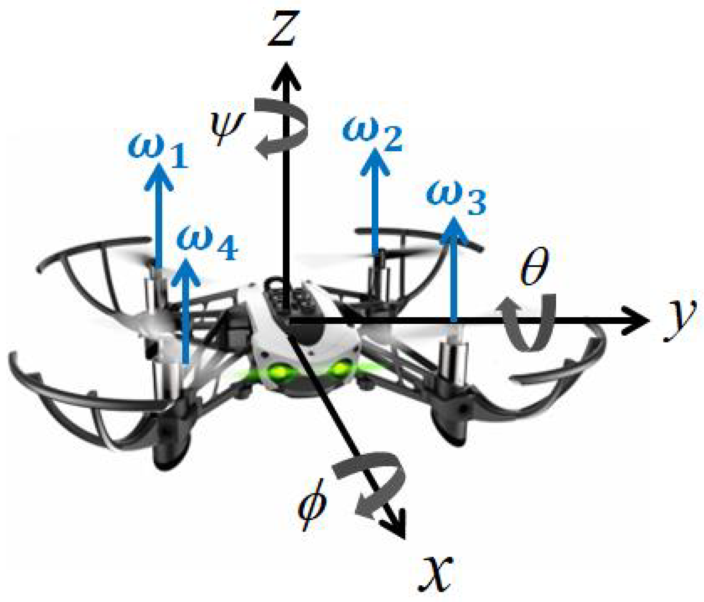
In this study, we used the Parrot Mambo quadrotor model as a reference. This model has four wing axes, making it suitable for applying the new model proposed in this study. Furthermore, because it has an appropriate size, it is suitable for conducting hardware experiments.
Figure 1 shows a structural diagram of the quadrotor used in the study.
As shown in
Figure 1, the quadrotor has three axes:
x,
y, and
z. The roll angle rotates around the
x-axis, the pitch angle rotates around the
y-axis, and yaw angle rotates around the
z-axis. For the quadrotor system used in this study, the roll and pitch attitude angles were limited to [−90 90], and the yaw angle was limited to [−180 180] to reflect practical quadrotor flight. Additionally, the differential values for the roll, pitch, and yaw angles can be expressed as
,
, and
. Based on these constraints, the state space can be defined as follows.
where
are the aerodynamic resistance,
m is the mass of the quadrotor,
g represents gravitational acceleration,
l is the distance from the center of the quadrotor to the actuators,
is the inertia coefficient of the actuator,
represent the control inputs,
represent the coefficients of inertia corresponding to each axis of the quadrotor,
is the overall angular speed of the actuators. Furthermore, when we define the state vector as
X = [
], the relationship between the control input and velocity of each actuator is as follows:
where
b and
a represent the thrust and drag coefficient, respectively.
Figure 2 shows the controller design. The flight inputs are generated based on the reference trajectory for the
x,
y, and
z coordinates and desired yaw angle. Therefore, this system can be classified as an underactuated system with four inputs and six degrees of freedom. Consequently, the desired values for the roll and pitch angles, besides the
x,
y,
z, and desired yaw values, must be derived based on the reference trajectory. As shown in Equation (
3), the control inputs
,
, and
correspond to the different axes and are necessary for achieving the hovering force in a quadrotor, which is an underactuated system. The lifting force
is defined as the sum of these control inputs, where the control input
is specifically used to derive the required hovering force
. In contrast, the control inputs
and
serve as auxiliary inputs to obtain the desired roll and pitch angles, respectively. Using these expressions, we can represent the control inputs
,
, and
as follows:
As mentioned previously, the quadrotor in this study was an underactuated system. Using the control input expression in Equation (
3), the desired roll and pitch angles must be generated to achieve six degrees of freedom. The desired roll and pitch angles are represented by the following equations:
A quadrotor model with six degrees of freedom can be established by generating the desired roll and pitch angles along with the desired
x,
y,
z, and yaw.
,
, and
are the desired roll, pitch, and yaw angles, respectively, with
given by the external order. This study was conducted using the quadrotor model represented in Equation (
4).
3. Design of Sliding Surface and Control Law
One of the key focuses of this study is the process of deriving control laws using the proposed method. The newly designed control inputs were then converted into motor commands for the Parrot Mambo quadrotor. The state of the quadrotor was measured using sensors. The error values for SMC are defined as follows,
In general, to define a sliding surface, the derivative of the error value also must be defined. On the sliding surface, the error value was multiplied by the sliding slope, and the derivative of the error value was added. To apply sliding mode control, sliding surfaces corresponding to the six degrees of freedom of the quadrotor must be defined. To simplify this representation, we considered Equation (
5) as the state vector and expressed the sliding surfaces as vectors. The sliding surfaces can be defined as follows:
Expressed in the matrix form, Equation (
6) can be rewritten as follows:
Here,
represent the sliding surfaces corresponding to the
x,
y,
z, roll, pitch, and yaw angles, respectively.
represent the sliding slopes associated with the six sliding surfaces. According to the principle of SMC, we can design six corresponding control laws as follows:
where
with
,
and
being the design parameters. Equation (
8) can be expressed as the sum of the equivalent controller and the reaching law. This signifies
in which the first part in front of the
term in all six equations represents the
, and the remaining terms denote the
proposed in this study. With Equation (
8), we can define the reaching law and demonstrate stability in the following section.
4. Stability Analysis
To prove the system stability of SOSMC, an approach different from the Lyapunov stability used in conventional SMC is required. Thus, SOSMC employs strict Lyapunov stability by utilizing two vector spaces to demonstrate system stability [
22]. Although the process of constructing the Lyapunov function differs, the procedure for creating the sliding surface remains unchanged. Hence, using Equation (
7) to generate the general sliding surface, the surface equation can be expressed as follows:
Here, we present the control law of the ASOSMC system proposed in this study. We derived an equation that allows for more stable flight without being affected by chattering through the additional robust control term to the reaching law of the conventional SOSMC, which is not influenced by the signum function. The proposed control law is as follows [
24,
25]:
where
s denotes the general sliding surface;
,
, and
are positive gains; and
. The reduction of
in the Equation (
11) implies that the
and
terms converge to
and 0, respectively. By supplementing a small gain to
, the system control performance can be satisfied and the part obtained from the
integration term can be eliminated. Meanwhile, increasing
means that
and
converge to
and
, subsequently becoming greater than
and
, respectively. This implies that it can produce a higher convergence rate than SOSMC system. Furthermore, because
and
are continuous parameters, the gains mitigate stress that occurs when the state changes rapidly. The proposed ASOSMC has an additional control gain compared to SOSMC, which results in a faster response speed. The control gain is bounded to a finite real number, which ensures broad stable region. Additionally, the use of an exponential function, which is a continuous function, resulted in chattering reduction effect.
In general, to prove the system stability of SOSMC, we must use a strict Lyapunov function. However, the proposed reaching law has three dimensions instead of the usual two dimensions used in SOSMC. Therefore, Equation (
11) is reorganized to reduce the dimensions to two and construct a Lyapunov function. Equation (
11) can be rewritten as follows:
We now apply a strict Lyapunov function, which can be expressed as follows:
where
Differentiating
with respect to time leads to the following expression:
P is a constant, symmetric, and positive definite matrix that represents a strict Lyapunov function without perturbation terms. The
P value satisfying these conditions can be set as follows:
Therefore, the Lyapunov function
V is positive definite. To prove the stability of the system, showing that the derivative of the Lyapunov function
V is negative is sufficient. Taking the derivative of
V yields the following expression:
Q can be expressed using the algebraic Lyapunov equation (ALE) [
22],
Therefore, rearranging Equation (
17),
can be expressed as follows:
Because
Q is positive,
is negative, indicating that the system is stable. Moreover, demonstrating that the system is stable within finite time is necessary. To achieve this, Equation (
11) must first be finite-time-stable for the initial state
. Additionally, the matrix
A should be Hurwitz, where all eigenvalues have negative real parts, and the constant gain should be positive (
,
). Under these conditions, the ALE satisfies
for every symmetric, positive matrix
Q. By differentiating
V,
is satisfied, and the value of
at
is smaller than that of
.
The following steps are performed to prove Equation (
20). As Equation (
16) is positive and radially unbounded, we can construct the following equation [
26,
27]:
With Equation (
13), we can rewrite Equation (
21) as follows:
In the first case, to prove the first condition of Equation (
22), we obtain the following result.
Since
, we can structure the first case as follows:
By multiplying the left side of Equation (
24) with
and substituting
P with
Q, we obtain the following equation.
In the second case, to prove the second condition of Equation (
22), the following result is obtained:
By moving
to the left side and multiplying both sides of Equation (
26) by
and using the same method as in Equation (
25), the following equation can be obtained.
Since
and
the following equation can be obtained.
Combining the first and second cases, we can obtain the following inequality.
The solution of the differential inequality represented as
is given by
Therefore, at least for
, the solution of
becomes
. Therefore,
converges to zero in finite time and reaches that value after a period given by Equation (
19) [
26,
27]. Thus, the system is finite-time-stable.
5. Silmulation
Evaluating the performance of the proposed reaching law and analyzing the flight characteristics via simulations are crucial. Therefore, we set up a simulation environment following these guidelines and conducted simulations based on the Parrot Mambo quadrotor model, which is a real quadrotor model. Instead of using the existing controller for the Parrot Mambo quadrotor model, we applied the newly developed ASOSMC method to examine its capability for a stable flight. In the simulation, we compared the performance of the ASOSMC with those of CSMC and SOSMC to evaluate the precision of the control achieved via the ASOSMC.
During the simulation, experiments were conducted using MATLAB Simulink. This enabled us to assess the performance of the proposed ASOSMC method compared to that of other methods. First, we set the parameter values based on Equation (
1), and the solver of the simulation was chosen as ODE3. The fixed sample period was set as 0.005 s.
Table 1 presents an overview of the parameters used in the simulations.
Table 1 lists the parameters used in Equation (
1). In addition to these parameters, the gain values for the proposed ASOSMC method, as well as for the comparison methods (CSMC and SOSMC), need to be provided. To perform a proper comparison of methods, not only the ASOSMC reaching law specified in Equation (
11) but also the reaching law for conventional SMC and SOSMC needs to be provided.
Table 2 presents the gain values for each method, along with information regarding the sliding slope. The reaching laws for conventional SMC and SOSMC are as follows:
Equations (
8) and (
9) represent the reaching law for conventional SMC and SOSMC, respectively. Here,
denotes the CSMC control gain, while
and
represent the control gains for SOSMC.
Table 2 presents the gain values for each method, along with information regarding the sliding slope. The gain values for ASOSMC are denoted as
to
. Additionally, the epsilon gain represents the gain value for parameter
in Equation (
9). In actual quadrotor flight, there exists potential discrepancies. Therefore, to address the similarity between simulation and hardware, a specific disturbance was introduced to mitigate potential discrepancies. The disturbances for the simulation experiments are considered as follows:
The simulations are constructed based on
Table 1 and
Table 2, and the fundamental trajectory is created by desired
,
,
, and yaw values. Here,
is a sine wave with an amplitude of 2 m,
is a cosine wave with an amplitude of 2 m,
is a step function with a magnitude of 1.5 m, and yaw is a desired trajectory with a value of 0 degrees. Additionally, according to Equation (
4), desired roll and pitch angles are generated. The experiments involved a 60 s quadrotor flight, during which an external disturbance was introduced at the 30 s mark. During the performance evaluation for three different methods, we conducted tests to assess the robustness to disturbances by applying step functions corresponding to the same value on the
x-axis and
y-axis, respectively. The goal was to evaluate and compare the control performance of the three methods and determine the method that demonstrated the best control performance.
Figure 3 depicts the quadrotor flight in 3D. A significant movement is observed along the
z-axis. To understand the cause of this movement, the block diagram shown in
Figure 2 must be analyzed. In
Figure 2, the
z and yaw controllers are separated from the
x and,
y controllers and roll and pitch controllers, respectively. If the
z controller does not initially provide sufficient force, instability can be introduced in the yaw angle, making control more difficult. Therefore, providing a larger initial hovering force facilitates smoother control of the system. This is attributed to the significant movement along the
z-axis in
Figure 4. Furthermore, the response of ASOSMC, SOSMC, and CSMC during the occurrence of a disturbances at the 30 s mark can be observed. Here, the ASOSMC demonstrates the most effective performance among the three methods.
Figure 4 illustrates the performance of quadrotor flight in terms of its six degrees of freedom when an external disturbance occurs.
Figure 4a–f show the variations in
x,
y,
z, roll, pitch, and yaw, respectively. Overall, the ASOSMC outperforms the other two methods. To examine flight stability further, the error values must be analyzed. As indicated by Equation (
10), the error values correspond to
, which enables a more detailed observation of their changes.
Generally, when the error approaches zero, the system is considered stable.
Figure 5 shows the error values of the quadrotor angles. The error values for position are omitted because in this quadrotor model, the angles are more significant than the position. Therefore, the error values of the angles were examined. Similarly to
Figure 4,
Figure 5 demonstrates that the proposed ASOSMC outperforms the other methods in terms of error performance.
The weakness of CSMC is the chattering phenomenon caused by the sign term. This chattering can impose stress on hardware and potentially disrupt flight operations. In contrast, the ASOSMC, which is based on SOSMC, demonstrates superior performance compared to other methods not only in stable flight but also in addressing the chattering issue.
Figure 6 illustrates the control input for attitude. As shown in
Figure 6, CSMC exhibits significant chattering, whereas SOSMC and ASOSMC effectively reduce the chattering phenomenon. Thus, the ASOSMC enables a more stable flight than does conventional SMC.


