Random Walks-Based Node Centralities to Attack Complex Networks

Abstract

Investigating the network response to node removal and the efficacy of the node removal strategies is fundamental to network science. Different research studies have proposed many node centralities based on the network structure for ranking nodes to remove. The random walk (RW) on networks describes a stochastic process in which a walker travels among nodes. RW can be a model of transport, diffusion, and search on networks and is an essential tool for studying the importance of network nodes. In this manuscript, we propose four new measures of node centrality based on RW. Then, we compare the efficacy of the new RW node centralities for network dismantling with effective node removal strategies from the literature, namely betweenness, closeness, degree, and k-shell node removal, for synthetic and real-world networks. We evaluate the dismantling of the network by using the size of the largest connected component (LCC). We find that the degree nodes attack is the best strategy overall, and the new node removal strategies based on RW show the highest efficacy in regard to peculiar network topology. Specifically, RW strategy based on covering time emerges as the most effective strategy for a synthetic lattice network and a real-world road network. Our results may help researchers select the best node attack strategies in a specific network class and build more robust network structures.

1. Introduction

Numerous studies have been conducted in recent years to explore the response of real-world networks to the removal of nodes [1,2,3,4,5,6,7]. These investigations simulate the consequences of node removal (attack) on the network and have applications in diverse scientific fields, such as ecology [5], transportation [8], informatics [9], neural [10,11], and social networks [12,13].

The main objectives of these studies are twofold. Firstly, they aim to assess networks’ robustness by measuring the system’s ability to maintain functionality after link and node removal. Secondly, they seek to identify the link and node removals that cause the most significant damage to the network, thereby uncovering the key players that significantly influence network functioning.

Analyzing attack strategies provides valuable insights into enhancing network resilience by anticipating threats and identifying elements requiring protection [5,6].

An attack strategy refers to the identification and implementation of methods or techniques that aim to disrupt or dismantle a network [5,6,7]. It also plays a crucial role in situations where network disruption is necessary, such as halting the spread of a disease or a computer virus or impeding the growth of a cancer cell [14,15,16].

Many centralities’ measurements have been proposed to select important nodes to remove. See [17] for a summary. Methods to measure node centralities are generally based on the topological structure of the network, such as removing nodes while accounting for their degree and betweenness [5,17,18]. The betweenness node removal strategy, which removes nodes according to their recalculated betweenness centrality, yields the best attack in 70–80% of the cases [17].

Other methods analyze dynamic processes on networks and then identify important nodes for these processes.

The graph burning problem (GBP) is introduced in the context of social contagion, and it may also model the spread of viral infections under a very idealistic context [19,20]. GBP furnishes the burning number, which quantifies how vulnerable to “contagion” a network is. In addition, the solution of GBP ranks node importance and consists of a set of critical nodes to attack to halt the epidemic spreading.

The firefighter problem (FFP) defines a discrete-time model of a diffusive process (e.g., a fire, a flood, an infectious disease, information, a computer virus, or an invasive species) where the fire originates from a set of network nodes [21,22]. A solution to the FFP furnishes the defending actions that have to be taken to optimally contain the spreading process by minimizing the number of burnt nodes to stop the diffusive process [22].

The random walk (RW) on networks describes a stochastic process in which a walker travels among nodes along network links [23,24]. RW can be a model of transport, diffusion, and search on networks [25,26]; it is a handy tool for studying the structure of networks [23] and the importance of network nodes [27,28,29].

This manuscript joins network attack simulation and random walk processes on networks. Here, we propose four new measures of node centrality based on RW. The new removal strategies focus on important notions in RW walks theory, such as the covering time, start node, and stop node. Then, we test the proposed node centralities as effective strategies to rank nodes to remove to dismantle the network on synthetic and real-world networks. We compare the efficacy of the new node removal strategies based on random walks with effective node removal strategies from the literature, namely betweenness, closeness, degree, and k-shell node removal.

2. Methods

2.1. Basic Notions

In this work, we consider binary and undirected networks $G\left(V,E\right)$, where $V$ and $E$ are the sets of nodes (vertices) and links (edges). $N=\left|V\right|$ indicates the number of nodes, and $L=\left|E\right|$ indicates the number of edges. We assume $G$ to be undirected. The symbol $A$ denotes the $N\times N$ adjacency matrix of $G$, having entries $a_{ij}$, for $i,j=1,\dots ,N$, such that $a_{ij}=1$ if $\left(i,j\right)\in E$, and $a_{ij}=0$ otherwise. A path between two nodes, $u$ and $w$, is a sequence of nodes $⟨v_1,\dots ,v_k⟩$ with $v_1=u$ and $v_k=w$, such that $\left(v_i,v_{i+1}\right)\in E$ for $i=1,\dots ,k-1$. The length of the path equals the number of edges it contains. The distance, $d_{ij}$, is the shortest path length between node $i$ and $j$. In this work, all considered networks are connected, i.e., a path exists between each pair of nodes in $V$.

The problem of finding if one graph is a subgraph of another graph is called Subgraph Isomorphism [30].

Given a pair of graphs, $H(V_H,E_H)$ and $G(V_G,E_G)$, the problem of checking if $H$ is a subgraph of $G$ consists in finding a bijection, $f:V_H\to V_G$, such that ($\left(u,v\right)$)$\in E_H$ if and only if ($\left(f\left(u\right),f\left(v\right)\right)$)$\in E_G$.

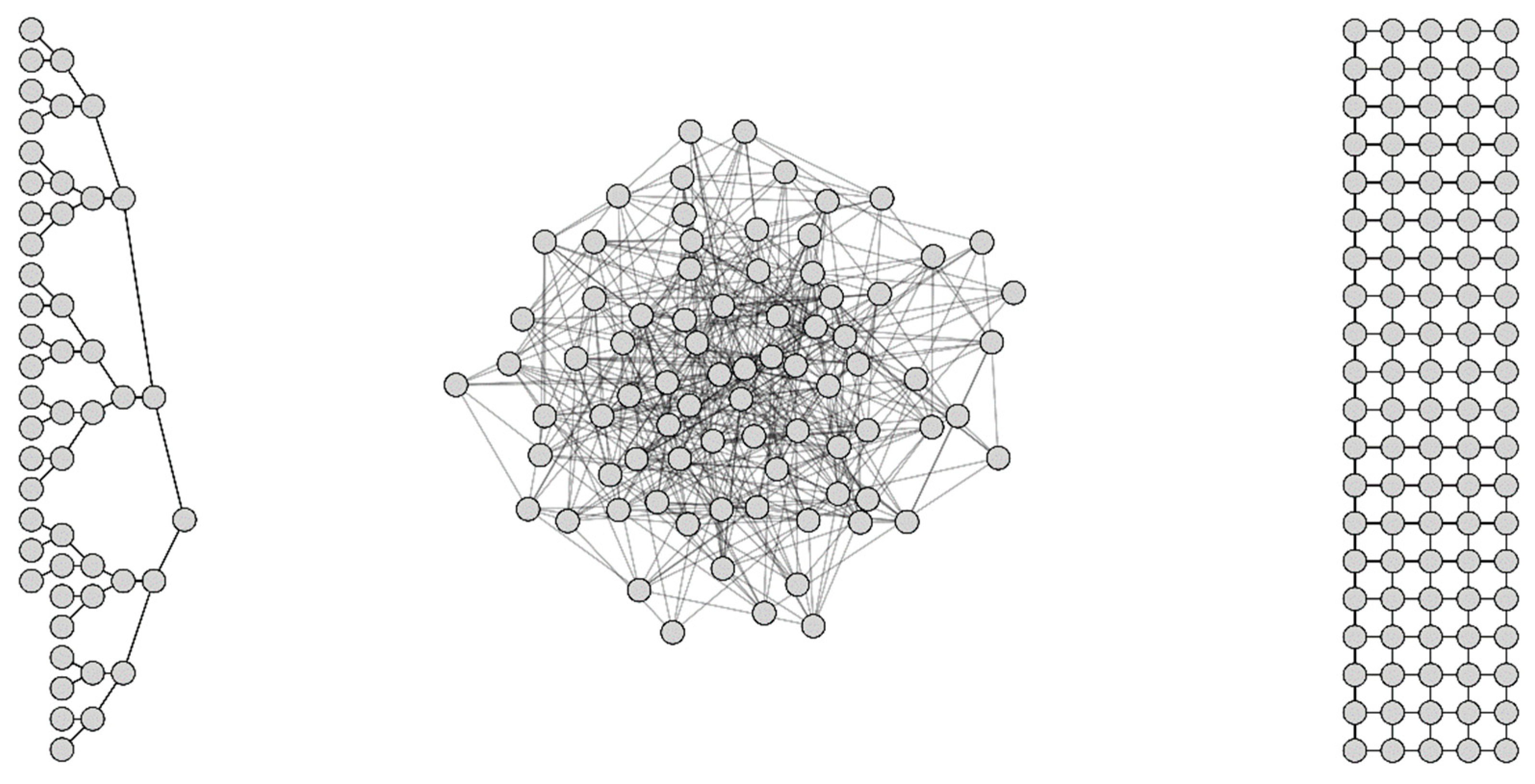
2.2. Synthetic Networks

• ER: classical Erdös–Rényi (ER) random graph [31]. In the ER model, each edge has a fixed probability of being present or absent, independent of the other edges. The ER graph is defined by two parameters only: the number of nodes, $N$; and the probability of drawn links, $p$. We indicate the $ER\left(N,p\right)$ of the $N$ (number of nodes) and $p$ (probability of links) between each pair of vertices. We investigate ER network with $N=80$ and $p=0.15$.
• LTC: rectangular (or square) lattice (LTC) complex network. A lattice graph is called a mesh or grid graph in graph theory. The LTC is a specific lattice graph where nodes form a grid with square meshes. The LTC can be defined by two parameters, $x$ and $y$, indicating the number of nodes along each side. We simulate two $LTC\left(x,y\right)$ networks by choosing $x=20$ and $y\in 5,20$ [32].
• BBT: balanced binary tree [33,34,35]. A balanced binary tree is a tree data structure in which the difference in height between the left and right subtrees of any node is, at most, one. A reduced version (for space constraints) with $50$ nodes is shown in Figure 1.

For the statistical relevance of the results obtained with $ER$ random graphs, we performed ${10}^3$ graph generations.

Figure 1 depicts examples of the synthetic networks used in this research.

2.3. Real-World Complex Networks

• Air Control: This network was constructed from the USA’s FAA (Federal Aviation Administration) National Flight Data Center (NFDC), Preferred Routes Database (Preferred Routes Database: http://www.fly.faa.gov/ accessed on 29 October 2023). The nodes in this network represent airports or service centers, and the links are created from strings of preferred routes recommended by the NFDC [36].
• Arenas Email: email communications among people working within a medium-sized university (i.e., Universitat Rovira i Virgily, Spain) with about $1700$ employees [25]. The nodes are employees, and the links describe the emailing among them.
• Barcelona Flow: models the traffic flow in Barcelona (Spain). The nodes represent intersections among roads, and the links represent roads [36].
• UK Faculty: personal friendship network within a faculty at a university in the UK. This network comprises 81 vertices representing individuals and edges representing their friendship relations [37].
• Netscience: a co-authorship network focusing on scientists involved in network science. The network represents collaborations among these scientists [29]. The nodes are scientists, and the links depict the co-authorship in scientific papers.
• Beijing 2^nd: represents the second ring road of Beijing City, China’s capital. The nodes and links represent road intersections and roads, respectively [38].
• Beijing 3^rd: represents the third ring road of Beijing City, China’s capital. The nodes and links represent road intersections and roads, respectively [38].
• Beijing 4^th: represents the fourth ring road of Beijing City, China’s capital. The nodes and links represent road intersections and roads, respectively [38].
• Beijing 5^th: represents the fifth ring road of Beijing City, China’s capital. The nodes and links represent road intersections and roads, respectively [38].
• Euroroad: a topological representation of international European roads in which the nodes represent intersections among roads, and the links represent roads [39].
• Little Rock Food Web: a model of trophic interactions among species of the Little Rock Lake ecosystem in Wisconsin. In this ecological network, the nodes represent living species, and the links represent the transfer of nutrients between them [40].
• Olocene Food Web: The Olocene Food Web ecological network is the basis of the 48 million years-old uppermost early Eocene Messel Shale food web. The nodes are biological species, and the links represent trophic relationships among them [41].
• San Francisco Reduced: represents a reduced version of the San Francisco road network [36] (Real Datasets for Spatial Databases, https://users.cs.utah.edu/~lifeifei/SpatialDataset.htm accessed on 29 October 2023) that was obtained by applying a simple spatial-partitioning algorithm, resulting in a smaller, computationally affordable graph for the scope of this work.
• Road Minnesota: the road map of Minnesota (US) [42]. The nodes represent intersections among roads, and the links represent roads.
• San Joaquin County: California (US) city road map [36] (Real Datasets for Spatial Databases, https://users.cs.utah.edu/~lifeifei/SpatialDataset.htm accessed on 29 October 2023). The nodes are the intersections among roads, and the links represent roads.

2.4. Network Structural Indicators

In

Table 1. Network structural indicator values for the synthetic and real-world networks analyzed.

Network	$\left|\mathit{V}\right|$	$\left|\mathit{E}\right|$	$\mathit{D}\mathit{i}\mathit{a}\mathit{m}$	$\overline{\mathit{k}}$	$\overline{\mathit{\delta }}$	$\mathit{C}\mathit{C}$	$\mathit{\rho }$
Air Control	1226	2410	17	3.931	5.924	0.064	0.003
Arenas Email	1133	5451	8	9.622	3.603	0.166	0.009
Barcelona Flow	930	1798	27	3.867	12.721	0.084	0.004
Beijing 2nd	144	233	19	3.236	7.813	0.011	0.023
Beijing 3rd	322	544	27	3.379	11.030	0.018	0.011
Beijing 4th	547	926	33	3.386	13.904	0.019	0.006
Beijing 5th	815	1308	48	3.210	17.246	0.024	0.004
Euroroad	1039	1305	62	2.512	18.377	0.035	0.002
Little Rock Food Web	183	2452	4	26.798	2.135	0.332	0.147
Netscience	379	914	17	4.823	6.026	0.431	0.013
Olocene Food Web	700	6425	6	18.357	2.629	0.074	0.026
Road Minnesota	2641	3303	100	2.501	35.349	0.028	0.001
San Francisco Reduced	435	440	41	2.023	17.461	0.000	0.005
San Joaquin County	7087	9793	50	2.764	13.939	0.000	0.000
UK Faculty	81	577	4	14.247	2.072	0.473	0.178
LTC (20,5)	100	175	23	3.500	8.250	0.000	0.035
LTC (20,20)	400	760	38	3.800	13.300	0.000	0.010
BBT	100	99	12	1.980	7.654	0.000	0.020
ER (N = 80, p = 0.15)	80.0	474.52	3.1	11.863	1.969	0.148	0.150

, we report network structural indicators that are useful for comparing the structure of the networks considered in this work. The network diameter, $Diam$, is the maximum length among all shortest paths between each pair of nodes [12]; the average node degree is the average number of links to the node, $\overline{k}$ [43]; the average clustering coefficient, $CC$, is the number of closed triplets (or triangles) over the total number of triplets (both open and closed) [44,45]; the average node distance, $\overline{\delta }$, is the average length of the shortest path among node pairs [12]; and the network density (or connectance), $\rho$, is the fraction of realized edges among all possible edges that can be drawn in the network [46,47].

2.5. Node Removal Strategies

Node removal (NR), also called node attack [48,49], refers to the process of selectively removing nodes from a network to study the impact on the structural properties of the network [13]. The removal strategy refers to how nodes are chosen to be removed from the network by assigning a value to each node and then defining an order in which to perform the NR.

In this paper, we define a series of RW-based node NR strategies and investigate their effectiveness in dismantling the networks. We compare their efficacy against four well-known centrality measures from the literature: closeness, betweenness, degree, and k-shell node removals. We quantify the network dismantling after NR by using the largest connected component (LCC)’s size. The node centrality rank is computed at the beginning of the simulation, i.e., before the first node removal. The NR is performed by following the order of node centrality and computing the LCC after each removal. In the case of ties, i.e., nodes with equal centrality values, we randomly sort the nodes. The node centralities and the simulation analyses are performed using the complex network analysis (CNA) library Graph Tool (Tiago P. Peixoto) [50], which consists of Python bindings for C++ and is highly performant, as it is based on the Boost Graph Library [51].

In the following, we define the NR strategies used in this work.

2.6. Betweenness Centrality

The betweenness centrality of a node $v\in V$, is defined as follows:

$$btw\left(v\right)=\sum _{s\ne v\ne t}\frac{{\sigma }_{st}\left(v\right)}{{\sigma }_{st}}$$

where ${\sigma }_{st}$ is the total number of shortest paths from $s$ to $t$, and ${\sigma }_{st}\left(v\right)$ is the number of shortest paths from $s$ to $t$ that pass through node $v$ [52].

2.7. Closeness Centrality

The closeness centrality of a node $v\in V$ is defined as follows:

$$cls\left(v\right)=\frac{1}{\sum _{u\ne v}{d}_{uv}}$$

where $d_{uv}$ represents the distance between node $u$ and node $v$ [53].

2.8. Degree Centrality

The degree centrality of a node $v\in V$ is defined as follows:

$$deg\left(v\right)=k$$

where $k$ is the number of links of $v$.

2.9. K-Shell Centrality

The k-shell [54] of graph $G(V,E)$ is closely related to the concept of k-core [55]. The k-core of $G$ is the largest subset of $V$ in which nodes induce a subgraph [30] where all nodes have degrees larger than or equal to $k$.

Consequently, the k-shell of a node $v\in V$ is defined as follows:

$$ksh\left(v\right)=k$$

where the $v$ $\in$ k-core of $G$ and $v\notin$ (K+1)-core of G.

2.10. Random Walk-Based Strategies

A simple random walk (RW) on $G$ is a graph traversal in which an agent moves from node $u$ to node $v$, such that $v$ is chosen with uniform probability among the (first) neighbors of $u$ [56]. Formally, the probability of transition from $u$ to $v$ can be defined as follows [57]:

$$p_{uv}=\frac{a_{uv}}{\sum _{w\in \tau }{a}_{uw}}$$

where $\tau$ is the neighbor’s node set of $u$, and $a_{uv}$ is the element of the adjacency matrix of $G$. The walk ends when all vertices have been visited at least once. The covering process refers to the process of visiting all the network nodes. We call the vertex from which the walk starts the “start node”. For statistical relevance of analysis, we averaged the results from ${10}^3$ RWs for each start node, $v\in V$. In the following part of this section, we define four RW-based strategies to perform node removals.

2.11. Recurrence Number

The recurrence number (RN) of a node is the number of times a random walker passes through the node during the covering process. Since the random walker covers all graph nodes, the simulation stops with a vector of RNs, one for each node. We call this vector of length, $\left|V\right|$, the recurrence vector (RV), and each RN is $>0$. In this node attack strategy, we remove nodes in decreasing order of the RN.

2.12. Stop Node

The stop node (SN) is the last node encountered by an RW, or, in other terms, the node where the RW stops its travel. The stop vector (SV) is the vector of length, $\left|V\right|$, in which the entry $i$ accounts for how many times the node $i$ acted as an SN. Since we iterate ${10}^3$ RW simulations, the sum of the SV entries is ${10}^3$. In this node attack strategy, we remove nodes in ascending order of the SN.

2.13. Cover Time

Given a vertex, $v\in V$, we call the time step the action of passing from $v$ to a (randomly chosen) neighbor. The cover time refers to the number of time steps needed to visit all graph nodes [58]. The cover time vector (CTV) is the vector of length, $\left|V\right|$, in which entry $i$ accounts for the CT when $i$ is the starting node. The CTV accounts for each source node, the corresponding CT. In this node attack strategy, we remove nodes in decreasing order of the CT: starting nodes producing a higher CT are removed first.

2.14. Stop Distance

Given a random walk on $G$, the stop distance (SD) is the distance, $d_{st}$, for $s,t\in V$, where $s$ and $t$ are, respectively, the start and the stop node of the random walk. The stop distance vector (SDV) is the vector of length, $\left|V\right|$, in which the entry $i$ accounts for the SD when $i$ is the starting node. The SDV stores the corresponding SD for each source node. In this node attack strategy, we remove nodes in ascending order of the SD: starting nodes near the stop node are removed first.

See Algorithm 1 for an explanation of the RW simulation analysis.

Algorithm 1: Methodology of the RW analysis.

$\mathbf{R}\mathbf{W}\left(\mathrm{G}\right(\mathrm{V},\mathrm{E}),\mathrm{s}\mathrm{t}\mathrm{a}\mathrm{r}\mathrm{t}\_\mathrm{n}\mathrm{o}\mathrm{d}\mathrm{e})$:

$\mathrm{r}\mathrm{e}\mathrm{c}\_\mathrm{n}\mathrm{u}\mathrm{m}\mathrm{b}\mathrm{e}\mathrm{r}\left[\mathrm{v}\right]\leftarrow 0,\forall \mathrm{v}∊\mathrm{V}$

rec_number[start_node] $\leftarrow$ 1

cov_time $\leftarrow$ 1

$\mathrm{s}\mathrm{t}\mathrm{o}\mathrm{p}\_\mathrm{n}\mathrm{o}\mathrm{d}\mathrm{e}\leftarrow \mathrm{s}\mathrm{t}\mathrm{a}\mathrm{r}\mathrm{t}\_\mathrm{n}\mathrm{o}\mathrm{d}\mathrm{e}$

$\mathrm{v}\leftarrow \mathrm{s}\mathrm{t}\mathrm{a}\mathrm{r}\mathrm{t}\_\mathrm{n}\mathrm{o}\mathrm{d}\mathrm{e}$

while ∃ x ∊ V | rec_num[x] == 0 do

u $\leftarrow$ randomly chose a neighbor of v

rec_num[u] $\leftarrow$ rec_num[u] + 1

stop_node $\leftarrow$ u

cov_time $\leftarrow$ cov_time + 1

v $\leftarrow$ u

end while

stop_distance $\leftarrow$ d(start_node, stop_node)

2.15. Network Robustness Indicator

2.15.1. Largest Connected Component

The largest connected component (LCC), also called the giant component [34], indicates the connected subgraph of $G$ having the largest set of nodes. In the literature, it has often been used as a network robustness indicator to evaluate the effectiveness of node or link removal strategies [14,59,60] by observing the decreasing trends of the LCC after such removals.

2.15.2. Robustness

The robustness value, $R$, represents the area under the curve of a decreasing trend of the LCC [17,59,61]. The lower the $R$, the higher the efficacy of the NR to dismantle the network. On the other hand, the higher the $R$, the lower the efficacy of the NR to dismantle the network. For clarity, we also define the inverse of robustness, $R^{-1}$. In this manner, higher $R^{-1}$ values denote more effective NR strategies.

Furthermore, given a fixed network, this value is normalized by the maximum value obtained among all NR strategies. This procedure allows us to compare the different robustness values obtained on a network while varying the different strategies. Additionally, given a fixed strategy, we denote $R_{avg}^{-1}$ as the average value of $R^{-1}$ obtained across all networks, allowing us to rank the average performance of each NR strategy across all networks.

Table 2. List of the abbreviations used in this manuscript.

LCC	(network’s) largest connected component
|V|	number of nodes in the network
|E|	number of links in the network
Diam	diameter of the network
$\overline{k}$	average node degree
$\overline{\mathsf{\delta }}$	average length of shortest path among all node pairs
CC	clustering coefficient, i.e., number of closed triples
ρ	network density, i.e., fraction of realized links in the network among all possible links
R	robustness of the network
$R^{-1}$	inverse of the network robustness
$R_{avg}^{-1}$	average inverse robustness, $R^{-1}$, among all networks
RN	recurrence number
CT	cover time
SN	stop node
SD	stop distance
BTW	betweenness centrality
CLS	closeness centrality
KSH	k-shell centrality
DEG	degree centrality

lists the abbreviations used in this manuscript.

3. Results and Discussion

In this study, we simulated random walk processes to cover the networks and evaluate node importance. We introduced four node attack strategies based on the simulated random walks process to assign each node a ranking (a value or score). Subsequently, we utilized these scores to define new node centrality measures. The introduced strategies include the recurrence number, stop node, stop distance, and covering time. Then, after attacking 19 networks—4 of which are synthetic and 15 of which are real-world networks—we compared the efficacy of dismantling the network of the new node centralities with four well-known competitors from the literature, namely betweenness (BTW), closeness (CLS), degree (DEG), and k-shell (KSH) node removals.

In Figure 2, we show the LCC decrease as a function of the node removal fraction for real-world networks, and in Figure 3, we show the same for the synthetic networks. Figure 4 displays the inverse of robustness, $R^{-1}$, normalized per row (i.e., per network), where each cell in the table is assigned a darker color as the strategy becomes more effective than the others. We report the average inverse robustness value across all networks in the last row.

Moreover, in Figure A1 and Figure A2 in Appendix A, we furnish the scatterplots of the random walk-based node centralities vs. the betweenness node centrality for the real-world networks, and in Figure A3 and Figure A4 in Appendix A, we depict the scatterplots of the random walk-based node centralities vs. the node degree centrality for the real-world networks.

In the following, we summarize and discuss the outcomes for each NR strategy.

BTW: Our results show that the well-known betweenness nodes attack (BTW) is an effective strategy overall, as it ranks second among the examined strategies, with an $R_{avg}^{-1}\approx 0.96$ (Figure 4). The BTW was the most effective on both food webs, UK Faculty, Arenas Email, and Beijing $5^{\mathrm{t}\mathrm{h}}$. It has also achieved good results on synthetic networks, particularly the ER networks and BBT. The performance of the BTW remains quite good because the $R^{-1}>0.7$ for all other networks but Euroroad. These results confirm previous studies indicating that betweenness is a very effective strategy for dismantling complex networks [5,17].

CLS: While the closeness nodes attack (CLS) performs poorly on most road maps, it is particularly effective on UK Faculty, Little Rock Food Web, and Arenas Email regarding real-world networks. Regarding synthetic networks, it exhibits a fairly good performance overall, especially on ER, BBT, and LTC$\left(20,20\right)$. The CLS ranks seventh among the examined strategies, with an $R_{avg}^{-1}\approx 0.68$.

DEG: This strategy is particularly effective on real-world road networks (Figure 4), where the removal of hubs according to their degree greatly impacts the dismantling process. The DEG ranks first among all tested strategies, with and $R_{avg}^{-1}=1$, resulting in the top strategy on eight networks and maintaining a high level of performance on all real-world networks, with an $R^{-1}>0.84$. Removing nodes based on their degree requires local information only; for this, the node degree attack is a strategy with a low computational cost. The low computational cost and the good performance confirm this strategy to be a good candidate for network dismantling.

KSH: The k-shell emerges as a generally effective strategy. Among real-world networks, it ranks first on Beijing 3^rd and performs well on San Joaquin County ($R^{-1}\approx 0.91$) and Beijing 4^th ($R^{-1}\approx 0.95$). Among synthetic networks, KSH proves effective on lattices, ranking first on LTC(20,20) and having an $R^{-1}\approx 0.95$ on LTC(20,5). KSH ranks fourth among all tested strategies, with an $R_{avg}^{-1}\approx 0.80$.

SN: The stop node (SN) has notable effectiveness on the ER random graph. Regarding real-world networks, the SN is the most effective on Barcelona Flow and the second most effective on UK Faculty. It also demonstrates good effectiveness on Beijing 2^nd and 4^th, as well as on Road Minnesota. The SN is the fifth strategy regarding average effectiveness, with an $R_{avg}^{-1}\approx 0.76$.

We defined the stop node as the node where the RW stops its travel. For this reason, nodes acting many times as stop nodes are likely to be peripheral nodes, with a very low probability of encountering an RW. On the contrary, nodes that never (or rarely) acted as a stop node are likely to be central in the network and encounter an RW. The SN strategy removes nodes in the ascending order of stop nodes, thus removing the central nodes first.

CT: The covering time (CT) proved effective on LTC$\left(20,20\right)$, and two real-world networks, Beijing 3^rd and 4^th. It also exhibited noteworthy effectiveness on Beijing 2^nd and ER. The CT ranks last in terms of average effectiveness, with an $R_{avg}^{-1}\approx 0.65$. The covering time is the number of time steps that the RW needs to pass over all nodes in the network [58]. The CT node attack strategy removes nodes in decreasing order of their covering time when they are the start node. This way, start nodes producing higher covering times are removed first. The CT strategy returns peculiar results: on the one hand, the CT showed the worst average efficacy (lowest $R_{avg}^{-1}$); on the other hand, it performed well in dismantling one synthetic and two real-world networks. The synthetic network is the square grid LTC, i.e., the model network with a planar structure and highly homogeneous node degree. In Figure 5, we depict the twenty most central nodes for each node removal strategy for the LTC networks of different sizes. The twenty most central nodes selected by the CT strategy are distributed over the entire network. In contrast, the most central nodes reside in a central part of the network for all the other strategies. Therefore, if we remove the highest BTW nodes from the LTC network, a large LCC composed of the peripheral nodes of the network will survive (see Figure 5). In other terms, the CT selects nodes covering the whole network structure, and for this, removing nodes according to the CT strategy may cause a faster LCC dismantling.

The two real-world networks where the CT is highly effective are the road networks of the Beijing ring. This road network shows a planar-like structure and a narrow range of node degrees (see Figure 6). Therefore, an interesting ability of the CT node attack strategies emerges to dismantle the networks with the specific characteristics of the planar-like structure and homogeneous node degree. In Figure 7, we depict the fifty most central nodes for each node removal strategy for the Road Minnesota and the Beijing 3^rd road networks. Like what was observed for the LTC, the fifty most central nodes, according to the CT strategy, are distributed over the entire network. In contrast, for all the other strategies, most central nodes reside in a part of the network. Therefore, this CT-specific node rank property may effectively dismantle real-world networks with a planar-like structure and homogeneous node degree, such as road networks.

SD: The stop distance (SD) performs well on synthetic graphs, particularly on LTC$\left(20,5\right)$, thus proving itself to be the most effective strategy. As for real networks, it demonstrates a solid performance on Olocene Food Web, UK Faculty, Arenas Email, and Beijing 2^nd. The SD is the sixth strategy regarding average effectiveness, with an $R_{avg}^{-1}\approx 0.69$. We defined the stop distance for a pair of nodes, $s$ and $t$, the shortest path length between the start node, $s$, and the stop node, $t$, of the random walk. The SD attack strategy removes nodes in ascending order of stop distance.

For this reason, the SD first removes the start nodes that are a small distance from the respective stop node. This strategy emerges as a particularly effective node removal over the lower dimension synthetic network square lattice LTC. As shown in Figure 5, the SD strategy can select nodes whose removals trigger the disruption of the LCC network in two parts. Therefore, removing nodes near their stop nodes can be a good method to dismantle this kind of model network and consequently select important nodes for its robustness.

RN: For a sufficiently large number of iterations, the recurrence number (RN) is proportional to the degree (see Figure A3 and Figure A4 in the Appendix A). As easily verified, the degree vector is the eigenvector of the transition matrix corresponding to the eigenvalue 1 (Perron–Frobenius eigenvector) [62]. Given this property, the RN is a degree-like node removal strategy and can be generally effective on most networks. Specifically, RN is the top strategy for the San Joaquin County road network. Additionally, it maintains an average level of effectiveness, $R^{-1}$, greater than 0.74 on all other real networks, seven of which have an $R^{-1}>0.9$. As for synthetic networks, it is less effective on lattices (LTC) where ${0.68<R}^{-1}<0.72$ and ineffective on BBT. RN is the third most effective strategy among the tested networks, with an $R_{avg}^{-1}\approx 0.92$.

4. Conclusions

Finding the best node attack strategy to dismantle the network is a paramount problem in network science [3,5,17,18]. In this manuscript, we proposed four new node removal strategies based on a simulated random walk on the network and compared them with well-known strategies from the literature. The well-known node removal strategies based on the node degree and betweenness resulted in the best strategies. Nonetheless, the random walk-based node removal proposed here presents a peculiar and high effectiveness on specific network structures. The CT strategy of removing nodes in decreasing order of the covering time they produce when they are the starting node is highly effective in dismantling planar-like and homogenous node degree network structures, such as road and square lattice networks. The methodology presented here can open future research. On the one hand, the node removal strategy proposed here can be helpful for another significant network science problem, such as finding the most influential spreader nodes in the network [63]. On the other hand, it will be interesting to investigate the efficacy of the random walk-based node attack strategies proposed here to lower other network robustness indicators, such as network efficiency [53].

A possible shortcoming of the proposed node removal strategies based on a simulated random walk can be the simulation cost. Nonetheless, we can say that dynamic processes based on random walks have become computationally more accessible than they were two decades ago. It is now possible to establish a series of statistically significant simulations by using tools such as the one used in Reference [50] that are adequately optimized for conducting small-scale simulations like the ones presented in this study. Our objective in further investigating these topics is to migrate our codes, making them suitable for harnessing parallel hardware in the HPC environment and enabling the simulation of such processes on large-scale graphs. Moreover, we aim to introduce new strategies that facilitate the exploration of the novel properties of real networks, which are often challenging to access solely through theoretical analysis.

References

1. Cohen, R.; Havlin, S. Complex Networks: Structure, Robustness and Function; Cambridge University Press: Cambridge, UK, 2010. [Google Scholar]
2. Cohen, R.; Erez, K.; Ben-Avraham, D.; Havlin, S. Resilience of the Internet to Random Breakdowns. Phys. Rev. Lett. 2000, 85, 4626. [Google Scholar] [CrossRef]
3. Morone, F.; Makse, H.A. Influence Maximization in Complex Networks through Optimal Percolation. Nature 2015, 524, 65–68. [Google Scholar] [CrossRef]
4. Callaway, D.S.; Newman, M.E.J.; Strogatz, S.H.; Watts, D.J. Network Robustness and Fragility: Percolation on Random Graphs. Phys. Rev. Lett. 2000, 85, 5468. [Google Scholar] [CrossRef]
5. Bellingeri, M.; Cassi, D.; Vincenzi, S. Efficiency of Attack Strategies on Complex Model and Real-World Networks. Phys. A Stat. Mech. Its Appl. 2014, 414, 174–180. [Google Scholar] [CrossRef]
6. Huang, X.; Gao, J.; Buldyrev, S.V.; Havlin, S.; Stanley, H.E. Robustness of Interdependent Networks under Targeted Attack. Phys. Rev. E 2011, 83, 65101. [Google Scholar] [CrossRef]
7. Nie, T.; Guo, Z.; Zhao, K.; Lu, Z.-M. New Attack Strategies for Complex Networks. Phys. A Stat. Mech. Its Appl. 2015, 424, 248–253. [Google Scholar] [CrossRef]
8. Pagani, A.; Mosquera, G.; Alturki, A.; Johnson, S.; Jarvis, S.; Wilson, A.; Guo, W.; Varga, L. Resilience or Robustness: Identifying Topological Vulnerabilities in Rail Networks. R. Soc. Open Sci. 2019, 6, 181301. [Google Scholar] [CrossRef]
9. Cohen, R.; Erez, K.; Ben-Avraham, D.; Havlin, S. Breakdown of the Internet under Intentional Attack. Phys. Rev. Lett. 2001, 86, 3682. [Google Scholar] [CrossRef]
10. Bassett, D.S.; Bullmore, E.D. Small-World Brain Networks. Neuroscientist 2006, 12, 512–523. [Google Scholar] [CrossRef]
11. Bullmore, E.; Sporns, O. Complex Brain Networks: Graph Theoretical Analysis of Structural and Functional Systems. Nat. Rev. Neurosci. 2009, 10, 186–198. [Google Scholar] [CrossRef]
12. Borgatti, S.P.; Mehra, A.; Brass, D.J.; Labianca, G. Network Analysis in the Social Sciences. Science 2009, 323, 892–895. [Google Scholar] [CrossRef]
13. Boldi, P.; Rosa, M.; Vigna, S. Robustness of Social and Web Graphs to Node Removal. Soc. Netw. Anal. Min. 2013, 3, 829–842. [Google Scholar] [CrossRef]
14. Sartori, F.; Turchetto, M.; Bellingeri, M.; Scotognella, F.; Alfieri, R.; Nguyen, N.-K.-K.; Le, T.-T.; Nguyen, Q.; Cassi, D. A Comparison of Node Vaccination Strategies to Halt SIR Epidemic Spreading in Real-World Complex Networks. Sci. Rep. 2022, 12, 21355. [Google Scholar] [CrossRef]
15. Nguyen, N.-K.-K.; Nguyen, T.-T.; Nguyen, T.-A.; Sartori, F.; Turchetto, M.; Scotognella, F.; Alfieri, R.; Cassi, D.; Nguyen, Q.; Bellingeri, M. Effective Node Vaccination and Containing Strategies to Halt SIR Epidemic Spreading in Real-World Face-to-Face Contact Networks. In Proceedings of the 2022 RIVF International Conference on Computing and Communication Technologies (RIVF), Ho Chi Minh City, Vietnam, 20–22 December 2022; pp. 1–6. [Google Scholar]
16. Bellingeri, M.; Turchetto, M.; Bevacqua, D.; Scotognella, F.; Alfieri, R.; Nguyen, Q.; Cassi, D. Modeling the Consequences of Social Distancing over Epidemics Spreading in Complex Social Networks: From Link Removal Analysis to SARS-CoV-2 Prevention. Front. Phys. 2021, 9, 681343. [Google Scholar] [CrossRef]
17. Wandelt, S.; Sun, X.; Feng, D.; Zanin, M.; Havlin, S. A Comparative Analysis of Approaches to Network-Dismantling. Sci. Rep. 2018, 8, 13513. [Google Scholar] [CrossRef]
18. Iyer, S.; Killingback, T.; Sundaram, B.; Wang, Z. Attack Robustness and Centrality of Complex Networks. PLoS ONE 2013, 8, e59613. [Google Scholar] [CrossRef]
19. Bessy, S.; Bonato, A.; Janssen, J.; Rautenbach, D.; Roshanbin, E. Burning a Graph Is Hard. Discret. Appl. Math. 2017, 232, 73–87. [Google Scholar] [CrossRef]
20. García-Díaz, J.; Rodríguez-Henríquez, L.M.X.; Pérez-Sansalvador, J.C.; Pomares-Hernández, S.E. Graph Burning: Mathematical Formulations and Optimal Solutions. Mathematics 2022, 10, 2777. [Google Scholar] [CrossRef]
21. Hartnell, B.; Rall, D.F. A Characterization of Graphs in Which Some Minimum Dominating Set Covers All the Edges. Czechoslov. Math. J. 1995, 45, 221–230. [Google Scholar] [CrossRef]
22. Gutiérrez-De-La-Paz, B.R.; García-Díaz, J.; Menchaca-Méndez, R.; Montenegro-Meza, M.A.; Menchaca-Méndez, R.; Gutiérrez-De-La-Paz, O.A. The Moving Firefighter Problem. Mathematics 2022, 11, 179. [Google Scholar] [CrossRef]
23. Burioni, R.; Cassi, D. Random Walks on Graphs: Ideas, Techniques and Results. J. Phys. A Math. Gen. 2005, 38, R45. [Google Scholar] [CrossRef]
24. Masuda, N.; Porter, M.A.; Lambiotte, R. Random Walks and Diffusion on Networks. Phys. Rep. 2017, 716–717, 1–58. [Google Scholar] [CrossRef]
25. Guimer, R.; Danon, L.; Diaz-Guilera, A.; Giralt, F.; Arenas, A. Self-Similar Community Structure in a Network of Human Interactions. Phys. Rev. E 2003, 68, 65103. [Google Scholar] [CrossRef] [PubMed]
26. Agliari, E. Exact Mean First-Passage Time on the T-Graph. Phys. Rev. E 2008, 77, 11128. [Google Scholar] [CrossRef] [PubMed]
27. Noh, J.D.; Rieger, H. Random Walks on Complex Networks. Phys. Rev. Lett. 2004, 92, 118701. [Google Scholar] [CrossRef]
28. Rocha, L.E.C.; Masuda, N. Random Walk Centrality for Temporal Networks. New J. Phys. 2014, 16, 63023. [Google Scholar] [CrossRef]
29. Newman, M.E.J. Analysis of Weighted Networks. Phys. Rev. E 2004, 70, 56131. [Google Scholar] [CrossRef] [PubMed]
30. Cordella, L.P.; Foggia, P.; Sansone, C.; Vento, M. A (Sub)Graph Isomorphism Algorithm for Matching Large Graphs. IEEE Trans. Pattern Anal. Mach. Intell. 2004, 26, 1367–1372. [Google Scholar] [CrossRef]
31. Erdös, P.; Rényi, A. On Random Graph I. Publ. Math. 1959, 6, 290–297. [Google Scholar] [CrossRef]
32. Acharya, B.D.; Gill, M.K. On the Index of Gracefulness of a Graph and the Gracefulness of Two-Dimensional Square Lattice Graphs. Indian J. Math. 1981, 23, 14. [Google Scholar]
33. Cormen, T.; Leiserson, C.; Rivest, R.; Stein, C. Introduction to Algorithms; MIT Press: Cambridge, MA, USA, 2009. [Google Scholar]
34. Van Steen, M. Graph Theory and Complex Networks: An Introduction; 2010; Volume 144. [Google Scholar]
35. Chen, G.; Wang, X.; Li, X. Fundamentals of Complex Networks: Models, Structures and Dynamics; John Wiley & Sons: Hoboken, NJ, USA, 2014; Volume 96. [Google Scholar]
36. Kunegis, J. Konect: The Koblenz Network Collection. In Proceedings of the 22nd International Conference on World Wide Web, Rio de Janeiro, Brazil, 13–17 May 2013; pp. 1343–1350. [Google Scholar]
37. Nepusz, T.; Petróczi, A.; Négyessy, L.; Bazsó, F. Fuzzy Communities and the Concept of Bridgeness in Complex Networks. Phys. Rev. E 2008, 77, 16107. [Google Scholar] [CrossRef]
38. Guo, X.-L.; Lu, Z.-M. Urban Road Network and Taxi Network Modeling Based on Complex Network Theory. J. Inf. Hiding Multim. Signal Process. 2016, 7, 558–568. [Google Scholar]
39. Šubelj, L.; Bajec, M. Robust Network Community Detection Using Balanced Propagation. Eur. Phys. J. B 2011, 81, 353–362. [Google Scholar] [CrossRef]
40. Martinez, N.D. Artifacts or Attributes? Effects of Resolution on the Little Rock Lake Food Web. Ecol. Monogr. 1991, 61, 367–392. [Google Scholar] [CrossRef]
41. Dunne, J.A.; Labandeira, C.C.; Williams, R.J. Highly Resolved Early Eocene Food Webs Show Development of Modern Trophic Structure after the End-Cretaceous Extinction. Proc. R. Soc. B Biol. Sci. 2014, 281, 20133280. [Google Scholar] [CrossRef]
42. Rossi, R.A.; Ahmed, N.K. The Network Data Repository with Interactive Graph Analytics and Visualization. In Proceedings of the Twenty-Ninth AAAI Conference on Artificial Intelligence, Austin, TX, USA, 25–30 January 2015. [Google Scholar]
43. Bellingeri, M.; Montepietra, D.; Cassi, D.; Scotognella, F. The Robustness of the Photosynthetic System I Energy Transfer Complex Network to Targeted Node Attack and Random Node Failure. J. Complex Netw. 2021, 10, cnab050. [Google Scholar] [CrossRef]
44. Boccaletti, S.; Latora, V.; Moreno, Y.; Chavez, M.; Hwang, D.-U. Complex Networks: Structure and Dynamics. Phys. Rep. 2006, 424, 175–308. [Google Scholar] [CrossRef]
45. Gleeson, J.P.; Melnik, S.; Hackett, A. How Clustering Affects the Bond Percolation Threshold in Complex Networks. Phys. Rev. E 2010, 81, 66114. [Google Scholar] [CrossRef]
46. Dunne, J.A.; Williams, R.J.; Martinez, N.D. Network Structure and Biodiversity Loss in Food Webs: Robustness Increases with Connectance. Ecol. Lett. 2002, 5, 558–567. [Google Scholar] [CrossRef]
47. Bellingeri, M.; Vincenzi, S. Robustness of Empirical Food Webs with Varying Consumer’s Sensitivities to Loss of Resources. J. Theor. Biol. 2013, 333, 18–26. [Google Scholar] [CrossRef]
48. Nguyen, Q.; Pham, H.-D.; Cassi, D.; Bellingeri, M. Conditional Attack Strategy for Real-World Complex Networks. Phys. A Stat. Mech. Its Appl. 2019, 530, 121561. [Google Scholar] [CrossRef]
49. Albert, R.; Barabási, A.-L. Statistical Mechanics of Complex Networks. Rev. Mod. Phys. 2002, 74, 47. [Google Scholar] [CrossRef]
50. Tiago, P. Peixoto Graph-Tool, Efficient Network Analysis. Available online: https://Graph-Tool.Skewed.De/ (accessed on 29 October 2023).
51. Siek, J.G.; Lee, L.-Q.; Lumsdaine, A. The Boost Graph Library: User Guide and Reference Manual; Addison-Wesley Professional: Boston, MA, USA, 2001. [Google Scholar]
52. Freeman, L.C. A Set of Measures of Centrality Based on Betweenness. Sociometry 1977, 40, 35–41. [Google Scholar] [CrossRef]
53. Marchiori, M.; Latora, V. Harmony in the Small-World. Phys. A Stat. Mech. Its Appl. 2000, 285, 539–546. [Google Scholar] [CrossRef]
54. Carmi, S.; Havlin, S.; Kirkpatrick, S.; Shavitt, Y.; Shir, E. A Model of Internet Topology Using K-Shell Decomposition. Proc. Natl. Acad. Sci. USA 2007, 104, 11150–11154. [Google Scholar] [CrossRef] [PubMed]
55. Batagelj, V.; Zaveršnik, M. Fast Algorithms for Determining (Generalized) Core Groups in Social Networks. Adv. Data Anal. Classif. 2011, 5, 129–145. [Google Scholar] [CrossRef]
56. Campari, R.; Cassi, D. Random Collisions on Branched Networks: How Simultaneous Diffusion Prevents Encounters in Inhomogeneous Structures. Phys. Rev. E 2012, 86, 21110. [Google Scholar] [CrossRef]
57. Xia, F.; Liu, J.; Nie, H.; Fu, Y.; Wan, L.; Kong, X. Random Walks: A Review of Algorithms and Applications. IEEE Trans. Emerg. Top. Comput. Intell. 2019, 4, 95–107. [Google Scholar] [CrossRef]
58. Lovász, L. Random Walks on Graphs. In Combinatorics, Paul Erdos Is Eighty; János Bolyai Mathematical Society: Budapest, Hungary, 1993; Volume 2, p. 4. [Google Scholar]
59. Bellingeri, M.; Bevacqua, D.; Scotognella, F.; Cassi, D. The Heterogeneity in Link Weights May Decrease the Robustness of Real-World Complex Weighted Networks. Sci. Rep. 2019, 9, 10692. [Google Scholar] [CrossRef]
60. Zhang, Y.; Ng, S.T. Identification and Quantification of Node Criticality through EWM–TOPSIS: A Study of Hong Kong’s MTR System. Urban Rail Transit 2021, 7, 226–239. [Google Scholar] [CrossRef]
61. Schneider, C.M.; Moreira, A.A.; Andrade, J.S., Jr.; Havlin, S.; Herrmann, H.J. Mitigation of Malicious Attacks on Networks. Proc. Natl. Acad. Sci. USA 2011, 108, 3838–3841. [Google Scholar] [CrossRef] [PubMed]
62. Levin, D.A.; Peres, Y. Markov Chains and Mixing Times; American Mathematical Society: Providence, RI, USA, 2017; Volume 107. [Google Scholar]
63. Kitsak, M.; Gallos, L.K.; Havlin, S.; Liljeros, F.; Muchnik, L.; Stanley, H.E.; Makse, H.A. Identification of Influential Spreaders in Complex Networks. Nat. Phys. 2010, 6, 888–893. [Google Scholar] [CrossRef]
Figure 1. The picture displays examples of the synthetic networks used in this study. From left to right, the reported networks are BBT (50 nodes), ER (n = 80; p = 0.15), and LTC (20, 5).
Mathematics 11 04827 g001
Figure 2. Impact of NR strategies on real-world networks: LCC (y-axis) as a function of the fraction of removed nodes (x-axis).
Mathematics 11 04827 g002
Figure 3. Impact of NR strategies on synthetic networks: LCC (y-axis) as a function of the fraction of removed nodes (x-axis).
Mathematics 11 04827 g003
Figure 4. Inverse network robustness, R 1 , for each network analyzed. To compare the efficacy of the node attack strategies, we normalize R 1 with its maximum value for each network. In this way, the maximum R 1 for each network equals 1. The higher the R 1 , the more effective the attack strategies to dismantle the network. In the last row, we depict the average R 1 value for all networks. The darker cell color indicates a higher R 1 .
Mathematics 11 04827 g004
Figure 5. Top row, the twenty most central nodes according to each node removal strategy for the LTC 20 , 5 . Bottom row, the twenty most central nodes according to each node removal strategy for the LTC 20 , 20 . The vertex size accounts for its centrality value: bigger nodes present a higher centrality value.
Mathematics 11 04827 g005
Figure 6. An illustrative example showcasing the structural approximation of a lattice by specific portions of a road map. The left network is the Beijing 3rd ring road network. The right network is the Road Minnesota network.
Mathematics 11 04827 g006
Figure 7. The fifty most central nodes according to each node removal strategy. The upper row network is the Road Minnesota network. The lower row network is the Beijing 3rd ring road network. The vertex size accounts for its centrality value: bigger nodes present a higher centrality value.
Mathematics 11 04827 g007