Modeling the Five-Element Windkessel Model with Simultaneous Utilization of Blood Viscoelastic Properties for FFR Achievement: A Proof-of-Concept Study

Abstract

Coronary artery diseases (CADs) are a leading cause of death worldwide. Accurate numerical simulations of coronary blood flow, especially in high-risk atherosclerotic patients, have been a major challenge for clinical applications. This study pioneers a novel approach combining the physiologically accurate five-element Windkessel and sPTT models to enhance the accuracy of the hemodynamics and the fractional flow reserve (FFR) parameter. User-defined functions (UDFs) of the outlet pressure boundary condition (Windkessel model) and the viscoelastic characteristics of blood (sPTT model) were developed and dynamically loaded with ANSYS^® 2023 software. In a proof-of-concept study, a patient’s left coronary artery with 40% stenosis was provided by the hospital for further analysis. The numerical FFR value obtained in the present work skews only 0.37% from the invasive measurement in the hospital. This highlights the important roles of both blood viscoelasticity and the five-element Windkessel model in hemodynamic simulations. This proof-of-concept of the FFR numerical calculation tool provides a promising comprehensive assessment of atherosclerosis in a fast, accurate, more affordable, and fully non-invasive manner. After validation with more patient cases in the future, this tool could be employed in hospitals and offer a more accurate and individualized approach for the diagnosis and treatment of CAD.

1. Introduction

Coronary artery disease (CAD) occurs when there is partial or total obstruction of the coronary arteries through the development of plaque in the lumen (stenosis), reducing the capacity of this organ (ischemia). This disease represents approximately one in three deaths in developed countries since it is potentiated by population aging and poor lifestyle choices [1]. Stenoses are assessed by medical doctors through the analysis of images obtained with computed tomography (CT) scans [2]. There is an objective parameter used to measure the impact that the stenosis has on the blood flow—the fractional flow reserve (FFR)—which is a measure of pressure drop that occurs in the lumen of the artery. This parameter is non-dimensional, with values between zero (the artery is completely blocked) and one (there are no obstructions to blood flow).

The current invasive method for calculating FFR involves introducing a wire into the stenosed artery while under hyperemic circumstances (maximum vasodilation induced by administration of adenosine), measuring two pressure values, namely the aortic pressure and then the pressure distal to the stenosis at exactly 20 mm downstream [3]. The FFR is defined as the ratio between distal and aortic pressures, p_d and p_a, respectively.

A stenosis is considered significant if the FFR is less than 0.75, and revascularization procedures are conducted to assure reasonable blood flow. Moreover, the narrowing is seen as having a mild impact if this parameter is greater than 0.8. For this case, the patient is provided with medication and a set of preventive measures is recommended, such as lifestyle changes. However, for intermediate values, the clinician is the one that determines which treatment would produce the best outcome, which may not always be the one chosen [4].

As alternatives to the invasive method, a growing body of research has focused on using computational fluid dynamics (CFD) in conjunction with CT images to create artificial models of the diseased arteries and solve numerical simulations of fluid dynamics for coronary blood flow and determine FFR values non-invasively [5,6,7,8,9]. Thus, the non-invasive process would be a viable and cost-free alternative, with no risk for the patient, aimed at improving the accuracy of the diagnostic process.

Windkessel models are lumped-parameter models used to represent the entire circulatory system and are based on the simplified representation of the different cardiovascular elements such as the heart and venous and arterial vessel structures [10]. Applying these models as boundary conditions allows for the creation of a pressure distribution profile along the entire vessel, eliminating the need to model the full circulatory system.

Jonášová et al. (2021) utilized several accurate Windkessel models with 3, 5, and 7 elements, to numerically assess coronary circulation, but they used the Newtonian and shear-thinning blood models, and did not evaluate the fractional flow reserve [11]. Kim et al. (2014) compared the invasive and the computed FFR measures of patient-specific left coronary arteries and found remarkably similar results. However, the study does not disclose the used boundary conditions, namely, which lumped-parameter model was used to model pressure, as well as the rheological model used to model the viscosity of blood. In addition, the numerical FFR results presented in the paper were calculated in the patient’s resting conditions [12]. Nakazato et al. (2013) performed a numerical study with 252 patients using blood as a Newtonian model and a lumped-parameter model. Though the model was able to overall match the invasive FFR, the simulation settings are not disclosed [13]. The accuracy of the simulation results is heavily linked to the used boundary conditions, so their study is essential for creating this non-invasive diagnostic tool. Csippa et al. (2021) measured the FFR parameter and the coronary flow reserve (CFR) in vivo and numerically. They also achieved good correlations utilizing patient-specific boundary conditions that were measured through invasive methods [14]. The study considered blood as a Newtonian fluid. Even though both parameters are commonly employed in the study of the physiological impact the stenoses have on blood circulation, the CFR is a function of numerous variables. In fact, CFR depends on properties such as the heartbeat rate. The contribution of collateral flow to myocardial perfusion is not taken into account by this parameter [15], unlike the FFR.

Blood is a series of different heterogeneous cells, such as erythrocytes, leukocytes, and thrombocytes, suspended in plasma, a liquid. The blood suspensions grant blood its non-Newtonian characteristics, that lead to very complex behavior [16]. In the literature, blood is frequently modeled as a shear-thinning fluid that does not factor in the viscoelasticity [11,17,18,19]. In the study conducted by Pinto et al. (2020), three different viscoelastic constitutive models were used to model blood and the results using a Newtonian and a Carreau model for numerical simulations in right coronary arteries (RCAs) were compared. The differences were significant [20]. In addition, from the studies of Campo-Deano et al. (2013), Bodnár et al. (2011), and Good et al. (2016), it was concluded that the viscoelasticity is the most accurate property of blood and hence, the viscoelastic effects should not be neglected [21,22,23]. Other works have showcased the importance of viscoelastic blood models for an accurate modeling of blood [24,25]. The simplified Phan-Thien/Tanner (sPTT) model led to the most precise results, and thus it was chosen in this study [20,21].

The primary goal of this work is to create a numerical model that can faithfully mimic the hemodynamics of real left coronary artery (LCA) circulation of a patient and, as a result, correctly forecast the onset of ischemia. This is a significant step towards creating a secure, non-invasive method of measuring the FFR, which, to the authors’ knowledge, is still not attainable in the clinical settings. This work is innovative, by simultaneously using a five-element Windkessel model as the boundary condition for the pressure in the outlets of a patient-specific LCA model, and of the viscoelastic sPTT rheological model for blood. The proposed boundary condition representing the pressure conditions influenced by the entire circulatory system was implemented through a user-defined function in ANSYS^® 2023 software, which can be dynamically loaded. This implementation was completed in alliance with the use of a pulsatile Womersley velocity profile at the inlet of the arteries and the representation of the complex blood rheology through a simplified Phan-Thien/Tanner (sPTT) viscoelastic model, which was still not reported in the literature.

The present study is a proof-of-concept where a patient-specific LCA model with 40% stenosis was created through image segmentation methods of Computed Tomography (CT) scans provided by the Vila Nova de Gaia/Espinho Hospital Centre (CHVNG/E). After implementation and running the hemodynamic simulations, the computed FFR was compared with the invasive FFR obtained in the hospital. Moreover, results considering the viscoelastic property of blood or blood as a Newtonian fluid were achieved in order to verify the importance of using the viscoelasticity of blood in hemodynamic simulations.

2. Materials and Methods

The entire process used to determine the computed FFR is detailed in this section, including the data of the studied patient, the creation of the patient-specific coronary artery, the replication of the artery in the hyperemia condition, the definition of all boundary conditions, and the rheological model. The mesh convergence test, and the numerical settings used in the CFD numerical simulations, conducted in ANSYS Fluent^® 2023 software are also included.

2.1. Data of the Patient Case

A patient from CHVNG/E with a degree of stenosis was evaluated in this study. The patient is a 63-year-old man with a 40% stenosis located in the proximal region of the left anterior descending artery (LAD). Moreover, other patient information was provided, including the systolic blood pressure (SBP), the diastolic blood pressure (DBP), the FFR measured invasively, and the resting heartbeat rate (HBR_rest) (

Table 1. Data of the patient measured invasively: systolic blood pressure (SBP), diastolic blood pressure (DBP), fractional flow reserve (FFR), and resting heartbeat rate (HBR_rest).

SBP [Pa]	DBP [Pa]	FFR	HBRrest [bpm]
16,705.3	11,279.1	0.93	59

). The patient gave informed consent for inclusion before participating in the study. The study was conducted in accordance with the Declaration of Helsinki, and the protocol was approved by the Ethics Committee of CHVNG/E 53945 2021-01-27.

2.2. Geometric Model

CT images provided by CHVNG/E were used and, through MIMICS^® (v20.0) software, a 3D model that represents the LCA of the patient was created, as well as the LAD and the left circumflex artery (LCX). After loading the images in the program and selecting the aorta, the inlet, and the outlets of the coronary tree, the software automatically generated a 3D model of the selected domain (Figure 1a).

The model was further improved in 3-matic^® software, where the geometry was smoothed, and the inlet and outlets were trimmed to form a flat surface onto which the boundary conditions must be applied in the numerical simulation process (Figure 1b). The created model represents the normal resting conditions of the patient, and the visualization of the three-dimensional geometry allows for an easier assessment of the severity of the stenoses.

2.3. Hyperemia Condition for Simulations

For an accurate determination of the non-invasive FFR, maximal hyperemia conditions, under which invasive FFR is determined, should be modeled. In clinical practice, both in invasive FFR or in ischemia testing, a hyperemic status is induced through the intravenous infusion of a pharmacologic vasodilator agent, in the present case adenosine (dose of 140 μg/kg/min). This pharmacologic stress agent causes several hemodynamic modifications that resemble the normal physiological response to stress or exercise [26], including a decrease in the mean systemic arterial pressure (6 mmHg) and vessel resistance (4.17 times), and an increase in heart rate (24 bpm) and absolute myocardial blood flow (4.4 times), relative to the resting conditions.

The vessel resistance depends on the blood viscosity, on the artery length and on the radius/cross-sectional area of the artery [27]. Therefore, the ratio between the cross-section area of the artery in hyperemia conditions and in resting conditions is always 2.04, since blood viscosity and artery length are the same for whatever the condition is (hyperemia or resting). Thus, the radius in each point of the 3D geometry of the artery needs to be increased 1.42 times relative to the resting conditions, and the resistance in hyperemia conditions is 0.24 times lower relative to resting conditions.

Consider that the resistance of a Hagen–Poiseuille flow is given by:

$$Res=\frac{8\mu L}{\pi R^4}$$

(1)

where Res is the resistance, µ is the dynamic viscosity, L is the length, and R is the radius of the vessel. With the resistance of the hyperemic vessel being 0.24 times lower than the resting vessel, it is possible to deduce that, approximating the artery’s cross-sections to circles, the cross-sectional area, A, of the vessel changes:

$$\frac{Re{s}_{hyper}}{Re{s}_{rest}}=0.24 \therefore \frac{R_{hyper}}{R_{rest}}=\frac{1}{\sqrt[4]{0.24}} \therefore \frac{A_{hyper}}{A_{rest}}=2.04$$

(2)

Thus, to accurately depict the geometry during maximum hyperemia, the entire LCA model must be scaled by 2.04 in its cross-sectional area. To achieve this goal, the resting 3D model was imported to Mimics^®, and over forty values of diameter from differently located LCA cross-sections were measured using the tools of this software. Their values, augmented by the factor deduced in Equation (2), were used as the diameter values to rebuild the vasodilated model, approximating the cross-sections of the artery to perfect circles. Then, these sections were connected to form the hyperemic model (Figure 2). To assure a better representation of the stenosis, more diameter measurements were taken in that region, both downstream and upstream of the stenosis. The authors assumed that the coronary artery has rigid walls because the consideration of elastic walls in past works led to excessive computational times without considerable improvement in the obtained numerical results [28].

2.4. Boundary Condition Definitions

The heart drives the circulatory system, and because of its distinctive motion, it allows blood to flow in a pulsatile manner. Additionally, because the circulatory system is a closed loop, vessels in other parts of the body inevitably influence blood pressure in the coronary arteries. The velocity and pressure boundary conditions defined in the control volume should mimic real hemodynamic flows, and these properties are modeled through a Womersley model and a lumped-parameter model (Windkessel model), respectively, which are presented in this section.

2.4.1. Velocity Boundary Condition

Coronary blood flow is pulsatile and periodic over a cardiac cycle, which has a duration, T, and an angular frequency, ω, defined as:

$$T=\frac{2\pi }{\omega }$$

(3)

$$\omega =\frac{2\pi HBR}{60}$$

(4)

The Womersley mathematical model of pulsatile flow is commonly used in the literature to represent blood flow [14,16,17,29], and a non-dimensional number, Wo, was developed to measure the ratio between transient inertial forces and viscous forces for the inlet of the artery:

$$Wo=R_{inlet}\sqrt{\frac{\rho \omega }{\mu }}$$

(5)

where ρ is the density of blood. The previous parameters are displayed in

Table 2. Parameters used to calculate the Womersley number in hyperemia conditions.

Rinlet [m]	ρ [kg m−3]	ω [rad s−1]	T [s]	HBR [bpm]	Wo
3.406	1060	8.692	0.72	83	5.566

.

Because blood flow is oscillatory, the velocity profile in the direction of the flow, u, is described through a tailored Poiseuille profile:

$$u\left(r,t\right)=\frac{\widehat{A}i}{\omega }\left(1-\frac{J_0\left(i^{\frac{3}{2}} Wo \frac{r}{R}\right)}{J_0\left(i^{\frac{3}{2}} Wo \right)}\right)e^{i\omega t}$$

(6)

where J₀ is a null-order Bessel function of the first kind, i is the imaginary number, Â is the amplitude, r is the radial coordinate, and t is the time instant (Figure 3). This velocity profile, applied in the inlet of the artery, was developed based on [30,31,32], where a velocity waveform was approximated using a Fourier series in MATLAB^® [33,34,35]. Using the patient-specific values of R, ω, and, consequently, Wo, this profile approximates the real pulsatile blood flow of the patient. The concept of normalized time, t*, calculated as the ratio between the time instance and the cardiac cycle period, was introduced to better establish the boundary conditions of the patient.

2.4.2. Pressure Boundary Condition

The resistances and capacitances of electrical circuits can also be explained in blood vessels [10]. In fact, both fluid inertia and wall elasticity can provoke resistance to the flow, and from Equation (1), it became clear that smaller vessels result in higher resistances. The capacitance (or compliance) of a blood vessel, C, is related to the level of inflating and deflating throughout the cardiac cycle, and the amount of change in the pressure gradient needed to produce a unit change of volume:

$$C=\frac{\Delta V}{\Delta p}$$

(7)

A Windkessel model is the direct application of the previous principles, and it is applied exclusively to the hemodynamic description of the arterial circulation [10]. In this work, a five-element Windkessel model was used (Figure 4) as the boundary condition of the outlets. Here, Res_a, Res_v, Res_a,micro, and Res_v,micro represent the resistance of the arterial, venous, and both arterial and venous capillary levels. C_a and C_im are the arterial and intramyocardial compliances, and p_a, p_v, and p_im correspond to the arterial, venous, and variable intramyocardial pressures, respectively [11]. Moreover, the external pressure, p_ext, and the heart’s right atrium pressure, p_ra, were considered null.

The governing equations of flow that are derived from this model are:

$$p_0=p_a+Re{s}_a{Q}_0,$$

(8)

$$\frac{d{p}_a}{dt}=\frac{Q_0}{C_a}-\frac{p_a-p_v}{C_{a}Re{s}_{a, micro}},$$

(9)

$$\frac{d{p}_v}{dt}=\frac{d{p}_{im}}{dt}+\frac{1}{C_{im}}\left(\frac{p_a-p_v}{Re{s}_{a, micro}}+\frac{p_v}{Re{s}_{v, micro}+Re{s}_v}\right).$$

(10)

The involved parameters are calculated based on the data of the patient. Other considerations must be made. During the systole, the intramyocardial pressure can be equated to the left ventricular pressure, which is the pressure at the inlet of the coronary artery. The transition between systole and diastole was neglected and the pressure during the diastole was considered null. The total resistance to flow, Res_total, which involves both the arterial and venous circulation, was determined by:

$$Re{s}_{total}=\frac{\frac{1}{3}SBP+\frac{2}{3}DBP}{{\overline{Q}}_i},$$

(11)

where the numerator is the MAP and the average flow rate in the inlet is ${\overline{Q}}_i$. The resistance to blood flow in each outlet, Res_i, and the micro-circulatory arterial resistance, Res_m, are given by:

$$Re{s}_i=Re{s}_{total}\frac{A_i}{{{\displaystyle \sum }}_{i=1}^N{A}_i},$$

(12)

$$Re{s}_m=Re{s}_{a, micro}+Re{s}_a.$$

(13)

The resistance in the venous circulation, the sum of Res_v and Res_{v, micro}, was obtained considering that the average pressure in the veins is equal to 2666.45 Pa [36]:

$$Re{s}_{v_i}+Re{s}_{v, micr{o}_i}=2666.45 \frac{A_i}{{{\displaystyle \sum }}_{i=1}^N{A}_i} .$$

(14)

The arterial resistance can be calculated through:

$$Re{s}_{a_i}=\frac{\rho \sqrt{\frac{2}{3\rho }\left(k_1·e^{k_2{R}_i}+k_3\right)}}{A_i},$$

(15)

where blood is considered incompressible (and therefore, ρ is constant, equal to 1060 kg m⁻³), R_i is the radius of the outlet, and the constants k₁, k₂, and k₃ are equal to 2000 kg² s⁻¹ m⁻¹, −2253 m⁻¹, and 86.5 kg² s⁻¹ m⁻¹, respectively [36].

Moreover, the arterial microcirculation resistance can be obtained through:

$$Re{s}_{a, micr{o}_i}=Re{s}_{total}-\left(R_v{}_i+R_{v, micro}{}_i\right)-R_{a_i},$$

(16)

and this was used to calculate the resistances of each outlet of the patient. The values of the total arterial and intra-myocardial capacitances, C_a,tot and C_im,tot, are 1.998 × 10⁻¹⁰ m³ Pa⁻¹ and 3.904 × 10⁻⁹ m³ Pa⁻¹, respectively [36]. The authors assume that the myocardium mass of this patient is 204.9 g based on the works of the analysis of male cadaveric hearts completed by [37], since there are no works in the literature that measure the myocardial mass of ischemic live patients. Moreover, the ventricular mass index could not be calculated since there is not enough clinical information of the patient provided by the hospital.

Thus, in order to model the 5-element Windkessel, scripts in C language were written as user-defined functions (UDFs) to be compiled in ANSYS Fluent^®. To implement this model, the equations need to be discretized using a second-order implicit method, which is described following the ANSYS Fluent Theory Guide [38]. The variable ϕ is an arbitrary variable and I is the calculation time step:

$$\frac{d\varphi }{dt}=\frac{3{\varphi }^{i+1}-4{\varphi }^i+{\varphi }^{i-1}}{2\Delta t} .$$

(17)

Numerically, the constitutive equations were discretized, where Q is the mass flow rate and aux is an auxiliary variable:

$$\frac{dq}{dt}=\frac{3Q_0^{i+1}-4Q_0^i+Q_0^{i-1}}{2\Delta t}$$

(18)

$$\frac{d{p}_{im}}{dt}=\frac{3p_{im}^{i+1}-4p_{im}^i+p_{im}^{i-1}}{2\Delta t}$$

(19)

$$aux=\frac{3C_m}{2\Delta t}+\frac{1}{Re{s}_m}+\frac{1}{Re{s}_{v,micro}+Re{s}_v}$$

(20)

$$p_0^{i+1}=\frac{\left(1+\frac{Re{s}_a}{Re{s}_m}\right)Q_0^{i+1}+C_a\left(Re{s}_{a}dq-\frac{-4p_0^i+p_0^{i-1}}{2\Delta t}\right)}{\frac{3C_a}{2\Delta t}+\frac{1}{Re{s}_m}-\frac{1}{auxRe{s}_m^2}}$$

(21)

$$p_v^{i+1}=\frac{1}{aux}\left(\frac{p_0^{i+1}}{Re{s}_m}+C_m\left(d{p}_{im}-\frac{-4p_v^i+p_v^{i-1}}{2\Delta t}\right)-\frac{Re{s}_a}{Re{s}_m}{Q}_0^{i+1}+\frac{p_{ra}}{Re{s}_{v,micro}+Re{s}_v}\right)$$

(22)

2.5. Blood Rheological Model

Blood is a viscoelastic fluid due to its composition. Thus, to achieve realistic simulation results, the numerical modeling should take into account the elastic component of blood [21,22,23]. The general linear momentum conservation equation is given by:

$$\rho g-\nabla p+\nabla ·\mathit{\tau }=\rho \frac{Du}{Dt}$$

(23)

where g is the gravitational acceleration, p is the pressure, and τ is the stress tensor. The sPTT model for blood is modeled through the stress tensor, which is divided into an elastic and a solvent part:

$${\tau }_{i,j}={\tau }_{i,j_s}+{\tau }_{i,j_e}$$

(24)

This contributes differently to the overall viscosity values. In the solvent part (Equation (25)), the solvent viscosity, μ_s, is usually deemed constant (and equal to 0.0012 Pa.s) and D_i,j is the shear strain rate tensor components. The elastic component (Equation (26)) is the sum of the different k modal shear stress tensor components:

$${\tau }_{i,j_s}=2{\mu }_s{D}_{i,j}$$

(25)

$${\tau }_{i,j_e}={\displaystyle \sum }_{k=1}^N{\tau }_{i,j_k}$$

(26)

The values for τ_i,j in Equation (26) are calculated through:

$$\left(1+\frac{{\lambda }_k{\epsilon }_k}{{\mu }_{e_k}}tr\left({\tau }_{i,j_k}\right)\right){\tau }_{i,j_k}+{\lambda }_k\stackrel{\nabla }{{\tau }_{i,j_k }}=2{\mu }_{e_k}{D}_{i,j_k}$$

(27)

where λ_k is the relaxation time, ε_k is the extensibility coefficient and μ_e is the elastic dynamic viscosity. The upper convected derivative of the elastic stress tensor for each mode, $\stackrel{\nabla }{{\mathit{\tau }}_{\mathit{k}}}$, is equal to:

$$\stackrel{\nabla }{{\mathit{\tau }}_{\mathit{k}}}=\frac{D{\mathit{\tau }}_{\mathit{k}}}{Dt}-{\left(\nabla ·u\right)}^T{\mathit{\tau }}_{\mathit{k}}-{\mathit{\tau }}_{\mathit{k}}\left(\nabla ·u\right)$$

(28)

The experimental study of Campo-Deaño et al. (2013) concluded that four modes (N = 4) were sufficient to fit experimental data of rheological measurements of blood. Therefore, they obtained the different coefficients involved (

Table 3. Properties of the multi-modal sPTT model. Adapted from [21].

Mode, k	1	2	3	4	Solvent
µe,k [Pa s]	0.05	0.001	0.001	0.0016	0.0012
λk [s]	7	0.4	0.4	0.006	0
εk	0.2	0.5	0.5	0.5	0

) [20,21].

2.6. Numerical Settings

The FFR is calculated as the ratio between the distal pressure and the aortic pressure. The positions occupied by the pressure sensor in the measurement of the invasive FFR—the standardized method [3]—and the positions where the computed FFR is calculated must be the same. Thus, two planes were generated in ANSYS Fluent^® whose flow properties were recorded (Figure 5). The aortic plane was defined parallel to the inlet at a small distance of 0.01 mm. The distal plane was positioned 20 mm downstream the center of the stenosis and perpendicular to the direction of the flow.

The SIMPLE algorithm was used to solve the governing equations. A second order implicit approach was employed in the temporal formulation for the resolution of the pressure and flow fields as well as for the boundary condition—the five-element Windkessel model—in the outlets. A second order upwind discretization method was applied to the scalars produced by the usage of the viscoelastic non-Newtonian model (sPTT) for blood.

The time step duration was set at 0.005 s, with 20 iterations per time step, in order to maintain a Courant number below one throughout the entire pulsatile cycle [17,20,26]. The convergence criteria of the different scalars used to describe the different sPTT modes and the continuity and momentum equations had a value of 1 × 10⁻⁶. This value was chosen to ensure numerical stability and computational efficiency to have accurate simulations results as shown in [20]. In addition, except for the pressure in the aortic and distal planes and the outlets, which were saved every time step, the instantaneous results of the hemodynamic simulations were saved every 0.02 s. The pressure values were averaged through a trapezoidal rule to be able to achieve representative distal and aortic pressure values used in the calculation of the numerical FFR.

2.7. Meshing

In CFD simulations, the quality of the results is highly dependent on the quality of the chosen mesh. A courser mesh can lead to inaccurate results and, also, meshes that are unnecessarily fine bring on large computational times unnecessarily. Thus, an accurate mesh for the lowest computational time possible must be achieved. The meshes of the models were created in ANSYS Meshing^® 2023 software and tetrahedron elements were chosen, with the options of patch independent mesh and no refinement, to create a uniform mesh across the artery.

The maximum element size (MES) is the parameter that must be optimally selected. Three mesh sizes were chosen, such as 6.70 × 10⁻⁴ m, 5.30 × 10⁻⁴ m, and 4.22 × 10⁻⁴ m (

Table 4. Mesh size and skewness parameters for the patient case.

Mesh Number	MES [m]	Number of Elements	Maximum Skewness	Average Skewness
Mesh 1	6.70 × 10−4	126,568	0.754	0.154
Mesh 2	5.30 × 10−4	255,996	0.867	0.136
Mesh 3	4.22 × 10−4	507,641	0.684	0.125

), in order to double the number of elements with each mesh. Furthermore, the parameter Skewness is usually used to evaluate the quality of the mesh. Its value should not be above 0.95 for the calculation procedure to be stable and convergent [39].

Every mesh complied with the necessary skewness requirements, so a second criterion based on mesh convergence was employed to choose the mesh. The degree of convergence of the results was conducted with the Richards Interpolation method: considering p* as the average pressure in the distal plane (Equation (29)) and p_i and p_finest as the current and the finest mesh (MES = 4.22 × 10⁻⁴ m), respectively:

$$p^{*}=p_i+\frac{p_i-p_{finest}}{r^2-1},$$

(29)

where r is the ratio of the maximum element size of the finest mesh and the current mesh. The relative error value, e_r, can be calculated by:

$$e_{r_i}=\frac{p^{*}-p_i}{p_i}.$$

(30)

The tetrahedron meshes 1, 2, and 3 took a computational time of 0.92 h, 1.64 h, and 3.02 h, respectively.

Table 5. Relative error values of p* for the different mesh sizes.

	Mesh 1 (MES = 6.7 × 10−4 m)	Mesh 2 (MES = 5.3 × 10−4 m)
er [%]	4.010	1.345

shows the relative error of mesh 1 and mesh 2 relative to the finest mesh, mesh 3. All blood flow simulations were performed using mesh 2, which returned the smallest error (1.345%) for the patient even though it took 56% longer in computational time than mesh 1.

In conclusion, mesh 2 has the best balance between the lowest computational time and the highest result accuracy.

3. Results and Discussion

The FFR value of the patient that was acquired invasively was compared with the one obtained using hemodynamic simulations of coronary flow. The computed FFR was determined considering blood as viscoelastic or blood as a Newtonian fluid. This comparison is important for highlighting the effects of the rheological model in the hemodynamic results.

In addition to the computed FFR, the average pressure in the outlets as well as the velocity and pressure fields throughout the artery model were examined. These results were used to evaluate the impact that the presence of stenosis has on the hemodynamic flow, considering the viscoelastic property of blood and Newtonian model of blood in the numerical simulations.

In summary, we examined the influence of blood rheology in the hemodynamic flow and consequently in the computed FFR. The results were treated through a post-process program, the ANSYS CFD-Post^® 2023 software. Five cardiac cycles were computed, and data from the last one were collected, since the errors associated with the initialization of the computational process had diminished.

3.1. Velocity Fields

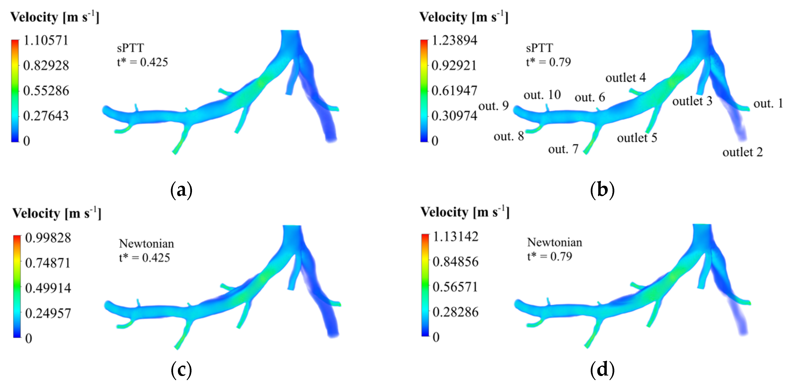
According to Figure 3, the minimum velocity occurs when the dimensionless time, t*, is equal to 0.425 and the maximum one is equal to 0.79, during the diastole and the systolic peak, respectively. The velocity fields in those times instances were retrieved, and they are displayed for the sPTT model (Figure 6a,b) and the Newtonian blood model (Figure 6c,d).

Due to the rise in dynamic pressure, thinner cross-sections have higher velocity magnitudes, such as in the case of the stenosis region and the outlet arteries. This happens for both rheological models. Moreover, in the LAD, it is clear to see that downstream the narrowed vessel, provoked by the stenosis, the velocity gradually decreases to values like the ones registered in the inlet before the bifurcation. Near the walls, friction losses are the cause of the witnessed velocity decreases. In the region near the wall surface before and after outlet 4, there is a stagnant blood flow since the velocity values are near zero. This region is bigger in the Newtonian case and in both time instances.

The sPTT simulations returned higher maximum velocities than the Newtonian model simulations. In fact, the maximum velocity achieved in t* = 0.425 was 9.72% larger and, for the instant t* = 0.79, the maximum velocity was 8.68% higher. It could be concluded that the Newtonian blood model underestimates the maximum velocity that occurs in the stenosis, not accounting for its real impact on blood flow.

3.2. Pressure Fields and Profiles

For the calculation of the FFR, the pressures in the aorta and 20 mm downstream the stenosis are required. The spatial-averaged pressure waveforms at the distal and aortic planes (displayed on Figure 5) are shown in Figure 7 as a function of non-dimensional time, for both sPTT and Newtonian models of blood.

The pressure peak and valley occur approximately in the same instances as the velocity ones. The distal pressure profile reaches lower pressure values, confirming the pressure drop that occurs because of the existence of the stenosis. This happens considering both models for blood. Additionally, the propagation of the pressure pulse from the entrance through the branches of the coronary tree is what causes the observed lag between the minimum and maximum pressure peaks from the aortic to the distal planes. The Newtonian model returned slightly higher pressure values for the aortic and distal plane than the sPTT model since the latter accounts for viscoelastic impacts of blood flow, which lead to lower pressure values.

The pressure fields for the patient are displayed for the minimum and the maximum velocity time instances for the sPTT model (Figure 8a,b) and the Newtonian blood model (Figure 8c,d).

For both rheological models, the maximum pressure reached in t* = 0.425 (Figure 8a,c) is lower than the maximum pressure reached in t* = 0.790 (Figure 8b,d). Since the LCX branch, which is upstream of the stenosis, manages to retain greater pressure values lengthwise, a comparison of the pressure values with the LAD branch denotes the obvious influence the stenosis has on blood flow. The stenosis leads to a pressure drop in the artery that is slowly overturned downstream of the vessel, but the pressure never recovers to the inlet pressure values. This conclusion is supported by Bernoulli’s principle, since the increase in cross-sectional area after the stenosis leads to a pressure increase.

Looking at the pressure contours, it is evident that the pressure decreases in the stenosis area and starts increasing with the downstream distance to the stenosis. However, the pressure considering the viscoelastic model (Figure 8a,b) recuperates over a shorter distance than the Newtonian model (Figure 8c,d). The sPTT simulations returned maximum and minimum pressure values that were lower than the ones using the Newtonian blood model. Quantitatively, in the sPTT case, the maximum pressure reached in t* = 0.425 was 10.12% lower, and the minimum pressure obtained was 55.7% smaller. Similarly, for t* = 0.79, the maximum pressure was 10.92% lower and the minimum pressure obtained was 90.29% smaller.

If the artery had only been numerically studied with the Newtonian model, it could be assumed that the pressure downstream the stenosis would never recuperate and affect the entire circulatory system. Such a conclusion would be misleading and, therefore, a more accurate blood model needs to be computed. Thus, the rheological model to be used in hemodynamic simulations of coronary arteries should take into consideration the viscoelastic property of blood, which is more accurate [20,21,22,23,24].

In the smaller arteries, such as the outlets, the pressure tends to be lower (Figure 8) due to a greater preponderance of viscous strains, the reverse of what occurred with the velocity (Figure 6). To better assess the stenosis impact downstream, the temporal distribution of the spatial-average pressure in each outlet was calculated. These results are displayed considering the sPTT (Figure 9a) and the Newtonian blood models (Figure 9b).

The results of the pressure curves for the sPTT and the Newtonian blood models have similar magnitude and shape. The pressure peaks occur in the same time instances. Before the stenosis, outlet 1 to 3 returned higher pressure values. Then, after the stenosis, its closest exits are outlets 4 and 5, where the recorded pressure is significantly lower in comparison with the first three outlets. The pressure continues to decrease in outlets 6 and 7. The magnitude of pressure is much lower, but it recovers downstream, as is evident by the increase in the pressure values in outlets 8 to 10. Outlet 9 is the furthest from the stenosis, and the pressure values, although larger than the ones of outlets upstream, are still below the initial pressure values. This suggests that the presence of stenosis alters the flow in the arteries and, consequently, of the capacity of the cardiac muscle.

For a better comparison of the results obtained using the two different rheological models, the pressure peaks obtained in each outlet were recovered for both the Newtonian and the sPTT blood models. The pressure values are presented in

Table 6. Maximum outlet pressure for the sPTT and the Newtonian blood models and the relative error values.

Outlet	Maximum Outlet Pressure (sPTT) [Pa]	Maximum Outlet Pressure (Newtonian) [Pa]	Relative Error [%]
Outlet 1	1449.8	1473.5	1.6
Outlet 2	2695.8	2835.0	5.2
Outlet 3	2119.7	2292.0	8.1
Outlet 4	1323.8	1235.4	6.7
Outlet 5	1210.0	1237.4	2.3
Outlet 6	837.4	710.9	15.1
Outlet 7	881.7	1321.3	49.9
Outlet 8	804.0	797.5	0.8
Outlet 9	1746.5	1840.6	5.4
Outlet 10	1233.2	1204.5	2.3

, where the relative error between them is displayed.

The calculated relative error values are diverse, ranging from 0.8% to 49.9% in outlets 8 and 7, respectively. The average relative error is 9.7%. This measure indicates that, since the relative error values are high, the sPTT model must be used in the numerical simulations.

3.3. Non-Invasive FFR

The previous data were used to calculate the temporal and spatial-averaged pressure values for the distal and the aortic planes of the artery to obtain the non-invasive FFR. For both locations, the spatial-average pressure values in different time steps were averaged through a trapezoidal rule. With the ratio of the two values, the FFR value for the patient case was calculated, as well as the relative error to the invasive measurement (

Table 7. Comparison between invasive and non-invasive FFR for the patient case considering the Newtonian and the sPTT blood models.

Blood Model	Invasive FFR	Non-Invasive FFR	er [%]
Newtonian	0.930	0.904	2.74
sPTT		0.934	0.37

).

The non-invasive method captured the hemodynamics of the LCA, given the fact that the computed FFR of the patient is practically equivalent to the invasive FFR, recording a relative error of 0.37%. This error value is much smaller than the one registered in the numerical simulations considering the Newtonian blood model (2.74%). This is due to the fact that the sPTT model considers the viscoelasticity of blood, and it is a more accurate representation of its fluid properties [20,21,22,23,24]. In addition, the use of the Womersley velocity model and the five-element Windkessel flow are essential for reproducing the realistic waveforms of this patient.

Moreover, it is crucial to compare our results with those reported in the recent literature in order to validate the reliability of the implemented method. In a study conducted by Xue et al. (2023), the outlet blood flow conditions were determined based on CT perfusion and outlet diameter, while maintaining a constant pressure at the artery inlet. They assumed blood to be a Newtonian fluid. Like the present work, these authors performed the reconstruction of a coronary artery through 2D images and used clinical information to determine patient-specific boundary conditions. The outlet boundary conditions used were coronary outlet resistance based on the myocardial perfusion territory, extracted from medical imaging of the heart during a cardiac cycle. The mesh used by the authors exceeds 1 × 10⁶ elements, and the software OpenFOAM was used in the numerical simulations. The results showed a relative error of 4.35% and 2.25% between invasive and computed FFR for two patient cases [40]. On the other hand, Gao et al. (2020) utilized a machine learning algorithm to predict the FFR based on CT imaging. The authors created a tree-structured recurrent neural network. The hemodynamic results were obtained through simulations using the finite element method of 1D models of coronary artery trees. The work used outlet pressure and inlet velocity values based on lumped-parameter models. The neural network was trained with 13,000 synthetic coronary trees authors, and eight patient cases were used in the validation stage. The authors achieved an average relative error of 2.85% between invasive and computed FFR for eight patients. Given the low relative error obtained in their work in comparison with state-of-the-art methods, it could be stated that the implemented methods are valid and reliable [41].

4. Conclusions

In this work, a patient-specific geometry of a left coronary artery was generated to perform hemodynamic simulations using computational fluid dynamics, with the objective of calculating the value of the FFR. This parameter is considered the gold standard in the assessment of the severity of a lesion due to the existence of stenosis and the possible need for revascularization. In order to assess the accuracy of the developed numerical model, the non-invasive computed FFR value was compared with the invasively measured one, obtained by the Vila Nova de Gaia/Espinho Hospital Centre.

The geometry of the LCA was modeled through CT scans provided by the CHVNG/E. Using Mimics^® (v20.0) and 3-matic^® (v20.0) software, the geometry under resting conditions was reconstructed. Then, its cross-sectional area was scaled by a factor of 2.04 to replicate the FFR measurement procedure in hyperemic conditions. In order to simulate coronary blood flow, a patient-specific Womersley velocity profile was used as the inlet velocity boundary condition. A simplified Phan-Thien/Tanner rheological model was implemented to model the viscoelastic properties of blood. Moreover, a five-element Windkessel model was modeled as the pressure boundary condition for the outlets of the patient-specific artery geometry. User-defined functions were implemented in ANSYS Fluent^® to consider the previous conditions.

The numerical tool allows for the creation of pressure and velocity domains in the artery along a cardiac cycle, which, due to the accuracy of the chosen boundary conditions and rheological model, would be very approximate to the real-life waveforms of the patients. In addition, this tool allows for the calculation of the non-invasive FFR, a parameter used in clinical settings to assess coronary artery disease and the level of constriction of the coronary arteries. Hence, this work has clinical importance for potentially returning accurate values custom to each patient case, aiding medical doctors in the diagnosis and treatment of their patients with atherosclerosis.

The implemented model produced an FFR value of 0.934 for the patient, which corresponds to a relative error of 0.37% in comparison with the invasive measurement. This error value is lower than the one obtained in the numerical simulations that took into consideration the Newtonian model (2.74%). The results confirm the need to consider the viscoelasticity of blood in realistic blood flow simulations, in alliance with accurate boundary conditions for pressure (Windkessel model) and velocity (Womersley profile).

This work deals with a relevant problem in medical practice since obtaining a computational measure of FFR would aid in clinical practice by replacing invasive FFR procedures. The non-invasive procedure could be a cost-free alternative, with no risk for the patient, which improves the diagnosis and treatment of the disease. After validation with many patient-specific cases, in the future, the final goal of this project is to create software to be used by the medical doctors on-site to obtain an accurate computed FFR avoiding invasive procedures.

Study Limitations

Even though this study returned promising results, some limitations are worth mentioning. Since the 3D geometric model of the patient artery is scaled manually, there can be a loss in patient geometry information, which could be particularly more relevant for higher stenosis severities. Moreover, the authors assumed that the hyperemia condition impacts the vessel in the same constant proportion of 2.04. The ability of the artery to dilate may be different in the stenotic region because of the material properties of the plaque.

Regarding the five-element Windkessel model, it allows for downstream vasculature compliance but ignores coronary artery compliance. The used Windkessel model assumes a Newtonian behavior downstream of the artery, but still considers a viscoelastic model in the artery itself. Since the FFR pressure values are measured around the stenosis in the artery model, where the viscoelastic model was implemented and the corresponding results were very accurate when compared to the invasive measure, this consideration was not relevant.

Moreover, in the coronary artery numerical simulations of the present study, the fluid–structure interaction (FSI) method was not applied since our past works have shown that the implementation of FSI in numerical simulations increased the computational time without improving the accuracy of the hemodynamic results [28]. However, according to the research of Amabili et al. (2020), the human aorta, larger than the coronary artery, possesses a certain degree of flexibility, giving it a pulsatile diameter expansion (10% for a young human aorta) [42].

The myocardial mass used to calculate the compliance parameters corresponds to an average of cadaveric heart weight of healthy adults, and not of live ischemic hearts, because of a lack of data from the hospital and the literature. The knowledge of the myocardial mass index could better assist the authors in using a more accurate myocardial mass value for other patient cases. Moreover, the authors did not consider the possibility of the thickening of arterioles that can occur on ischemic hearts, which would consequently increase their resistance to blood flow.

Evidently, the current study constitutes proof-of-concept, since only one patient has been studied. Thus, in the near future and before clinical use, the numerical software must be further validated with many patient cases, with different stenosis severities in separate locations of the coronary artery.