Two Combinatorial Algorithms for the Constrained Assignment Problem with Bounds and Penalties

Abstract

In the paper, we consider a generalization of the classical assignment problem, which is called the constrained assignment problem with bounds and penalties (CA-BP). Specifically, given a set of machines and a set of independent jobs, each machine has a lower and upper bound on the number of jobs that can be executed, and each job must be either executed on some machine with a given processing time or rejected with a penalty that we must pay for. No job can be executed on more than one machine. We aim to find an assignment scheme for these jobs that satisfies the constraints mentioned above. The objective is to minimize the total processing time of executed jobs as well as the penalties from rejected jobs. The CA-BP is related to some practical applications such as edge computing, which involves selecting tasks and processing them on the edge servers of an internet network. As a result, a motivation of this study is to improve the efficiency of internet networks by limiting the lower bound of the number of objects processed by each edge server. Our main contribution is modifying the previous network flow algorithms to satisfy the lower capacity constraints, for which we design two exact combinatorial algorithms to solve the CA-BP. Our methodologies and results bring novel perspectives into other research areas related to the assignment problem.

1. Introduction

To address the substantial increase in mobile data traffic, edge computing, which refers to selecting tasks and processing them on the edge servers of the internet network [1], has emerged as a compelling solution to enhance computing performance. This approach involves the deployment of cloud computing services at the edges of the network, offering the potential for significant improvements [2]. Edge computing can effectively overcome the deficiencies of core network congestion and high latency that are commonly observed in conventional cloud computing systems.

The Cloud–Edge Collaborative Computing Framework (CECCF) [2] is a computing framework where the first step performs edge computing and the second transfers the remaining tasks to the cloud computing center for further processing. In most cases in the CECCF, the edge servers can be seen as machines. The objective of task offloading in the CECCF entails the strategic selection of specific tasks for execution by edge servers and delegating the remaining tasks to be processed by cloud computing centers, so as to minimize the total cost of processing tasks on the edge servers plus the cost of processing the remaining tasks in the cloud computing center.

1.1. Model Description

In order to use the internet network edges more efficiently, it is usually expected that the number of objects served by any edge server will exceed a certain number. Inspired by this thinking, we model the task offloading problem driven by the CECCF as a constrained assignment problem with bounds and penalties (CA-BP). Treating the cost of processing any task on the cloud computing center in the above context as a penalty, the CA-BP is modeled as follows. The input of the CA-BP consists of a set $M=\{M_1,M_2,\dots ,M_m\}$ of m machines (edge servers) with two integer functions $l,u:M\to Z^{+}$, and a set $J=\{J_1,J_2,\dots ,J_n\}$ of n jobs (computation tasks) with a function $p:J\to Z_0^{+}$. It is necessary for each machine $M_i\in M$ to receive at least $l_i$ and at most $u_i$ jobs from J to execute. Each job $J_j\in J$ must be either executed on some machine $M_i\in M$ with its processing time $c_{ij}$ or rejected (executed by the cloud computing center) and given a penalty (computing cost) $p_j$ that we must pay for. No job in J can be executed on more than one machine. We aim to find an assignment scheme of these n jobs that satisfies the aforementioned constraints. The objective is to minimize the total processing time of executed jobs as well as the penalties from rejected jobs.

1.2. Literature Review

The assignment problem (AP) is one of the well-known combinatorial optimization problems, which has many wide applications in real life [3]. This assignment problem was first raised in 1952 by Votaw and Orden [4]. Subsequently, Kuhn [5] in 1955 presented the Hungarian method to solve the assignment problem and examined the actual solutions of the assignment problem and its variations. In the past six decades, the assignment problem has been deeply studied in the literature  [6,7,8,9].

According to the difference in the numbers of jobs and machines, assignment problems can be generally divided into two categories, namely one-to-one assignment problems (OTO-APs) and one-to-many assignment problems (OTM-APs) [3]. The OTO-AP is described as follows. Given a factory that has n machines and an order to process n jobs, each machine must receive exactly one job, and each job is only executed on one machine with its given processing time. An assignment scheme to minimize the total processing time is thus needed. Another kind of assignment problem is the OTM-AP. In this problem, the number of jobs and the number of machines are no longer equal, and a machine can execute multiple jobs.

The OTO-AP is mathematically related to the weighted bipartite matching problem in graph theory [3], and many efficient algorithms [3,5,10] have been presented to solve this problem, among which the most famous is the Hungarian method proposed in [5]. The OTM-AP can be viewed as a scheduling problem [11], which has been solved by the shortest processing time first (SPT) algorithm [12]. Moreover, by applying the circular flow method, the OTM-AP can be solved in polynomial time [10,13]. In addition, a variation of the OTM-AP is to minimize the maximum processing time of the machines. This problem and other related problems have been considered extensively in the literature [14,15,16,17].

With continuous research on the assignment problem, researchers have found that when the processing times of some jobs are very long, no matter which machines the jobs are assigned to for processing, it will cause the objective function value to become very large. As was surveyed by Shabtay et al. [18], in many cases, processing all jobs may not be a good strategy. A strategy which leads to penalties for rejecting some jobs would still have an acceptable total benefit; i.e., this scheme for n jobs would be better.

Based on the aforementioned idea, Bartal et al. [19] in 2000 first proposed the parallel machines scheduling problem with rejection, which is modeled as follows. Given a set $M=\{M_1,\dots ,M_m\}$ of m parallel (identical) machines and a set $J=\{J_1,\dots ,J_n\}$ of n jobs, each job $J_j$ has a processing time $c_j>0$ and a penalty $p_j\ge 0$. The model is tasked with assigning these n jobs to m machines for execution, and the objective is to minimize the maximum processing time of machines as well as the penalties from rejected jobs. Bartal et al. [19] designed an online algorithm with the best-possible competitive ratio $\frac{\sqrt{5}+3}{2}$ for the online version and presented a polynomial time approximation scheme (PTAS) for the offline version. Following this pioneering work, scheduling problems with rejection have been studied extensively in the literature [20,21,22,23,24,25].

1.3. Main Contributions

The main contributions of this paper are as follows: (1) We are the first to attempt to model the task offloading problem in cloud–edge collaborative computing as the CA-BP, and based on our modeling method, many related task-offloading problems in cloud–edge collaborative computing can be solved. (2) Using a strategy that satisfies the lower capacity constraints first, we modify several previous network flow algorithms to match the capacity constraint with the upper and lower bounds. (3) Using the modified network flow algorithms in (2), we design two exact combinatorial algorithms to solve the CA-BP.

The remainder of this paper is organized as follows. In Section 2, we present some terminologies and fundamental lemmas to ensure the correctness of our algorithms. In Section 3, we design two exact combinatorial algorithms to solve the CA-BP. In Section 4, we present our conclusion and further directions.

2. Terminologies and Fundamental Lemmas

In this section, we provide some terminologies, notations, and fundamental lemmas in order to verify the algorithms used for solving the CA-BP.

For convenience, we denote $I=(J,M;l,u;c,p)$ as an instance of the CA-BP, where $M=\{M_1,M_2,\dots ,M_m\}$ is a set of m machines and $J=\{J_1,J_2,\dots ,J_n\}$ is a set of n jobs. Each machine $M_i\in M$ must execute at least $l_i$ and at most $u_i$ jobs from J, and each job $J_j\in J$ must be either executed on some machine $M_i\in M$ within its processing time $c_{ij}$ or rejected with a penalty $p_j$ that we must pay for. No job can be executed on more than one machine.

For an arc set A and an element e, we use the notation $e\in A$ to denote that the element e belongs to the set A. Given a network (directed graph) N with a source s and a sink t, we restate some definitions and problems in [26]. Note that from now on the network refers to the directed graph, unlike the “network” in the Abstract and Introduction.

Definition 1.

Given a network $N=(V,A;u;s,t)$ with a source s, a sink t, and a capacity function $u:A\to Z^{+}$, we define an $(s,t)$-flow f (in N) to be a function $f:A\to R_0^{+}$ satisfying the following three conditions:

(1) 

The capacity constraint: for each arc $e\in A$, we have $0\le f\left(e\right)\le u\left(e\right)$, where $f\left(e\right)$ is called the flow value of this arc e;

(2) 

The flow conservation: for each vertex $v\in V\backslash \{s,t\}$, we have ${\sum }_{e\in {\delta }^{+}\left(v\right)}f\left(e\right)={\sum }_{e\in {\delta }^{-}\left(v\right)}f\left(e\right)$, where ${\delta }^{+}\left(v\right)=\{(v,x)$|$(v,x)\in A\}$ and ${\delta }^{-}\left(v\right)=\{(y,v)$|$(y,v)\in A\}$;

(3) 

For the source s, we have $v\left(f\right)={\sum }_{e\in {\delta }^{+}\left(s\right)}f\left(e\right)-{\sum }_{e\in {\delta }^{-}\left(s\right)}f\left(e\right)\ge 0$.

We call $v\left(f\right)$ the value of an $(s,t)$-flow f. In addition, for any $(s,t)$-flow f in a network $N=(V,A;u,b;s,t)$, where $b:A\to R^{+}$ is a unit cost function, we define the cost of flow f as $b\left(f\right)={\sum }_{e\in A}b\left(e\right)f\left(e\right)$. Furthermore, if the value $f\left(e\right)$ is an integer for each $e\in A$, this $(s,t)$-flow f is called an integer $(s,t)$-flow in N.

Problem 1

(the maximum flow problem). Given a network $N=(V,A;u;s,t)$ with a capacity function $u:A\to R^{+}$, the maximum flow problem is to find an $(s,t)$-flow f in N. The objective is to maximize the value $v\left(f\right)$=${\sum }_{e\in {\delta }^{+}\left(s\right)}f\left(e\right)-{\sum }_{e\in {\delta }^{-}\left(s\right)}f\left(e\right)$ among all $(s,t)$-flows in N.

Problem 2

(the minimum-cost flow problem). Given a network $N=(V,A;u;b;s,t)$ and a positive integer k, where $u:A\to R^{+}$ is a capacity function and $b:A\to R^{+}$ is a unit cost function, the minimum-cost flow problem is to find an $(s,t)$-flow f with value $v\left(f\right)=k$; the objective is to minimize the cost $b\left(f\right)={\sum }_{e\in A}b\left(e\right)f\left(e\right)$ among all $(s,t)$-flows with value k in N.

3. Constrained Assignment Problem with Bounds and Penalties

In this section, we consider the constrained assignment problem with bounds and penalties (CA-BP). The objective is to minimize the total processing times of executed jobs as well as the penalties from rejected jobs. Without loss of generality, we assume that $n\ge m$; otherwise, there is no feasible solution to the CA-BP.

Given an instance $I=(J,M;l,u;c,p)$ of the CA-BP, we use variables $\left\{x_{ij}\right|i=1,2,\dots ,m$ and $j=1,2,\dots ,n\}$ simply as a scheme ${\left\{x_{ij}\right\}}_{mn}$, to represent an execution of n jobs on m machines, where a variable $x_{ij}=1$ indicates the job $J_j$ to be executed on that machine $M_i$, and otherwise, $x_{ij}=0$ for any $i\in \{1,2,\dots ,m\}$ and $j\in \{1,2,\dots ,n\}$. Then, we may obtain the linear integer programming (IP) to determine the CA-BP as follows:      $\left(IP\right)minz={\sum }_{i=1}^m{\sum }_{j=1}^n{c}_{ij}{x}_{ij}+{\sum }_{j=1}^n{p}_j(1-{\sum }_{i=1}^m{x}_{ij})$

$$\begin{array}{c}\mathrm{s}.\mathrm{t}.\left\{\begin{array}{cccc}\hfill & \sum _{i=1}^m{x}_{ij}\le 1\hfill & \hfill \mathrm{f}\mathrm{o}\mathrm{r}& j=1,2,\dots ,n\hfill \\ \hfill & l_i\le \sum _{j=1}^n{x}_{ij}\le u_i\hfill & \hfill \mathrm{f}\mathrm{o}\mathrm{r}& i=1,2,\dots ,m\hfill \\ \hfill & x_{ij}\in \{0,1\}\hfill & \hfill \mathrm{f}\mathrm{o}\mathrm{r}& i=1,2,\dots ,m\mathrm{a}\mathrm{n}\mathrm{d}j=1,2,\dots ,n,\hfill \end{array}\right.\hfill \end{array}$$

(1)

where the first constraint indicates that each job is assigned on at most one machine to be executed; i.e., no job can be executed on more than one machine. The second constraint indicates that each machine $M_i$ must execute at least $l_i$ and at most $u_i$ jobs from J.

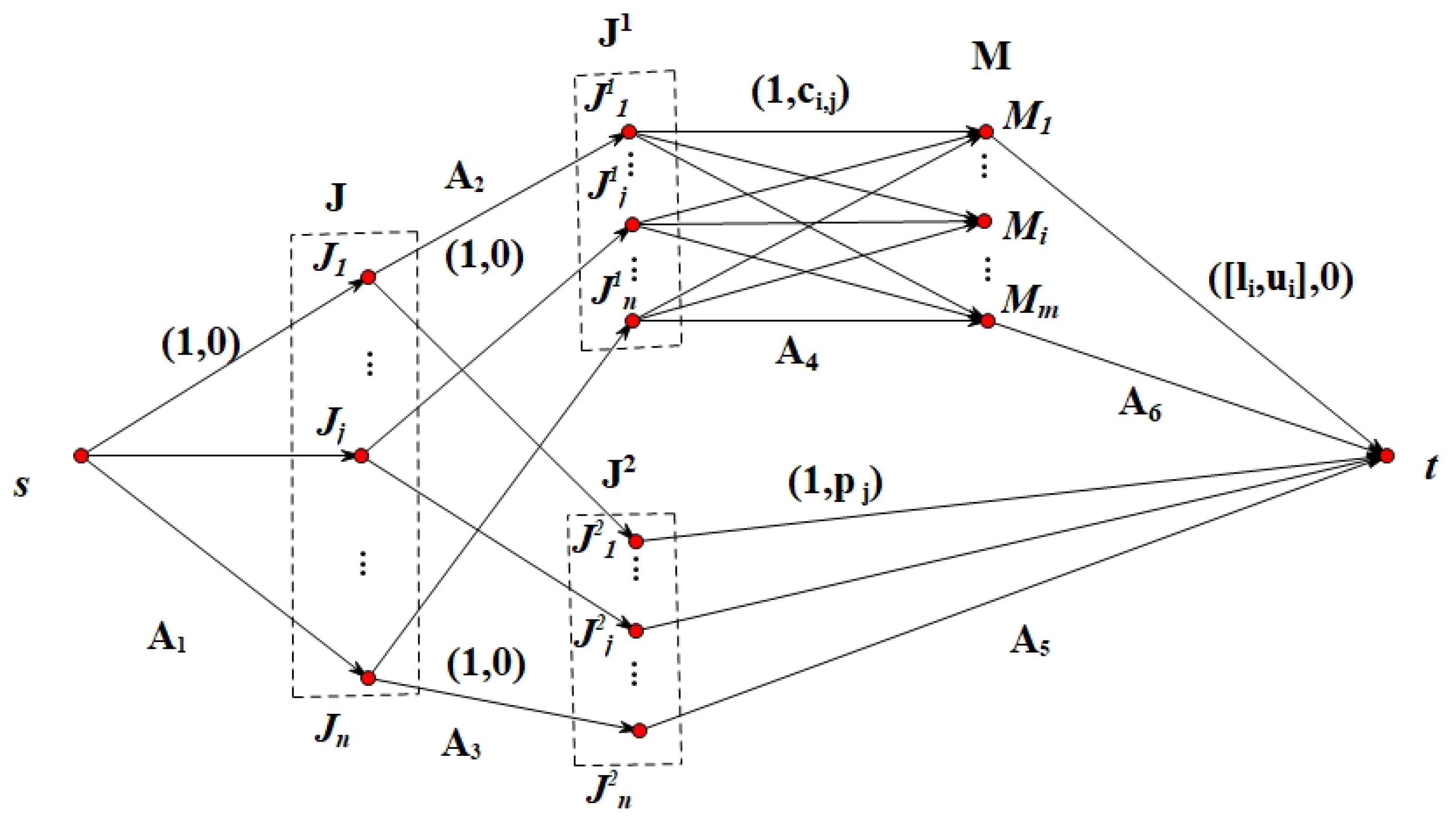
In order to optimally solve the CA-BP, and equivalently the linear integer programming (IP), we intend to transfer the CA-BP to the minimum-cost flow problem on a special network constructed in the following, where the flow value of each arc in such a problem must be between a lower bound and an upper bound. Figure 1 roughly illustrates the process of this transformation.

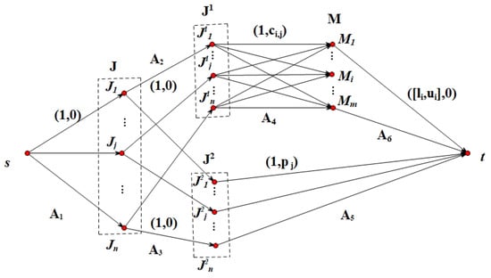
Figure 1. Construction of a network $N=(V,A;l,u;b;s,t)$.

Given an instance $I=(J,M;l,u;c,p)$ of the CA-BP, we can construct a network $N=(V,A;l,u;b;s,t)$ in the following ways. Denote $V=J\cup J^1\cup J^2\cup M\cup \{s,t\}$, where s and t are two special vertices; $J^1=\{J_1^1,J_2^1,\dots ,J_n^1\}$ and $J^2=\{J_1^2,J_2^2,\dots ,J_n^2\}$ are two sets of vertices copied from the set $J=\{J_1,J_2,\dots ,J_n\}$, respectively; and $A=A_1\cup A_2\cup A_3\cup A_4\cup A_5\cup A_6$, where $A_1=\left\{(s,J_j)\right|J_j\in J\}$, $A_2=\left\{(J_j,J_j^1)\right|j=1,2\dots ,n\}$, $A_3=\left\{(J_j,J_j^2)\right|j=1,2\dots ,n\}$, $A_4=\left\{(J_j^1,M_i)\right|J_j^1\in J^1,M_i\in M$}, $A_5=\left\{(J_j^2,t)\right|J_j^2\in J^2\}$, $A_6=\left\{(M_i,t)\right|M_i\in M\}$. We may define lower and upper capacities and unit costs on these arcs as follows. For each arc $e\in A_1\cup A_2\cup A_3\cup A_4\cup A_5$, let the lower capacity $l\left(e\right)=0$ and the upper capacity $u\left(e\right)=1$. For each arc $(M_i,t)\in A_6$, let $l(M_i,t)=l_i$ and $u(M_i,t)=u_i$. At the same time, let the unit cost $b(J_j^1,M_i)=c_{ij}$ for each arc $(J_j^1,M_i)\in A_4$, the unit cost $b(J_j^2,t)=p_j$ for each arc $(J_j^2,t)\in A_5$, and $b\left(e\right)=0$ for each arc $e\in A_1\cup A_2\cup A_3\cup A_6$. In addition, if there exists an $(s,t)$-flow $f:A\to R_0^{+}$ in this network $N=(V,A;l,u;b;s,t)$, to satisfy $l\left(e\right)\le f\left(e\right)\le u\left(e\right)$ for each arc $e\in A$, we call this flow f a bounded $(s,t)$-flow in N.

Using the aforementioned construction, we obtain the following key lemma.

Lemma 1.

Given an instance $I=(J,M;l,u;c,p)$ of the CA-BP, we can construct a network $N=(V,A;l,u;b;s,t)$ as mentioned above, such that there is a feasible solution with cost z on the instance I if and only if there is an integer-bounded $(s,t)$-flow f of value $v\left(f\right)=n$ in N, where the cost is $b\left(f\right)=z$.

Proof. 

(Necessity) Suppose that there is a feasible scheme ${\left\{x_{ij}\right\}}_{mn}$ with cost z for the linear integer programming ($IP$). We construct an integer $(s,t)$-flow f in N as follows. For every $x_{ij}$ in ${\left\{x_{ij}\right\}}_{mn}$, if $x_{ij}=1$, let $f(s,J_j)=1$, $f(J_j,J_j^1)=1$, $f(J_j^1,M_i)=1$, $f(J_j,J_j^2)=0$, and $f(J_j^2,t)=0$; otherwise, let $f(s,J_j)=1$, $f(J_j,J_j^1)=0$, $f(J_j^1,M_i)=0$, $f(J_j,J_j^2)=1$, and $f(J_j^2,t)=1$. For each $M_i\in M$, let $f(M_i,t)={\sum }_{j\in J}{x}_{ij}$, which implies that $l_i\le f(M_i,t)={\sum }_{j\in J}{x}_{ij}\le u_i$. Using this construction, we easily obtain that f is an integer-bounded $(s,t)$-flow of value n in N, where the cost is $b\left(f\right)=z$.

(Sufficiency) Suppose that there exists an integer-bounded $(s,t)$-flow f with value n and cost $b\left(f\right)$ in N. It is easy to see that $f(s,J_j)=1$ for each arc $(s,J_j)\in A_1$, implying that $f(J_j,J_j^1)+f(J_j,J_j^2)=1$, and $f\left(e\right)\in \{0,1\}$ for each arc $e\in A\setminus A_6$. We construct a scheme ${\left\{x_{ij}\right\}}_{mn}$ for the linear integer programming (IP) as follows. For each arc $(J_j^1,M_i)\in A_4$, if $f(J_j^1,M_i)=1$, denote $x_{ij}=1$; otherwise, denote $x_{ij}=0$. Using this construction, for each $M_i\in M$, we have ${\sum }_{j=1}^n{x}_{ij}=f(M_i,t)$, implying that $l_i\le {\sum }_{j=1}^n{x}_{ij}\le u_i$. This easily shows that the scheme ${\left\{x_{ij}\right\}}_{mn}$ is a feasible solution to the linear integer programming ($IP$), i.e., a feasible solution for the CA-BP, where the cost is $z=b\left(f\right)$.

This completes the proof of the lemma.  □

Using Lemma 1, we easily obtain the following.

Corollary 1.

The CA-BP has an optimal solution with cost z if and only if there exists a minimum-cost integer-bounded $(s,t)$-flow f of value n in N (mentioned above), where the cost $b\left(f\right)=z$.

In order to find the minimum-cost integer-bounded $(s,t)$-flow in N, we need the following definitions.

Definition 2

(The residual network). Suppose that f is a bounded $(s,t)$-flow with value k in the network $N=(V,A;l,u;b;s,t)$. The residual network $N_f=(V,A_f;u_f;s,t)$ of N, with respect to f, is constructed in the following way: (1) At the beginning, let $A_f=Ø$. (2) For each arc $(x,y)\in A$, we add two residual arcs $(x,y)$ and $(y,x)$ to $A_f$, where the residual capacities are $u_f(x,y)=u(x,y)-f(x,y)$ and $u_f(y,x)=f(x,y)-l(x,y)$. (3) Then, we delete arcs in $A_f$ whose residual capacities are 0.

Definition 3

(The incremental network). Suppose that f is a bounded $(s,t)$-flow with value k in the network $N=(V,A;l,u;b;s,t)$. The incremental network $N_f^{\prime }=(V,A_f^{\prime };u_f^{\prime };b_f^{\prime };s,t)$ of N, with respect to f, is constructed in the following way: (1) At the beginning, let $A_f^{\prime }=Ø$. (2) For each arc $(x,y)\in A$, we add two incremental arcs $(x,y)$ and $(y,x)$ to $A_f^{\prime }$, where the incremental capacities $u_f^{\prime }(x,y)=u(x,y)-f(x,y)$, $u_f^{\prime }(y,x)=f(x,y)-l(x,y)$ and the unit incremental costs $b_f^{\prime }(x,y)=b(x,y)$, $b_f^{\prime }(y,x)=-b(x,y)$. (3) Then, we delete all arcs in $A_f^{\prime }$ whose incremental capacities are 0.

Similarly, to solve the minimum-cost flow problem, we obtain a result for the bounded flow as follows. The method of proof is similar to Theorem 12.1 in [10]; we present its proof in detail for completeness.

Lemma 2.

Let f be an integer-bounded $(s,t)$-flow with value n in the network $N=(V,A;l,u;b;s,t)$ mentioned above. Then, f is a minimum-cost integer-bounded $(s,t)$-flow with value n if and only if the incremental network $N_f^{\prime }=(V,A_f^{\prime };u_f^{\prime };b_f^{\prime };s,t)$ has no negative directed cycle with respect to the incremental cost function $b_f^{\prime }(·)$.

Proof. 

(Necessity) Suppose, to the contrary, that there is a directed cycle $\mathcal{C}$ with a negative cost in the incremental network $N_f^{\prime }=(V,A_f^{\prime };u_f^{\prime };b_f^{\prime };s,t)$. We can augment the current flow f along $\mathcal{C}$ by some value $\theta \in Z^{+}$ to obtain a new flow $f^{\prime }$ with value n. According to the construction of the incremental network, the augment process does not violate the lower and upper bound constraints, so $f^{\prime }$ is an integer-bounded $(s,t)$-flow with value n. Since the cost of $\mathcal{C}$ is negative, we have $b\left(f^{\prime }\right)<b\left(f\right)$, which contradicts the fact that f is a minimum-cost integer-bounded $(s,t)$-flow.

(Sufficiency) Assume that every directed cycle $\mathcal{C}$ in the incremental network $N_f^{\prime }$ has a non-negative cost. For each arc $(y,z)\in A$ and $(z,y)\in A_f^{\prime }$, we define ${\chi }^{\mathcal{C}}\in R^{\left|A\right|}$ by the following:

$${\chi }^{\mathcal{C}}(y,z):=\left\{\begin{array}{cccc}& 1\hfill & \hfill \mathrm{if}& \mathcal{C}\mathrm{passes}\mathrm{through}(y,z)\hfill \\ & -1\hfill & \hfill \mathrm{if}& \mathcal{C}\mathrm{passes}\mathrm{through}(z,y)\hfill \\ & 0\hfill & \hfill \mathrm{if}& \mathcal{C}\mathrm{passes}\mathrm{through}\mathrm{neither}(y,z)\mathrm{nor}(z,y)\hfill \end{array}\right.$$

Let $f^{\prime }$ be another feasible integer-bounded $(s,t)$-flow. Then, $\tilde{f}\triangleq f^{\prime }-f$ is a feasible circular flow, and we have

$$\tilde{f}=\sum _{q=1}^{\left|A\right|}{\xi }_q{\chi }^{{\mathcal{C}}_q},$$

where ${\mathcal{C}}_1,\dots ,{\mathcal{C}}_{\left|A\right|}$ are directed cycles in the incremental network $N_f^{\prime }$, and ${\xi }_1,\dots ,{\xi }_{\left|A\right|}>0$. That is, the flow $\tilde{f}$ can be decomposed into flows on some circles. Therefore,

$$b\left(f^{\prime }\right)-b\left(f\right)=b(f^{\prime }-f)=\sum _{q=1}^{\left|A\right|}{\xi }_{q}b\left({\mathcal{C}}_q\right)\ge 0.$$

Since every directed cycle ${\mathcal{C}}_q$ has a non-negative total cost $b\left({\mathcal{C}}_q\right)$, we have $b\left(f^{\prime }\right)\ge b\left(f\right)$.

This completes the proof of the lemma.  □

According to the aforementioned results, we can use the following strategies to find a minimum-cost integer-bounded $(s,t)$-flow with value n in the network $N=(V,A;l,u;b;s,t)$:

(1)

Firstly, we determine an integer $(s,t)$-flow with value ${\sum }_{i=1}^n{l}_i$ in N to satisfy the lower bounds of arc capacities.

(2)

Secondly, we augment the flow obtained in (1) to a minimum-cost integer-bounded $(s,t)$-flow with value n in the network $N=(V,A;l,u;b;s,t)$.

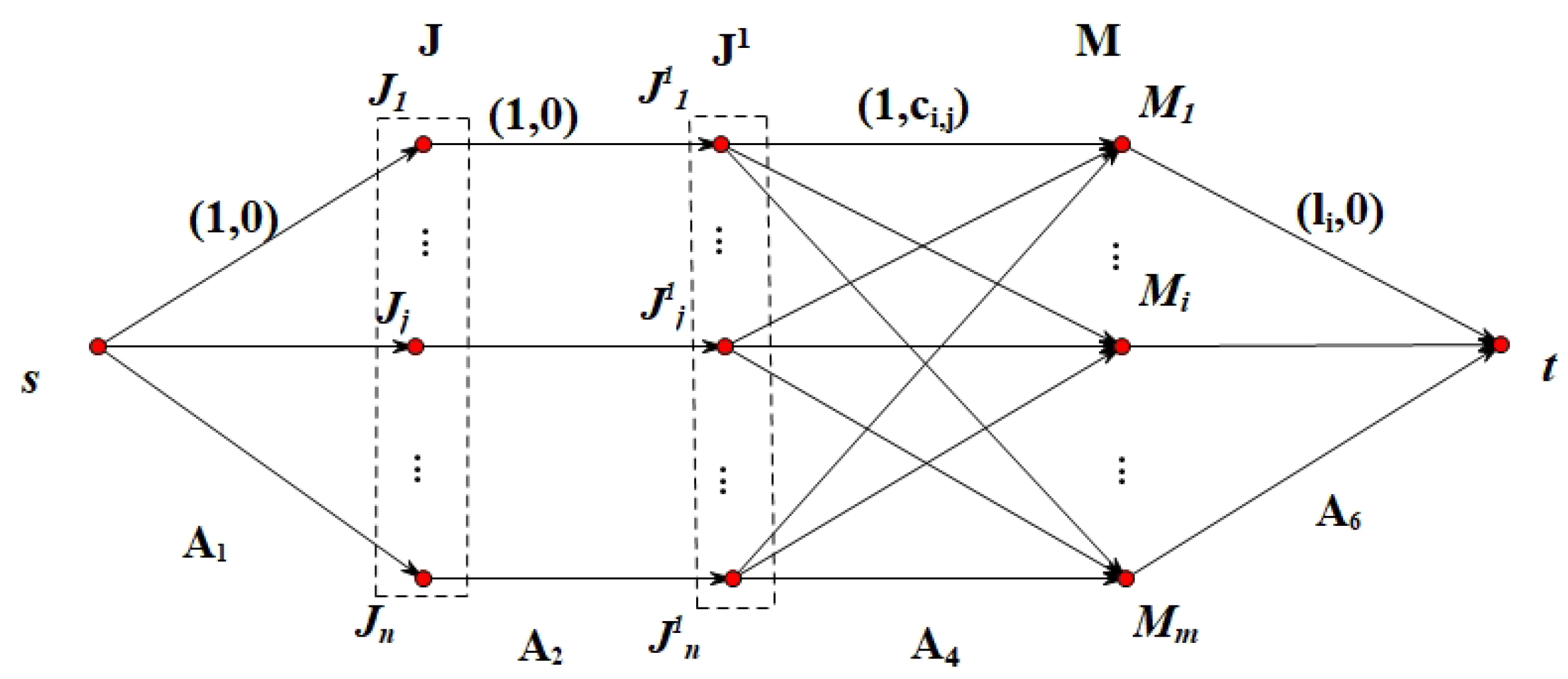
To solve stage (1), we construct another network $N_1=(V^{\prime },A^{\prime };u_1,b;s,t)$ from the network $N=(V,A;l,u;b;s,t)$, where $V^{\prime }=V\setminus J_2$, $A^{\prime }=A_1\cup A_2\cup A_4\cup A_6$, and the capacity is $u_1(M_i,t)=l_i$ for each $(M_i,t)\in A_6$ and $u_1\left(e\right)=1$ for each $e\in A_1\cup A_2\cup A_4$. This process is shown in Figure 2. In this network $N_1=(V^{\prime },A^{\prime };u_1,b;s,t)$, we can use the Edmonds–Karp algorithm [27] in polynomial time to find an integer $(s,t)$-flow with value ${\sum }_{i=1}^n{l}_i$.

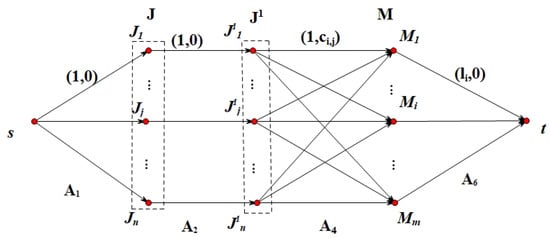
Figure 2. Construction of a network $N_1=(V^{\prime },A^{\prime };u_1,b;s,t)$.

Using Lemma 2 and the two aforementioned stages, we design a combinatorial algorithm, denoted by ${\mathcal{A}}_{CA-B{P}_1}$ (Algorithm 1), to solve the CA-BP.

Algorithm 1: ${\mathcal{A}}_{CA-B{P}_1}$

Input: An instance $I=(J,M;l,u;c,p)$ of the CA-BP. Output: A scheme ${\left\{x_{ij}\right\}}_{mn}$ of the linear integer programming (IP) with respect to I, or “no solution”. Begin    Step 1. If (${\sum }_{i=1}^m{l}_i>n$), then    Output “no solution”, and STOP. Step 2. For the given instance $I=(J,M;l,u;c,p)$ of the CA-BP, as mentioned above, first construct a network $N=(V,A;l,u;b;s,t)$, and then construct another network $N_1=(V^{\prime },A^{\prime };u_1,b;s,t)$. Step 3. Use the Edmonds–Karp algorithm [27] in the network $N_1=(V^{\prime },A^{\prime };u_1,b;s,t)$ to produce an integer $(s,t)$-flow $f_1$ with value $v\left(f_1\right)={\sum }_{i=1}^m{l}_i$. Step 4. From the $(s,t)$-flow $f_1$ in $N_1$, construct an integer $(s,t)$-flow f with value $v\left(f\right)={\sum }_{i=1}^m{l}_i$ in N as follows: (1) For each arc $e\in A_1\cup A_2\cup A_4\cup A_6$ ($=A^{\prime }$), let $f\left(e\right)=f_1\left(e\right)$. (2) For each arc $e\in A_3\cup A_5$ ($=A\backslash A^{\prime }$), let $f\left(e\right)=0$. Step 5. While ($v\left(f\right)<n$) perform the following:    5.1 For the current integer $(s,t)$-flow f in N, construct the corresponding residual network $N_f=(V,A_f;u_f;s,t)$ by Definition 2;    5.2 Find a directed path $P_{st}$ with the least arcs on the residual network $N_f=(V,A_f;u_f;s,t)$, and augment the current integer-bounded $(s,t)$-flow f along $P_{st}$ by the minimum augmentation capacity. Step 6. For the current integer-bounded $(s,t)$-flow f with value n in N, construct the corresponding incremental network $N_f^{\prime }=(V,A_f^{\prime };u_f^{\prime };b_f^{\prime };s,t)$ by Definition 3. Apply the minimum mean cycle algorithm [28] to produce a minimum mean cycle C in $N_f^{\prime }$ with respect to function $b_f^{\prime }(·)$. Step 7. If ($b_f^{\prime }\left(C\right)<0$), then    Along this minimum mean cycle C, augment this integer-bounded $(s,t)$-flow f to a new integer-bounded $(s,t)$-flow f by the minimum augmentation capacity, and go to Step 6. Step 8. From the $(s,t)$-flow f, construct a scheme ${\left\{x_{ij}\right\}}_{mn}$ as follows: for each $i=1,2,\dots ,m$ and $j=1,2,\dots ,n$, if $f(J_j^1,M_i)=1$, choose $x_{ij}=1$; otherwise, $x_{ij}=0$. Step 9. Output this scheme ${\left\{x_{ij}\right\}}_{mn}$. End

Using the algorithm ${\mathcal{A}}_{CA-B{P}_1}$, we obtain the following result.

Theorem 1.

The algorithm ${\mathcal{A}}_{CA-B{P}_1}$ is an optimal algorithm to solve the CA-BP, and it runs in time $O(m^3{n}^{5}log(m+n))$, where m and n are the numbers of machines and jobs, respectively.

Proof. 

By Lemma 2, it is easy to see that the algorithm ${\mathcal{A}}_{CA-B{P}_1}$ can optimally solve the CA-BP. In the first stage (Steps 1–5) of the algorithm ${\mathcal{A}}_{CA-B{P}_1}$, we can use the Edmonds–Karp algorithm [27] to find an integer $(s,t)$-flow with value n in time $O\left(m^2{n}^3\right)$, where m and n are the numbers of machines and jobs, respectively. Furthermore, in the second stage (Steps 6–7) of the algorithm ${\mathcal{A}}_{CA-B{P}_1}$, we can use the minimum mean cycle algorithm [28] to find a minimum-cost $(s,t)$-flow with value n in time $O(m^3{n}^{5}log(m+n))$. To sum up, the total running time of the algorithm ${\mathcal{A}}_{CA-B{P}_1}$ is $O(m^3{n}^{5}log(m+n))$.

This completes the proof of the theorem.  □

To facilitate the understanding of the algorithm ${\mathcal{A}}_{CA-B{P}_1}$, we give the following small example $\mathcal{E}$: m = 2, n = 4. The penalty costs are $p_1=3$, $p_2=2$, $p_3=2$, and $p_4=1$, respectively. The processing time for each job is given in Table 1, and the upper and lower bound constraints for each machine are given in Table 2. Now, we consider the processes of applying algorithm ${\mathcal{A}}_{CA-B{P}_1}$ to this example.

Table 1. Processing time for example $\mathcal{E}$.

	${\mathit{J}}_1$	${\mathit{J}}_2$	${\mathit{J}}_3$	${\mathit{J}}_3$
$M_1$	3	1	1	2
$M_2$	1	2	1	3

Table 2. Upper and lower bound constraints for example $\mathcal{E}$.

i	1	2
$l_i$	1	0
$u_i$	3	2

Applying Steps 1–4 of the algorithm ${\mathcal{A}}_{CA-B{P}_1}$, an integer $(s,t)$-flow f with value $v\left(f\right)=1$ in N can be found as follows: (a) $f(s,J_2)=f(J_2,J_2^1)=f(J_2^1,M_1)=f(M_1,t)=1$; (b) $f\left(e\right)=0$ for each remaining arc $e\in N$. Then, Steps 5–7 augment the current integer $(s,t)$-flow f, and a new integer-bounded $(s,t)$-flow f with value $v\left(f\right)=4$ in N is produced as follows: (1) $f(s,J_1)=f(J_1,J_1^1)=f(J_1^1,M_2)=f(M_2,t)=1$; (2) $f(s,J_2)=f(J_2,J_2^1)=f(J_2^1,M_1)=1$; (3) $f(s,J_3)=f(J_3,J_3^1)=f(J_3^1,M_1)=1$; (4) $f(s,J_4)=f(J_4,J_4^2)=f(J_4^2,t)=1$; (5) $f(M_1,t)=2$; (6) $f\left(e\right)=0$ for each remaining arc $e\in N$. According to the flow f, a scheme ${\left\{x_{ij}\right\}}_{23}$ with the optimal value $z=4$ is found, where the optimal scheme ${\left\{x_{ij}\right\}}_{23}$ is to reject job $J_4$ and to execute job $J_1$ on machine $M_2$ and jobs $J_2$ and $J_3$ on machine $M_1$.

On the other hand, by further analyzing the construction of N, we hope to reduce the complexity of the algorithm ${\mathcal{A}}_{CA-B{P}_1}$ to solve the CA-BP. Therefore, according to the other algorithms for solving the minimum-cost flow problem, we intend to design another algorithm to resolve the CA-BP. Using similar arguments as in [26], we obtain the following result.

Lemma 3.

Let f be a minimum-cost bounded $(s,t)$-flow with value k $(<n)$ in the network $N=(V,A;l,u;b;s,t)$ as mentioned above, where $f(M_i,t)\ge l_i$ for each $(M_i,t)\in A_6$. Let $P_{st}$ be the shortest directed s–t path in $N_f^{\prime }$ with respect to the cost function $b_f^{\prime }(·)$,and $f^{\ast }$ be an $(s,t)$-flow obtained when augmenting f along $P_{st}$ by at most the minimum augmentation capacity θ on $P_{st}$, that is,

$$f_{ij}^{\prime }=\left\{\begin{array}{cccc}& \theta \hfill & \hfill \mathrm{if}& (y_i,y_j)\in A\left(P_{st}\right)\hfill \\ & 0\hfill & \hfill \mathrm{if}& (y_i,y_j)\notin A\left(P_{st}\right)\hfill \end{array}\right.$$

Then, $f^{\ast }=f+f^{\prime }$ is a minimum-cost bounded $(s,t)$-flow with value $k+\theta$.

Proof. 

It is easy to see that $f^{\ast }=f+f^{\prime }$ is a feasible bounded $(s,t)$-flow with value $k+\theta$ in N. Considering the incremental network $N_{f+f^{\prime }}^{\prime }$, the reverse of arc e must be in $P_{st}$ for any arc $e\in A_{f+f^{\prime }}^{\prime }\backslash A_f^{\prime }$.

Suppose, on the contrary, that $f^{\ast }\triangleq f+f^{\prime }$ is not a minimum-cost bounded $(s,t)$-flow. As we know from Lemma 2, there must be a negative cycle $\mathcal{C}$ in $N_{f^{\ast }}^{\prime }$. Since f is the minimum-cost bounded $(s,t)$-flow with value k in the network N, we obtain that $\mathcal{C}$ must contain some arcs $(y_{i_1},y_{j_1})$, $(y_{i_2},y_{j_2})$, ⋯, $(y_{i_{l^{\ast }}},y_{j_{l^{\ast }}})$ in $A_{f+f^{\prime }}^{\prime }\backslash A_f^{\prime }$, corresponding to arcs $(y_{j_1},y_{i_1})$, $(y_{j_2},y_{i_2})$, ⋯, $(y_{j_{l^{\ast }}},y_{i_{l^{\ast }}})$ in $P_{st}$, where we denote the set of these $2l^{\ast }$ arcs as $\overline{A}$. Let $\overline{N}$ denote a network (which may have multiple arcs) formed by combining the vertices and arcs in $P_{st}$ and negative cycle $\mathcal{C}$. Obviously, in $\overline{N}$, there is one more arc leaving the vertex s than entering it, there is one more arc entering t than leaving it, and the numbers of leaving arcs and entering arcs of any other vertex are equal.

Let $N^{\ast }=\overline{N}-\overline{A}$, and update $\tilde{N}$ by removing the isolated vertices in $N^{\ast }$. Then, $\tilde{N}$ is the union of an s–t path and some cycles, denoted by

$$\tilde{N}=P_{st}^{\ast }+{\mathcal{C}}_1+\cdots +{\mathcal{C}}_{\overline{k}},$$

where $P_{st}^{\ast }$ is an s–t path in $N_f^{\prime }$, ${\mathcal{C}}_1,\cdots ,{\mathcal{C}}_{\overline{k}}$ are the cycles in $N_f^{\prime }$, and $b_f^{\prime }\left({\mathcal{C}}_i\right)\ge 0$ holds for each $i=1,2,\dots ,\overline{k}$. Since $b_f^{\prime }\left(\tilde{N}\right)=b_f^{\prime }\left(N^{\ast }\right)$, $b_f^{\prime }\left(\overline{A}\right)=0$, $b_f^{\prime }\left(\overline{N}\right)=b_f^{\prime }\left(P_{st}\right)+b_f^{\prime }\left(\mathcal{C}\right)$, and $b_f^{\prime }\left(\mathcal{C}\right)<0$, we have

$$\begin{array}{ccc}\hfill b_f^{\prime }\left(P_{st}^{\ast }\right)& =& b_f^{\prime }\left(\overline{N}\right)-\sum _{i=1}^{\overline{k}}{b}_f^{\prime }\left({\mathcal{C}}_i\right)\hfill \\ & =& b_f^{\prime }\left(N^{\ast }\right)-\sum _{i=1}^{\overline{k}}{b}_f^{\prime }\left({\mathcal{C}}_i\right)\hfill \\ & =& b_f^{\prime }\left(P_{st}\right)+b_f^{\prime }\left(\mathcal{C}\right)-b_f^{\prime }\left(\overline{A}\right)-\sum _{i=1}^{\overline{k}}{b}_f^{\prime }\left({\mathcal{C}}_i\right)\hfill \\ & \le & b_f^{\prime }\left(P_{st}\right),\hfill \end{array}$$

contradicting the choice of $P_{st}$. Hence, $f^{\ast }\triangleq f+f^{\prime }$ is the minimum-cost bounded $(s,t)$-flow with value $k+\theta$ in the network N.

This completes the proof of the lemma.  □

Using Lemma 3, we design a combinatorial algorithm, denoted by ${\mathcal{A}}_{CA-B{P}_2}$ (Algorithm 2), to resolve the CA-BP.

Algorithm 2: ${\mathcal{A}}_{CA-B{P}_2}$

Input: An instance $I=(J,M;l,u;c,p)$ of the CA-BP. Output: A scheme ${\left\{x_{ij}\right\}}_{mn}$ of the linear integer programming IP with respect to I, or “no solution”. Begin    Step 1. If ( ${\sum }_{i=1}^m{l}_i>n$ ) then    Output “no solution”, and STOP. Step 2. For the given instance $I=(J,M;l,u;c,p)$ of the CA-BP, as mentioned above, first construct a network $N=(V,A;l,u;b;s,t)$, and then construct another network $N_1=(V^{\prime },A^{\prime };u_1,b;s,t)$. Step 3. Use the successive shortest path algorithm [10,29] in the network $N_1=(V^{\prime },A^{\prime };u_1,b;s,t)$ to produce a minimum-cost integer $(s,t)$-flow $f_1$ with value $v\left(f_1\right)={\sum }_{i=1}^m{l}_i$. Step 4. From the $(s,t)$-flow $f_1$ in $N_1$, construct an integer-bounded $(s,t)$-flow f with value ${\sum }_{i=1}^m{l}_i$ in N as follows: (1) For each arc $e\in A_1\cup A_2\cup A_4\cup A_6$, let $f\left(e\right)=f_1\left(e\right)$. (2) For each arc $e\in A_3\cup A_5$, let $f\left(e\right)=0$. Step 5. While ($v\left(f\right)<n$), perform the following:    5.1 For the current integer-bounded $(s,t)$-flow f in N, construct the corresponding incremental network $N_f^{\prime }=(V,A_f^{\prime }$; $u_f^{\prime }$; $b_f^{\prime }$; $s,t)$ by Definition 3.    5.2 Find a shortest directed path $P_{st}$ with respect to $b_f^{\prime }(·)$ on the incremental network $N_f^{\prime }=(V,A_f^{\prime };u_f^{\prime };b_f^{\prime };s,t)$, and augment the current integer-bounded $(s,t)$-flow f along $P_{st}$ by the minimum augmentation capacity. Step 6. For the integer $(s,t)$-flow f in $N=(V,A;l,u;b;s,t)$, construct a scheme ${\left\{x_{ij}\right\}}_{mn}$ as follows: for each $i=1,2,\dots ,m$ and $j=1,2,\dots ,n$, if $f(J_j^1,M_i)=1$, we choose $x_{ij}=1$; otherwise, $x_{ij}=0$. Step 7. Output this scheme ${\left\{x_{ij}\right\}}_{mn}$. End

Using algorithm ${\mathcal{A}}_{CA-B{P}_2}$, we obtain the following result.

Theorem 2.

The algorithm ${\mathcal{A}}_{CA-B{P}_2}$ can optimally solve the CA-BP, and it runs in time $O\left(n^3\right)$, where n is the number of jobs.

Proof. 

Using the successive shortest path algorithm [10,29], the first stage (Steps 1–4) of algorithm ${\mathcal{A}}_{CA-B{P}_2}$ produces a minimum-cost integer $(s,t)$-flow $f_1$ in the network $N_1=(V^{\prime },A^{\prime };u_1,b;s,t)$, which can be transformed into a minimum-cost bounded $(s,t)$-flow with value ${\sum }_{i=1}^m{l}_i$ in N. In subsequent steps, Lemma 3 guarantees the optimality of the algorithm ${\mathcal{A}}_{CA-B{P}_2}$.

The complexity of the algorithm ${\mathcal{A}}_{CA-B{P}_2}$ can be determined as follows: (1) Using the successive shortest path algorithm, Steps 1–4 need time $O\left(n^3\right)$ to find a minimum-cost $(s,t)$-flow with value ${\sum }_{i\in M}{l}_i$, where n is the number of jobs. (2) Similarly, the other steps need at most time $O\left(n^3\right)$. Hence, the algorithm ${\mathcal{A}}_{CA-B{P}_2}$ needs a total time $O\left(n^3\right)$.

This completes the proof of the theorem. □

As an illustration of the algorithm ${\mathcal{A}}_{CA-B{P}_2}$, we also apply the algorithm ${\mathcal{A}}_{CA-B{P}_2}$ to the example $\mathcal{E}$ mentioned above: a four-job example to be scheduled on two machines. Applying Steps 1–4 of the algorithm ${\mathcal{A}}_{CA-B{P}_2}$, a minimum-cost integer $(s,t)$-flow $f_1$ with value $v\left(f_1\right)={\sum }_{i=1}^2{l}_i=1$ in N can be found as follows: (1) $f(s,J_3)=f(J_3,J_3^1)=f(J_3^1,M_1)=f(M_1,t)=1$; (2) $f\left(e\right)=0$ for each remaining arc $e\in N$. Then, executing Step 5 to augment the current minimum-cost integer $(s,t)$-flow f along $P_{st}$, a new integer-bounded $(s,t)$-flow f in N is produced. According to the flow f, a scheme ${\left\{x_{ij}\right\}}_{23}$ is found by the algorithm ${\mathcal{A}}_{CA-B{P}_2}$, where the scheme ${\left\{x_{ij}\right\}}_{23}$ is to reject job $J_4$ and execute job $J_1$ on machine $M_2$ and jobs $J_2$ and $J_3$ on machine $M_1$. It is easy to verify that the optimal value is $v\left(f\right)=4$, and ${\left\{x_{ij}\right\}}_{23}$ is an optimal scheme.

4. Conclusions and Further Research

In this paper, we consider the constrained assignment problem with bounds and penalties (CA-BP), and we obtain the following results:

(1)

We design a combinatorial algorithm to optimally solve the CA-BP, and it runs in polynomial time $O(m^3{n}^{5}log(m+n))$.

(2)

By considering the construction of auxiliary networks, we design another combinatorial algorithm to optimally solve the CA-BP, and it runs in polynomial time $O\left(n^3\right)$.

Intuitively, the algorithm ${\mathcal{A}}_{CA-B{P}_2}$ is obviously better, and its time complexity is lower than that of the algorithm ${\mathcal{A}}_{CA-B{P}_1}$. However, in some cases in actual operation, the algorithm ${\mathcal{A}}_{CA-B{P}_1}$ can perform better; for example, in some instances, the networks N and $N_1$ satisfy the conditions that (1) the number of augmenting flow is lower, implying that Steps 3–5 of algorithm ${\mathcal{A}}_{CA-B{P}_1}$ can be executed in time $O\left(mn\right)$, and (2) for each flow f, the corresponding incremental network $N_f^{\prime }$ has fewer negatively directed cycles, so the algorithm ${\mathcal{A}}_{CA-B{P}_1}$ can be executed in time $O\left(m{n}^2\right)$, which is slightly better than the algorithm ${\mathcal{A}}_{CA-B{P}_2}$. This means that although the time complexity of the algorithm ${\mathcal{A}}_{CA-B{P}_2}$ is lower, in some special cases, the algorithm ${\mathcal{A}}_{CA-B{P}_2}$ can perform better.

In addition, we introduce several interesting future research topics. First, a further challenge is to reduce the complexity of these two combinatorial algorithms for the CA-BP. Second, it would be interesting to investigate the online version of this model, or its offline versions, with other objectives. Third, it would be interesting to study a more general setting of processing time, i.e., our model with learning effects or deterioration effects [30,31,32]. Finally, it would also be an interesting direction to consider our problem with release dates and submodular rejection penalties [33], which is defined as follows.

Given a set $M=\{M_1,M_2,\dots ,M_m\}$ of m machines (edge servers) with two integer functions $l,u:M\to Z^{+}$, and a set $J=\{J_1,J_2,\dots ,J_n\}$ of n jobs (computation tasks), each job $J_j\in J$ has a processing time $c_{ij}$ and a release time $r_j$, where the job can be processed at or after its release time. For the penalty submodular function $\pi (·):2^J\to {\mathbb{R}}_{\ge 0}$, without loss of generality, we assume that $\pi \left(Ø\right)=0$. The constrained assignment problem with release times and submodular penalties aims to find a partition $(A,R)$ of J, where A is the set of jobs that are processed on machines and $R(=J\backslash A)$ is the set of rejected jobs. The objective is to minimize the total processing time of executed jobs as well as the rejection penalty $\pi \left(R\right)$.

References

- Ji, T.; Wan, X.; Guan, X.; Zhu, A.; Ye, F. Towards optimal application offloading in heterogeneous edge-cloud computing. IEEE Trans. Comput. 2023, 72, 3259–3272. [Google Scholar] [CrossRef]
- Jin, H.; Gregory, M.A.; Li, S. A review of intelligent computation offloading in multiaccess edge computing. IEEE Access 2022, 10, 71481–71495. [Google Scholar] [CrossRef]
- Pentico, D.W. Assignment problems: A golden anniversary survey. Eur. J. Oper. Res. 2007, 176, 774–793. [Google Scholar] [CrossRef]
- Votaw, D.F.; Orden, A. The personnel assignment problem. In Symposium on Linear Inequalities and Programming; Planning Research Division, Comptroller, Headquarters US Air Force: Washington, DC, USA, 1952; pp. 155–163. [Google Scholar]
- Kuhn, H.W. The Hungarian method for the assignment problem. Nav. Res. Logist. Q. 1955, 2, 83–97. [Google Scholar] [CrossRef]
- Morita, K.; Shiroshita, S.; Yamaguchi, Y.; Yokoi, Y. Fast primal-dual update against local weight update in linear assignment problem and its application. Inf. Process. Lett. 2024, 183, 106432. [Google Scholar] [CrossRef]
- Karsu, O.; Azizoglu, M. An exact algorithm for the minimum squared load assignment problem. Comput. Oper. Res. 2019, 106, 76–90. [Google Scholar] [CrossRef]
- Aksoy, M.; Yanik, S.; Amasyali, M.F. Reviewer assignment problem: A systematic review of the literature. J. Artif. Intell. Res. 2023, 76, 761–827. [Google Scholar] [CrossRef]
- Misevičius, A.; Verenė, D. A hybrid genetic-hierarchical algorithm for the quadratic assignment problem. Entropy 2021, 23, 108. [Google Scholar] [CrossRef]
- Schrijver, A. Combinatorial Optimization: Polyhedra and Efficiency; Springer: Berlin/Heidelberg, Germany, 2003. [Google Scholar]
- Hoogeveen, H. Multicriteria scheduling. Eur. J. Oper. Res. 2005, 167, 592–623. [Google Scholar] [CrossRef]
- Conway, R.W.; Maxwell, W.L.; Miller, A. Theory of Scheduling; Addison-Wesley Publishing Co.: Boston, MA, USA, 1967. [Google Scholar]
- Hu, Y.; Liu, Q. A network flow algorithm for solving generalized assignment problem. Math. Probl. Eng. 2021, 2021, 5803092. [Google Scholar] [CrossRef]
- Wei, Z.J.; Wang, L.Y.; Zhang, L.; Wang, J.B.; Wang, E. Single-machine maintenance activity scheduling with convex resource constraints and learning effects. Mathematics 2023, 11, 3536. [Google Scholar] [CrossRef]
- Graham, R.L.; Lawler, E.L.; Lenstra, J.K.; Rinnooy Kan, A.H.G. Optimization and approximation in deterministic sequencing and scheduling: A survey. Ann. Discrete Math. 1979, 5, 287–326. [Google Scholar] [CrossRef]
- Ebenlendr, T.; Krčál, M.; Sgall, J. Graph balancing: A special case of scheduling unrelated parallel machines. Algorithmica 2014, 68, 62–80. [Google Scholar] [CrossRef]
- Nguyen, T.T.; Rothe, J. Improved bi-criteria approximation schemes for load balancing on unrelated machines with cost constraints. Theor. Comput. Sci. 2021, 858, 35–48. [Google Scholar] [CrossRef]
- Shabtay, D.; Gaspar, N.; Kaspi, M. A survey on offline scheduling with rejection. J. Sched. 2013, 16, 3–28. [Google Scholar] [CrossRef]
- Bartal, Y.; Leonardi, S.; Marchetti-Spaccamela, A.; Sgall, J.; Stougie, L. Multiprocessor scheduling with rejection. SIAM Discret. Math. 2000, 13, 64–78. [Google Scholar] [CrossRef]
- Engels, D.W.; Karger, D.R.; Kolliopoulos, S.G.; Sengupta, S.; Uma, R.N.; Wein, J. Techniques for scheduling with rejection. J. Algorithms 2003, 49, 175–191. [Google Scholar] [CrossRef]
- Ou, J.; Zhong, X.; Wang, G. An improved heuristic for parallel machine scheduling with rejection. Eur. J. Oper. Res. 2015, 241, 653–661. [Google Scholar] [CrossRef]
- Li, W.; Li, J.; Zhang, X.; Chen, Z. Penalty cost constrained identical parallel machine scheduling problem. Theor. Comput. Sci. 2015, 607, 181–192. [Google Scholar] [CrossRef]
- Kones, I.; Levin, A. A unified framework for designing EPTAS for load balancing on parallel machines. Algorithmica 2019, 81, 3025–3046. [Google Scholar] [CrossRef]
- Zhang, L.; Lu, L.; Yuan, J. Single machine scheduling with release dates and rejection. Eur. J. Oper. Res. 2009, 198, 975–978. [Google Scholar] [CrossRef]
- Koulamas, C.; Steiner, G. New results for scheduling to minimize tardiness on one machine with rejection and related problems. J. Sched. 2021, 24, 27–34. [Google Scholar] [CrossRef]
- Korte, B.; Vygen, J. Combinatorial Optimization: Theory and Algorithms; Springer: Berlin/Heidelberg, Germany, 2012. [Google Scholar] [CrossRef]
- Edmonds, J.; Karp, R.M. Theoretical improvements in algorithmic efficiency for network flow problems. J. ACM 1972, 19, 248–264. [Google Scholar] [CrossRef]
- Karp, R.M. A characterization of the minimum cycle mean in a digraph. Discret. Math. 1978, 23, 309–311. [Google Scholar] [CrossRef]
- Ahuja, R.; Magnanti, T.; Orlin, J. Network Flows: Theory, Algorithms, and Applications; Prentice-Hall: Englewood Cliffs, NJ, USA, 1993. [Google Scholar]
- Qian, J.; Zhan, Y. The due date assignment scheduling problem with delivery times and truncated sum-of-processing-times-based learning effect. Mathematics 2021, 9, 3085. [Google Scholar] [CrossRef]
- He, H.; Zhao, Y.; Ma, X.; Lu, Y.Y.; Ren, N.; Wang, J.B. Study on scheduling problems with learning effects and past sequence delivery times. Mathematics 2023, 11, 4135. [Google Scholar] [CrossRef]
- Lv, D.; Xue, J.; Wang, J. Minmax common due-window assignment scheduling with deteriorating Jobs. J. Oper. Res. Soc. China 2023. [Google Scholar] [CrossRef]
- Liu, X.; Xiao, M.; Li, W.; Zhu, Y.; Ma, L. Algorithms for single machine scheduling problem with release dates and submodular penalties. J. Comb. Optim. 2023, 45, 105. [Google Scholar] [CrossRef]
Disclaimer/Publisher’s Note: The statements, opinions and data contained in all publications are solely those of the individual author(s) and contributor(s) and not of MDPI and/or the editor(s). MDPI and/or the editor(s) disclaim responsibility for any injury to people or property resulting from any ideas, methods, instructions or products referred to in the content. |
© 2023 by the authors. Licensee MDPI, Basel, Switzerland. This article is an open access article distributed under the terms and conditions of the Creative Commons Attribution (CC BY) license (https://creativecommons.org/licenses/by/4.0/).