Abstract
The presence of nonignorable missing response variables often leads to complex conditional distribution patterns that cannot be effectively captured through mean regression. In contrast, quantile regression offers valuable insights into the conditional distribution. Consequently, this article places emphasis on the quantile regression approach to address nonrandom missing data. Taking inspiration from fractional imputation, this paper proposes a novel smoothed quantile regression estimation equation based on a sampling importance resampling (SIR) algorithm instead of nonparametric kernel regression methods. Additionally, we present an augmented inverse probability weighting (AIPW) smoothed quantile regression estimation equation to reduce the influence of potential misspecification in a working model. The consistency and asymptotic normality of the empirical likelihood estimators corresponding to the above estimating equations are proven under the assumption of a correctly specified parameter working model. Furthermore, we demonstrate that the AIPW estimation equation converges to an IPW estimation equation when a parameter working model is misspecified, thus illustrating the robustness of the AIPW estimation approach. Through numerical simulations, we examine the finite sample properties of the proposed method when the working models are both correctly specified and misspecified. Furthermore, we apply the proposed method to analyze HIV—CD4 data, thereby exploring variations in treatment effects and the influence of other covariates across different quantiles.
Keywords:
empirical likelihood; nonignorable missing; quantile regression; sampling importance resampling MSC:
62H25; 62F12
1. Introduction
Missing data analysis has gained significant attention in recent years. To analyze missing data, it is crucial to understand the response mechanism that leads to missing data. If the missingness of the variable of interest is conditionally independent of that variable, the response mechanism is considered to be random or ignorable. Otherwise, the response mechanism is considered to be nonrandom or nonignorable. Dealing with nonrandom missing data presents greater challenges, which are evident in two aspects: Firstly, the assumed response model cannot be validated solely based on observed data; secondly, the model parameters may be unidentifiable.
To obtain meaningful inferences from incomplete data with nonrandom missingness, it is necessary to satisfy a set of identifying conditions [1,2]. Moreover, the accuracy of the methods based on parameter models is greatly influenced by the correct specification of the assumed parameter model [3]. Consequently, researchers aim to impose weaker model assumptions on the response mechanism to achieve robust results. The semiparametric response model was initially considered by Kim and Yu [4], but their proposed method necessitated a validation sample to estimate the model parameters. Similarly, Shao and Wang [5] examined the same semiparametric exponential tilting model and proposed a parameter estimation approach based on calibration estimation equations. A comprehensive review of parameter estimation methods for nonrandom missing data is provided by Kim and Shao [6].
Quantile regression, introduced by Koenker and Bassett [7], has become a widely used statistical analysis tool. It offers more adaptability and flexibility compared to mean regression. Notably, quantile regression does not require the assumption of error term distribution and demonstrates robustness against heavy-tailed errors and outliers. Furthermore, by considering regressions at different quantiles of the response variable, quantile regression enables the assessment of covariate effects at various quantiles and yields a more comprehensive understanding of the conditional distribution. However, there is a scarcity of literature on quantile regression for nonrandom missing data.
The nonsmoothness of the check function for standard quantile estimators makes it impossible to directly estimate the asymptotic covariance matrix [8]. As a result, the existing theoretical results for nonrandom missing mean regression cannot be directly extended to quantile regression.
The idea of smoothing nondifferentiable objective functions can be traced back to Horwitz [9], while Whang [10] introduced the smoothed empirical likelihood approach for quantile regression. Luo et al. [11] extended the aforementioned method to analyze data with random missingness; Zhang and Wang [12] further expanded it to handle cases of nonignorable missingness.
However, on the one hand, this method relies on the assumption of a parametric propensity missingness model, which introduces the risk of model misspecification. On the other hand, this method corrects estimation biases caused by missing data through inverse probability weighting but may not fully utilize the information from incomplete observations.
Regarding nonrandom missing data, previous studies have addressed the issue in different regression settings. Specifically, Niu et al. [13] and Bindele and Zhao [14] focused on estimation equation imputation in linear regression and rank regression, respectively. In the context of quantile regression, Chen et al. [15] introduced three missing quantile regression estimation equations: inverse probability weighting, estimation equation imputation, and an enhanced approach combining both methods. It is important to note that these studies assume a response mechanism with random missingness.
Moreover, the existing literature commonly utilizes kernel estimation methods [16] to estimate the conditional means involved in the imputation estimation equation. However, when the dimension of the covariates is high, the kernel estimation results can become unstable. To overcome the curse of dimensionality associated with multivariate nonparametric kernel estimation, Kim [17] proposed a parametric fractional imputation method for handling missing data. Additionally, Riddles et al. [18] extended this method to address the scenario of nonignorable missing data. They developed an EM algorithm based on a parameter working model derived from observed data and incorporated the parametric fractional imputation (FI) method. Nevertheless, these approaches heavily rely on parameter-based response models, which renders them sensitive to model misspecification. Furthermore, the likelihood-based EM algorithm is not directly applicable to quantile regression.
Utilizing estimation equations, Paik and Larsen [19] incorporated a working model for observed data and employed a sampling importance resampling (SIR) algorithm to estimate the missing data and corresponding estimation equations. Building upon this, Wang et al. [20] and Song et al. [21] extended the logistic response model used in the aforementioned approaches to a develop a semiparametric exponential tilt model. However, in the absence of knowledge about the tilting parameter, these methods relied on validation samples.
In this paper, we propose a smoothed empirical likelihood approach for imputing quantile regression estimation equations with nonignorable missing data based on a semiparametric response model. The novel estimation equation guarantees the second-order differentiability of the objective function with respect to the parameter vector. The imputed values for the missing data were derived from a parameter working model and obtained using sampling importance resampling.
Although imputation estimation equations applying information from missing data compared to IPW estimation equations can enhance estimation efficiency, both theoretical and numerical experiments have shown that imputation estimation equations are sensitive to misspecification of the parameter working model. Therefore, to mitigate the impact of misspecification in the working model, this paper further proposes the AIPW smoothed quantile regression estimation equation. It is demonstrated that, when the working model is correctly specified, the asymptotic variance of the AIPW estimation equation shares the same form as the asymptotic variance of the nonparametric model estimator. Furthermore, even when the working model is misspecified, the estimates remain consistent.
The remaining sections of this paper are organized as follows. Section 2 establishes the semi-parametric response model and the AIPW quantile regression estimation equation, along with the algorithmic procedure for estimating the skewness parameter and quantile regression coefficients using importance resampling. Section 3 presents the large sample properties of the parameter estimators. Section 4 demonstrates the finite sample properties of the estimators through numerical simulations. Section 5 applies the proposed methodology to analyze the HIV—CD4 dataset.
2. Proposed Method
Consider a linear quantile regression model as follows:
where is the response variable, is a fully observed q-dimensional covariate vector, represents the unknown regression coefficient vector, denotes the random error term satisfying , , and the values are mutually independent. In the subsequent discussion, we will abbreviate as .
If the response variables are fully observed, the quantile regression estimator of is obtained by minimizing the following equation:
where is the check function, and is the indicator function. For a given , satisfies the following estimation equation:
where when , and otherwise. Here, .
In the scenario where the missingness of response variable is nonignorable, let denote the missing indicator. If is missing, ; otherwise, . represents an independent and identically distributed sample from . We establish a semiparametric exponential tilting model for missing propensity as follows:
where is an unspecified function, is a d-dimensional vector, and there exists an instrumental variable that is unrelated to given .
Let , where denotes the conditional density of of when . Specifically, we have the following:
where . For the quantile estimation equation , let
it can be easily shown that , where
The nonparametric kernel estimate of Equation (6) is given by
where , , and is a d-dimensional kernel function with bandwidth h.
Due to the instability of the nonparametric multivariate kernel estimation of the aforementioned conditional expectation, this paper adopts Monte Carlo methods to estimate . For simplicity of discussion, we consider the parameter assumption of the conditional distribution of the observed response. This assumption can be verified easily using fully observed samples. Consequently, the conditional distribution of the response with nonrandom missingness satisfies
Let be independent and identically distributed samples from . According to the law of large numbers, as , we have
To obtain a set of random realizations from , the SIR algorithm [19] can be employed based on the parametric representation in (7) for a given :
- (1)
- Random samples are drawn from .
- (2)
- Calculate the adjustment weights for each sample point in S as
- (3)
- Resample from according to the probabilities to obtain , . To ensure the convergence of the aforementioned process, it is crucial to have and .
The SIR-based quantile regression estimation equation is given by
Due to the nonsmoothness of the aforementioned estimation equation, obtaining the sandwich estimator of the asymptotic covariance matrix directly is not feasible. Therefore, this paper proposes using a smooth function as a substitute for the indicator function in the quantile estimation equation, thus resulting in a smooth approximation of :
where , , and is a kernel function defined in the range .
For nonignorable missing data, we have the following representation for the smoothed SIR-based quantile regression estimation equation:
The estimation equation based on imputation is susceptible to the misspecification of . Due to the relative robustness of the semiparametric response model, we consider the AIPW (augmented inverse probability weighting) estimation equation:
where it can be proven that the AIPW estimation equation is consistent in the case of the misspecification of the parameter model .
In practice, are often unknown and need to be estimated separately. The maximum likelihood estimation of , denoted as , is the solution to the following score function:
Then, we consider the estimation of the tilting parameter . The semiparametric missing propensity model is analyzed by considering two estimation approaches for the tilting parameter : the profile two-step generalized method of the moments estimation and the kernel regression estimation for the nonparametric component . To estimate the skewness parameter , we define the profile estimation equation as follows:
where is an arbitrary specified function of the instrumental variable , and satisfies the following:
Under the assumption of a correctly specified missingness mechanism, it holds that , and the vector is overidentified with respect to . The profile two-stage generalized method of the moments estimation for is given by the following:
where , and . The estimator represents the kernel regression estimate of and satisfies the following equation:
where represents the d-dimensional kernel function with a bandwidth h.
Define and , which satisfy the following:
where .
Let represent the probability mass of , where . The empirical log-likelihood ratio function with respect to is defined as follows:
Using the method of Lagrange multipliers, it can be shown that can be expressed as follows:
where satisfies the following:
The empirical likelihood estimators of the quantile regression coefficients based on the two proposed estimation equations in this paper, denoted as , , are given by the following:
3. Theoretical Analysis
To elucidate the theoretical properties of the proposed estimators in this paper, we first define the matrix as follows:
- (C1)
- (a) The density of is bounded and has continuous and bounded second-order derivatives; (b) the density of and the propensity are bounded away from 0; and (c) is finite and almost surely.
- (C2)
- Let and K denote a generic notation for a d-dimensional kernel function, and the value of d is determined by the context of use. is a bounded, uniformly continuous, symmetric function of the th order satisfying the following conditions: , ,
- (C3)
- The bandwidth sequence h satisfies , and as ; the order m satisfies and .
- (C4)
- Let and , , where , and :exists at is the unique solution to , and is positive definite.
- (C5)
- are independent and identically distributed random vectors. The support of denoted by is a compact set in and is the unique solution to . Furthermore, , and are bounded by an integrable function within a neighborhood of .
- (C6)
- For all in a neighborhood of zero and for almost every , and to exist, they are bounded away from zero and are r times continuously differentiable with . There exists a function such that , and for , for almost all and in a neighborhood of zero, and .
- (C7)
- The kernel function is a probability density function such that (a) it is bounded and has a compact support; (b) is an rth order kernel, i.e., satisfies if ; 0 if , and if for some constant ; and (c) we let for some , where . For any satisfying , there is a partition of such that is either strictly positive or strictly negative within for .
- (C8)
- The positive bandwidth parameter h satisfies and as .
- (C9)
- has a bounded support, and the matrices and additionally, are nonsingular.
- (C10)
- Under complete observation of for , the unique solution to the score equation in (3) satisfiesfor some for sufficiently large n.
To ensure the requirements of Lemma 8.11 by Newey and McFadden [22] and Theorem 6.18 by Van [23], the conditions (C1)–(C4), which are commonly found in the literature on missing data and nonparametric method [24,25], are primarily employed. These conditions encompass the following: (1) random equivalence and continuity conditions; (2) linearity conditions on the objective function with respect to nonparametric components and convergence rate conditions for nonparametric estimators; and (3) the differential continuity condition of the estimating equations with respect to the parameter of interest. Conditions (C5)–(C9) ensure the consistency and asymptotic normality of the empirical likelihood estimator for quantile regression smoothing [10]. To simplify the discussion on the asymptotic properties of maximum likelihood estimation in the working model, we introduce condition (C10).
Under the fulfillment of the assumed conditions, we define the following:
In addition, we have the following lemma, whose proof is given in the Appendix A:
Lemma 1.
Under conditions (C5)–(C9), we have
Lemma 2.
Under the assumption conditions (C1)–(C10), with the notation from Section 3, the following results hold as :
Theorem 1.
Under conditions (C1)–(C10), if the parameter working model is correctly specified, as for , we have
where .
If there is no missing data, we have , which implies that , , and are all zero. Additionally, we have
The above results are consistent with the asymptotic normality conclusion of classical quantile regression.
The different forms of and indicate that if the parameter working model is misspecified, is no longer consistent, while remains a consistent estimator of . The following procedure demonstrates the double robustness of the AIPW estimation equation. For misspecified values, there exists such that
This illustrates the double robustness property of the AIPW estimation equation.
It can be shown that
If is correctly specified, the IPW estimation equation is consistent, which implies that the AIPW quantile regression estimation equation remains consistent in this case.
Theorem 2.
Under the conditions of Theorem 1, if the parameter working model is correctly specified, for and as ,
whereare the eigenvalues of. represent q independent standarddistributed random variables.
First, if there is no data missingness, we have , which leads to , and the Wilks’ Theorem holds. Furthermore, it is worth noting that if and are known, we still have , and in this case, the Wilks’ Theorem still holds. The above conclusion is consistent with Zhao [26].
4. Simulation Study
To investigate the finite-sample properties of the proposed method, this study conducted numerical simulations under both correctly specified and misspecified working model scenarios.
4.1. Simulation 1: Correctly Specified Working Model
In the numerical simulation, we generated a random vector , where x is the independent variable, y is the response variable of interest, and is the indicator variable for the observation of y. When , y has observed values; otherwise, the observation of y is missing. Let , and generate the observed response variable y according to the following equation:
where . We considered two different distributions for the random error term e: (a) and (b) . For the working model , the former follows a homoscedastic structure , while the latter follows a heteroscedastic structure .
The indicator variable follows a Bernoulli distribution with parameter p, i.e., . The conditional probability of given is defined as follows:
where . In this case, the missingness mechanism for the response variable y is nonrandom, with x serving as a missingness instrument. The average observed rate in the sample was approximately 73%.
We establish a quantile regression model of the response variable y on x as follows:
where represents the quantile of interest, specifically .
Consider the following five quantile regression estimation equations:
- (1)
- Full Estimation Equation: ;
- (2)
- Complete Case (CC) Estimation Equation: ;
- (3)
- IPW Estimation Equation: ;
- (4)
- EEI Estimation Equation: ;
- (5)
- AIPW Estimation Equation: .
To generate a sample of size that meets the requirements of the simulation, we can use the law of total probability and express as follows:
where
Under the specified nonrandom missingness mechanism, we have for the homoscedastic case of . In this case, we can express the ratio of the conditional probabilities as follows:
where . Thus, we have and .
Since x is completely observed, we can draw a sample of size from the mixed distribution of . A similar approach can be applied under the heteroscedastic assumption.
It should be noted that the response variable y originates from a distribution with a complex, mixed form. As a result, discussing the true values of the parameters poses a formidable challenge. This complexity renders it difficult to assess the performance of the estimation methods using conventional measures such as bias or the root mean squared error (RMSE). Consequently, we introduce the following approxmate relative evaluation metrics:
where .
Table 1 and Table 2 summarize the mean and variance of the five coefficient estimates at different quantiles based on 1000 Monte Carlo simulations under the homoscedastic case (a) and heteroscedastic case (b) of . From the estimation results, it can be observed that the coefficient estimates based on complete observations have larger bias compared to the other estimation methods. When the working model was correctly specified, the proposed imputation estimates yielded smaller variances compared to the IPW estimates. In this case, the performance of the AIPW estimates was similar to the IPW estimates. Comparing the results at different quantiles, it can be seen that the variances of the five estimation methods at the 0.5 quantile were smaller than those at the 0.25 and 0.75 quantiles, which is due to the larger sample size at the central quantile compared to the tails. Under the homoscedastic assumption, the variances of the estimates at the 0.25 and 0.75 quantiles were similar. Under the existing missing mechanism, as the value of the response variable y increased, the missing propensity also increased, thereby indicating higher missing rates at the upper quantiles. Consequently, the estimation variances of the IPW and AIPW estimates were higher at the high quantile of compared to the low quantile of . However, proper imputation could greatly improve the estimation efficiency at the high quantile of . This improvement was more pronounced under the heteroscedastic model. These results demonstrate that the imputation estimates are nearly unbiased when the working model is correctly specified and have higher estimation efficiency compared to the IPW and AIPW estimates.

Table 1.
Monte Carlo mean, standard deviation (SD), and approximate relative performance (ARE) of the five methods for error term (a).
Table 2.
Monte Carlo mean, standard deviation (SD), and approximate relative performance (ARE) of the five methods for error term (b).
4.2. Simulation 2: Misspecification of the Working Model
In practical situations, the true data generation mechanism is unknown, and it is challenging to accurately specify the working model for the observed data. In this study, we investigated the finite sample properties of the proposed imputation estimator and calibration estimator under the misspecification of the working model. The simulation model includes two covariates: and . Given the covariates, the response variable Y is generated as follows:
where , and , , and are mutually independent.
In this simulation setup, the error term distribution of Y is heteroscedastic. The missing data mechanism for Y is nonrandom and follows
The average observed rate in the model was approximately 73%, and served as an instrumental variable. We generated a random sample of size denoted as , . For the aforementioned simulation model, we consider the following quantile regression model:
where .
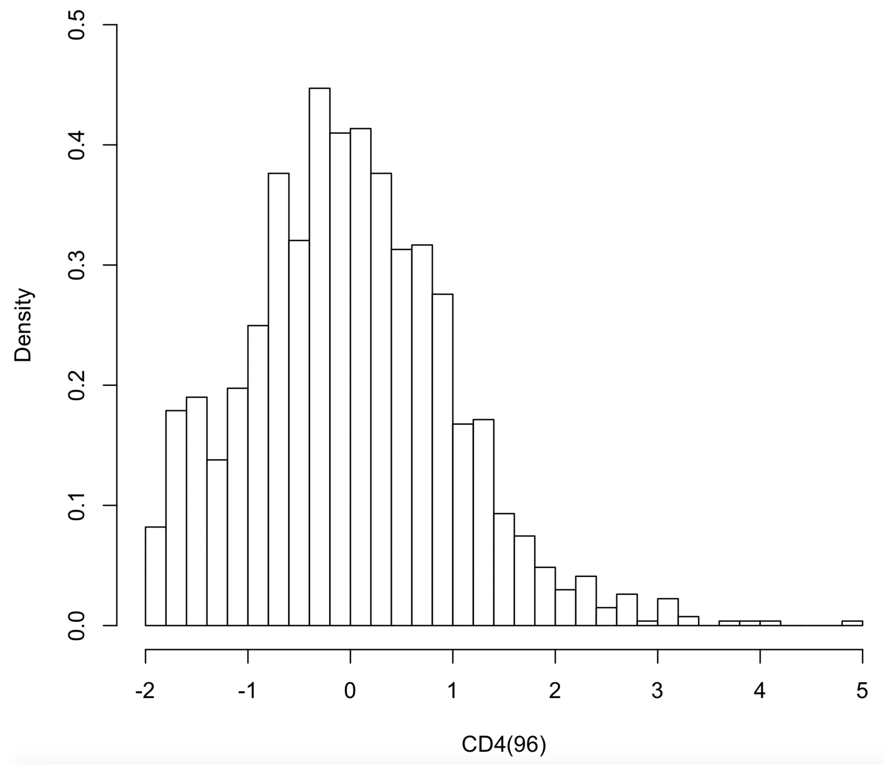
Under the aforementioned data generating mechanism, obtaining an explicit expression for is challenging and requires specifying the working model based on the observed data. In this simulation model, we consider two possible working models: (1) and (2) . Figure 1 and Figure 2 illustrate that the residual distribution of the working model (1) exhibited peakedness, thus violating the normality assumption and indicating model misspecification. In contrast, working model (2) took into account the correct specification of the variance.

Figure 1.
Histogram of the residual distribution for the parameter working model .

Figure 2.
QQ plot of the residual distribution for the parameter working model .
The estimation results of the five types of quantile regression estimates obtained from 1000 random simulations at different quantiles are summarized in Table 3, Table 4 and Table 5. These tables include two types of imputation estimates based on the parameter working models (1) and (2), as well as the corresponding AIPW estimates based on the parameter working models (1) and (2), and the combined estimation equations. The results show that the imputation estimates based on the erroneously specified working model (1) exhibited significant estimation bias. On the other hand, although the working model (2) was also misspecified, it took into account the heteroscedasticity in the conditional distribution of the response variable, thus resulting in smaller estimation bias compared to model (1) and better estimation performance. These findings highlight the sensitivity of imputation methods to misspecified working models. Across the three quantiles, the IPW estimates performed well, thus indicating the robustness of the semiparametric response assumption. Even in the presence of misspecified parameter working models, both of the AIPW estimates had similar median absolute deviations to IPW, which were significantly smaller than the misspecified imputation estimates, thereby demonstrating the robustness of the AIPW estimation. Comparing the two AIPW estimates, it is observed that the estimate based on the correctly specified parameter working model had smaller estimation bias and higher estimation efficiency.
Table 3.
The bias (Bias), standard deviation (SD), and median absolute deviation (MAD) of the five types of quantile regression coefficient estimates at .
Table 4.
The bias (Bias), standard deviation (SD), and median absolute deviation (MAD) of the five types of quantile regression coefficient estimates at .
Table 5.
The bias (Bias), standard deviation (SD), and median absolute deviation (MAD) of the five types of quantile regression coefficient estimates at .
5. Real Data Application
We applied our proposed method to the data of 2139 HIV-infected patients enrolled in the ACTG175 study [27]. The ACTG175 study evaluated the efficacy of monotherapy or combination therapy in HIV-infected patients with CD4 cell counts between 200 and 500 cells/mm3. Following the studies by Davidian et al. [28] and Zhang et al. [29], we categorized all the treatment regimens into two groups. The first group consisted of the standard zidovudine (ZDV) monotherapy arm, while the second group included three newer treatment arms: ZDV and dual nucleoside analogue (ddl), ZDV and zalcitabine (ddC), and ddl monotherapy. The first group comprised 532 subjects, while the second group comprised 1697 subjects. We investigated the effect of the treatment arm (trt, 0 = ZDV monotherapy only) on the quantile of the CD4 cell count () measured at baseline and adjusted for the baseline CD4 cell count () and other baseline covariates, including age, weight, race (0 = Caucasian), gender (0 = female), history of reverse transcriptase inhibitor use (0 = no), and whether the subject discontinued treatment before 96 weeks (offtrt, 0 = no).
Consider fitting a linear quantile regression model as follows:
The dataset used in this study is sourced from the R package “speff2trial”. The study population consists of 1522 Caucasian individuals and 617 non-Caucasian individuals, with 1171 males and 368 females. The average age of the participants is 35 years, with a standard deviation of 8.7 years. Among the participants, 1253 individuals had a history of antiretroviral therapy, and 776 individuals discontinued treatment before the 96th week.
Due to attrition during the study period, approximately 37% of the participants have missing values for the variable . Although complete measurements of other variables related to , such as baseline CD4 and CD8 cell counts and , as well as CD4 and CD8 cell counts at weeks and , were obtained at baseline and follow-up visits, these variables may not fully explain the propensity for participants to drop out. In other words, we cannot assume that the missingness of is random. Therefore, in our analysis, we consider a more comprehensive semiparametric nonrandom missingness mechanism:
where represents the set of variables associated with attrition, and is a function capturing the relationship between these variables and the missingness indicator R.
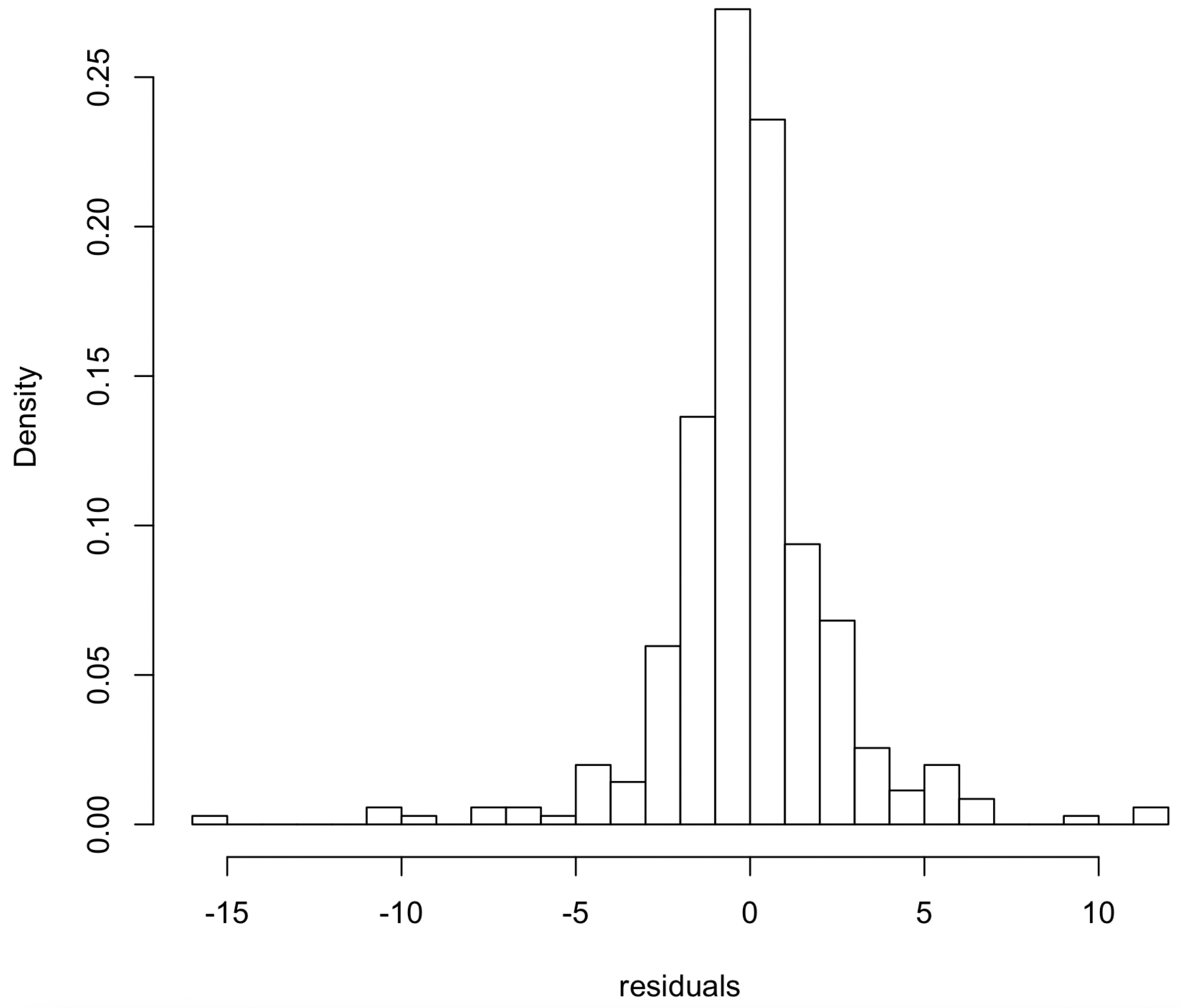
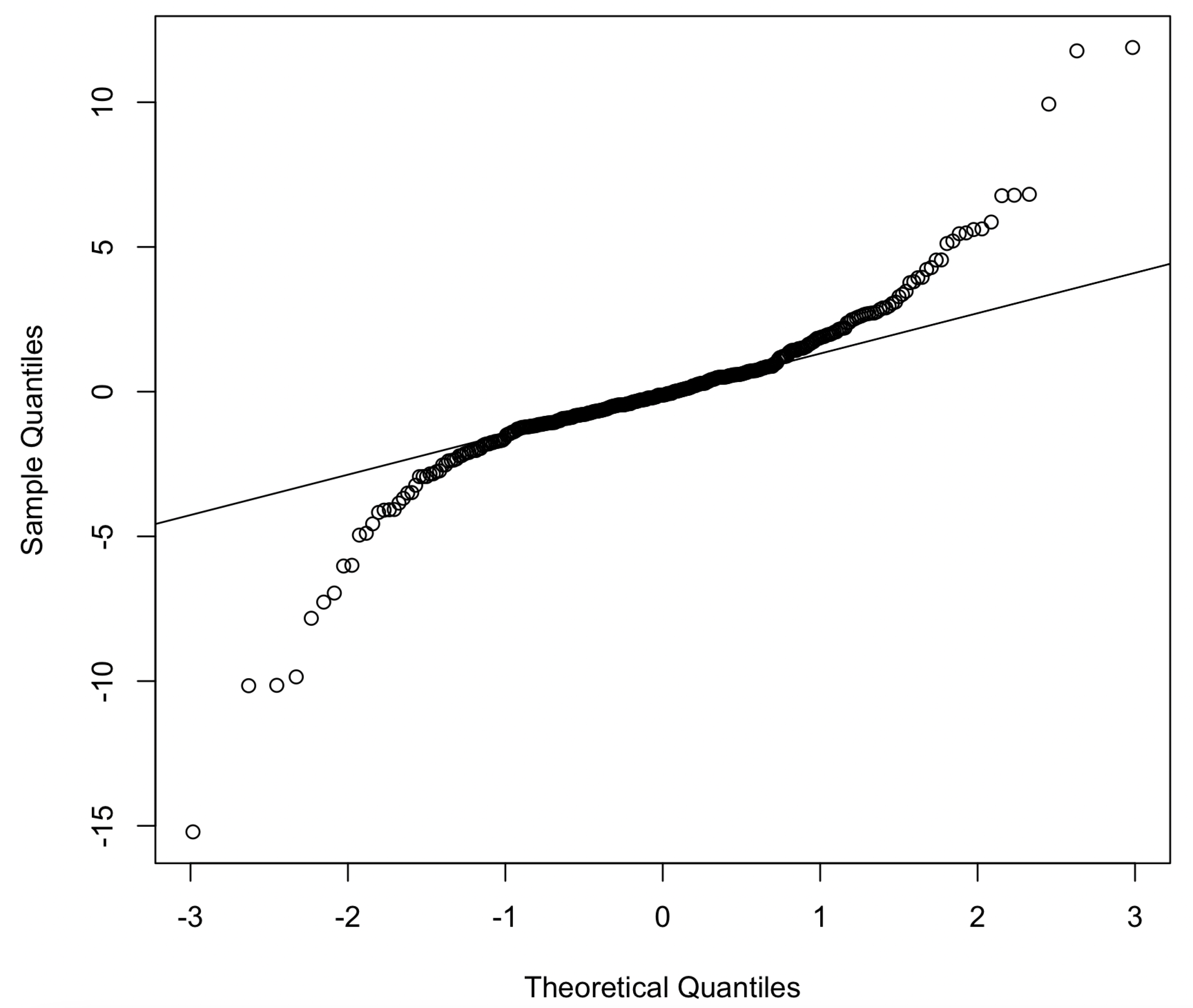
Figure 3 displays the histograms of the observed and its logarithm. From the figure, it can be observed that the conditional distribution of observed is right-skewed. However, the logarithmic transformation did not result in improved symmetry, thus indicating that the normality assumption did not hold. In our analysis, we can assume that follows a truncated normal distribution with left truncation at 0, where its mean is primarily determined by the influence of eight covariates and three auxiliary variables.

Figure 3.
Histogram of complete observed data in ACTG175.
The parameters in the working model are estimated using the truncation regression model in R package "truncreg". The parameter in is estimated using the method of the profile generalized method of moments (GMMs).
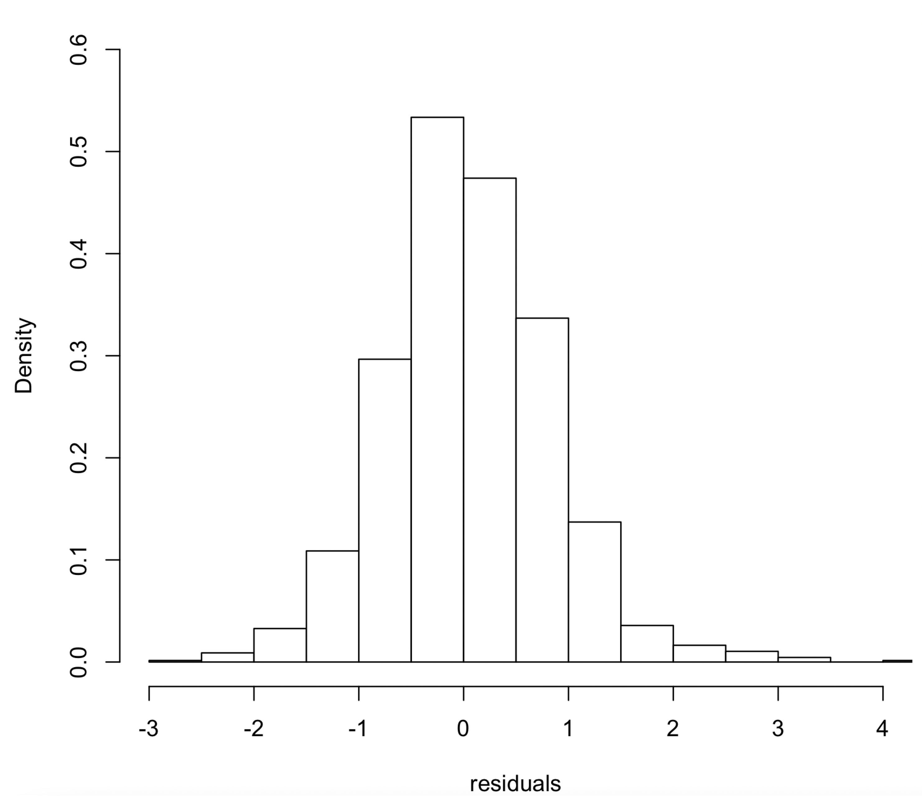
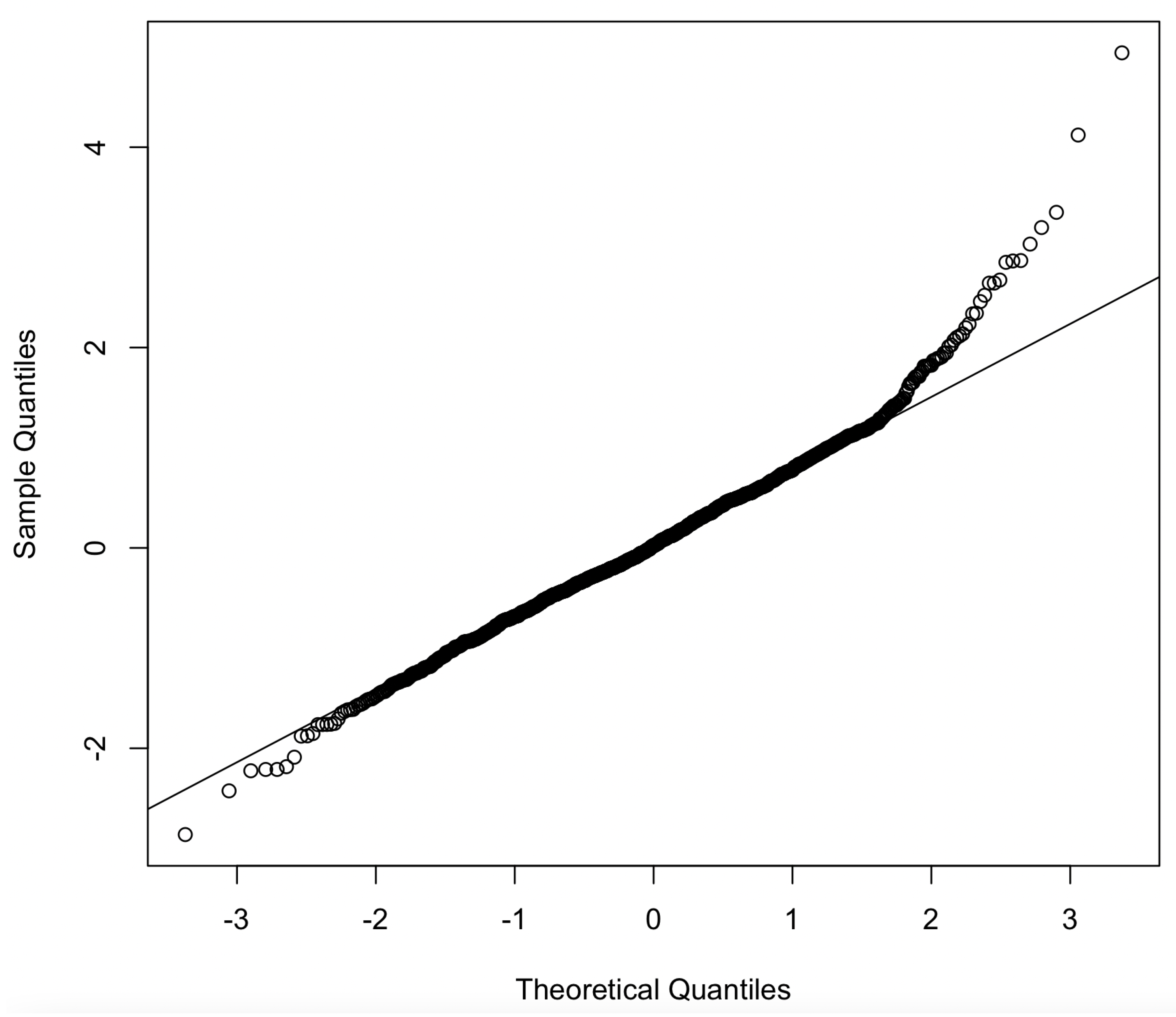
Figure 4 and Figure 5 illustrate the normality properties of the residuals from the truncated regression working model. Visually, the distribution of residuals appears to be symmetric. The calculated sample skewness is 0.05, thus indicating a slight deviation from perfect symmetry. The Q-Q plot reveals that the distribution of residuals has a kurtosis less than 3. Further computation reveals a kurtosis of 2.11, thus indicating that the residual distribution is flatter than a standard normal distribution.
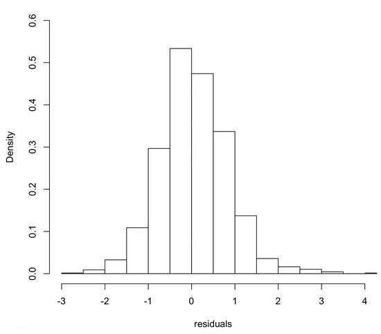
Figure 4.
Histogram of residuals from the parameterized working model.
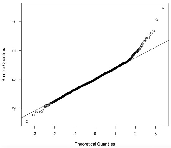
Figure 5.
Q-Q plot of residuals from the parameterized working model.
Table 6 presents the estimates of the quantile regression coefficients and corresponding 95% confidence intervals at the quantile levels. The four estimation methods considered include complete case (CC) estimation, inverse probability weighting (IPW) estimation, multiple imputation (MI) estimation, and augmented inverse probability weighting (AIPW) estimation. The MI estimation is based on averaging over randomly generated imputations. Confidence intervals for the coefficient estimates were obtained using the bootstrap method with resampling iterations.
Table 6.
Analysis results of the ACTG175 dataset.
From Table 6, it can be observed that for the three given quantile levels and four estimation methods, patients receiving the three new combined treatment methods had significantly higher CD4 cell counts at weeks compared to the traditional treatment method. In other words, the new treatment methods had significantly slowed down the progression of AIDS compared to the traditional method. Comparing the four estimation methods, it is evident that the complete case estimation overestimated the performance of the treatment group. The results of the IPW estimation and AIPW estimation were similar and higher than the imputation estimation. When comparing the treatment effects at different quantile levels, both the IPW estimation and imputation estimation reflected a decreasing trend in treatment effect from the 0.25th to the 0.75th quantile. Although the AIPW estimation and complete case estimation did not show a similar trend, the coefficient estimates of the AIPW estimation also indicate a more significant improvement in treatment effect for patients at lower quantiles.
Upon examining the effects of the other covariates, it is found that for all four estimation methods, the baseline CD4 level had a positive impact on the CD4 cell count at weeks, while patients with a history of antiretroviral therapy or early treatment discontinuation exhibited poorer CD4 cell levels at weeks. In comparison to the covariates directly related to the disease progression mentioned above, the effects of age, weight, race, gender, and other covariates on the CD4 cell count at weeks were minimal. The impact directions and significance obtained from different methods were also not consistent. Therefore, although these variables needed to be considered in the modeling process, conclusions regarding their effects should be drawn with caution.
6. Discussion
In this study, we address the bias in quantile regression estimates by constructing imputation and AIPW estimation equations, with both involving the estimation of conditional means under nonrandom missingness. Many existing methods rely on kernel regression to estimate conditional means. However, nonparametric estimation methods may suffer from the curse of dimensionality when the dimension of the covariates is high. Paik and Larsen [19] proposed using importance resampling to obtain Monte Carlo estimates of conditional means, and Song et al. [21] further applied this method to estimation equations. In this study, we extend these methods to quantile regression and overcome the theoretical and computational challenges caused by the nonsmoothness of the checking function in classical quantile regression by employing convolution smoothing.
Common parameter working models are based on linear regression for observed data. Song et al.’s [21] simulation results showed that model misspecification does not lead to estimation bias. However, their simulation study was based on a regression model that satisfied the Gauss–Markov assumption, with missing response variables following a normal distribution with homoscedasticity concerning the covariates. Misspecification was reflected in the estimation of the mean or location variables. However, the advantages of quantile regression are more evident in situations involving skewness, heavy tails, and heteroscedasticity. In this study, our simulation results under heteroscedasticity showed that imputation estimation based on the assumption of a linear regression working model leads to significant estimation bias, while the AIPW estimation equation can mitigate the impact of model misspecification. We also provide theoretical proof of the consistency of AIPW estimation.
Our simulation results demonstrate that, under the ideal scenario of correctly specified parameter working models, the imputation estimator is more efficient than the IPW and AIPW estimators. The AIPW estimator based on the correctly specified model was found to be more efficient than that based on the misspecified model. Therefore, in practical applications, it is crucial to appropriately specify the parameter working model based on the observed data. Fortunately, the effectiveness of the model specification can be assessed using various methods such as Q-Q plots and histograms. For the observed response conditional distributions that do not conform to the linear regression assumption, a Box–Cox transformation can be applied to approximate a normal parameter working model. If such a parameter working model is difficult to obtain, the AIPW estimator proposed in this study can still provide relatively reliable estimates. This is because the proposed response mechanism model is semiparametric and offers certain flexibility. However, the response model constructed in this study does not consider the interaction effects between covariates and the response variable Y or the potential nonlinear effects of the response variable Y on the missingness propensity.
Author Contributions
The first two authors contributed equally to this work. J.G.: Methodology, software, validation, data curation, writing; F.L.: visualization, data curation, review; W.K.H.: writing—review and editing; X.Z.: supervision, validation; K.W.: formal analysis; T.Z.: investigation; L.Y.: resources; M.T.: Conceptualization, project administration, funding acquisition, and the corresponding author. All authors have read and agreed to the published version of the manuscript.
Funding
This research was funded by the Fundamental Research Funds for the Central Universities and the Research Funds of Renmin University of China (22XNL016).
Institutional Review Board Statement
Not applicable.
Informed Consent Statement
Not applicable.
Data Availability Statement
The researchers can download the ACTG175 dataset from the R package “speff2trial”.
Conflicts of Interest
The authors declare no conflict of interest.
Abbreviations
The following abbreviations are used in this manuscript:
| SIR | Sampling Importance Resampling |
| IPW | Inverse Probability Weighting |
| AIPW | Augmented Inverse Probability Weighting |
| EEI | Imputed Estimation Equation |
Appendix A
Appendix A.1. Proof of Lemma 1
Appendix A.2. Proof of Lemma 2
To prove (1), we can perform a simple calculation. We have
Based on the fact that and
we have
Additionally, we have
According to the assumptions, as ,
thus yielding
For , we have
where
Let . By the assumption, we have and . Therefore, as ,
Similarly, let . According to Shao [5], we have and . Thus, as ,
It can be shown that . We have
where
For , and are independent; therefore,
By the assumption, we have . Hence, we can conclude that , which implies
Similarly, we can show that . Consequently,
To establish the asymptotic properties of , we employ Taylor expansions, thus yielding the following:
Consequently, as , we have
where . Furthermore, we obtain
where .
To investigate the asymptotic properties of , we have
Similar to the previous proof, as , we have
where .
To analyze the asymptotic behavior of , we have
According to the analysis, we can conclude that converges to zero in probability, i.e., .
To establish the asymptotic properties of , we have
where .
According to the Slutzky theorem, we have
where . Similarly to the previous proof, it can be shown that
which implies that, as ,
where .
To prove (2), we first establish the asymptotic property of . By the law of large numbers and the fact that and , we have
As , under the assumption, we have
Therefore,
Similarly, for , we have
As , under the assumption, we have
Therefore, we have
Next, we prove (3). Note that, for , we have
By the law of large numbers, as , we have .
Finally, we demonstrate (4). From
it can be easily shown that, for , .
Proof of Theorem 1.
By applying the Lagrange multiplier method, we obtain the empirical log-likelihood ratio function with respect to the parameter vector :
where is the solution to the following equation:
In other words, simultaneously satisfies the following two equations:
Note that , and . Under the assumption conditions, according to Lemma A.1 in Newey and Smith [30] and Theorem 1(a) in Leng and Tang Leng [31], it can be shown that is a consistent estimator of . By Taylor expanding and around , we have
where .
The above equations can be rewritten as follows:
Based on the results of Lemma 2, we have
Therefore, for and as , we have
□
Proof of Theorem 2.
First, we note that . Let , where and . We have
By multiplying both sides of the equation by , we obtain
Thus, we can conclude that
Based on Lemma 2, we have
Consequently, it follows that . Furthermore, we can observe that
By expanding the function , we obtain
where . From the fact that , it follows that .
Note that
Therefore,
where .
By expanding around using a Taylor series, we obtain
Similarly,
Therefore, we obtain
By combining the previous results, we can express
Here, . Thus,
Based on the results (1) and (2) of Lemma 2, it can be easily demonstrated that, as n tends to infinity, the asymptotic distribution of follows a linear combination of independent chi-squared random variables:
where represents the eigenvalues of . Here, denote q independent standard chi-squared distributed random vectors. This completes the proof of the theorem. □
References
- Robins, J.M.; Ritov, Y. Toward a curse of dimensionality appropriate (CODA) asymptotic theory for semi–parametric models. Stat. Med. 1997, 16, 285–319. [Google Scholar] [CrossRef]
- Wang, S.; Shao, J.; Kim, J.K. An instrumental variable approach for identification and estimation with nonignorable nonresponse. Stat. Sin. 2014, 24, 1097–1116. [Google Scholar] [CrossRef]
- Kenward, M.G. Selection models for repeated measurements with non–random dropout: An illustration of sensitivity. Stat. Med. 1998, 17, 2723–2732. [Google Scholar] [CrossRef]
- Kim, J.K.; Yu, C.L. A semiparametric estimation of mean functionals with nonignorable missing data. J. Am. Stat. Assoc. 2011, 106, 157–165. [Google Scholar] [CrossRef]
- Shao, J.; Wang, L. Semiparametric inverse propensity weighting for nonignorable missing data. Biometrika 2016, 103, 175–187. [Google Scholar] [CrossRef]
- Kim, J.K.; Shao, J. Statistical Methods for Handling Incomplete Data; CRC Press: New York, NY, USA, 2022. [Google Scholar]
- Koenker, R.; Bassett, G. Regression quantiles. Econometrica 1978, 46, 33–50. [Google Scholar] [CrossRef]
- Koenker, R.; Bassett, G. Tests of linear hypotheses and L1 estimation. Econometrica 1982, 50, 1577–1583. [Google Scholar] [CrossRef]
- Horowitz, J.L. Bootstrap methods for median regression models. Econometrica 1998, 66, 1327–1351. [Google Scholar] [CrossRef]
- Whang, Y.J. Bootstrap methods for median regression models. Econ. Theory 2006, 22, 173–205. [Google Scholar]
- Luo, S.H.; Mei, C.L.; Zhang, C.Y. Smoothed empirical likelihood for quantile regression models with response data missing at random. Adv. Stat. Anal. 2017, 101, 95–116. [Google Scholar] [CrossRef]
- Zhang, T.; Wang, L. Smoothed empirical likelihood inference and variable selection for quantile regression with nonignorable missing response. Comput. Stat. Data. Anal. 2020, 144, 106888. [Google Scholar] [CrossRef]
- Niu, C.; Guo, X.; Xu, W.; Zhu, L. Empirical likelihood inference in linear regression with nonignorable missing response. Comput. Stat. Data. Anal. 2014, 79, 91–112. [Google Scholar] [CrossRef]
- Bindele, H.F.; Zhao, Y.C. Rank-based estimating equation with non-ignorable missing responses via empirical likelihood. Stat. Sin. 2018, 28, 1787–1820. [Google Scholar] [CrossRef]
- Chen, X.R.; Wan, A.T.K.; Zhou, Y. Efficient quantile regression analysis with missing observations. J. Am. Stat. Assoc. 2015, 110, 723–741. [Google Scholar] [CrossRef]
- Tang, N.S.; Zhao, P.Y.; Zhu, H.T. Efficient quantile regression analysis with missing observations. Stat. Sin. 2014, 24, 723–747. [Google Scholar] [PubMed]
- Kim, J.K. Parametric fractional imputation for missing data analysis. Biometrika 2011, 98, 119–132. [Google Scholar] [CrossRef]
- Riddles, M.K.; Kim, J.K.; Im, J. A propensity-score-adjustment method for nonignorable nonresponse. J. Surv. Stat. Methodol. 2016, 4, 215–245. [Google Scholar] [CrossRef]
- Paik, M.; Larsen, M.D. Handling nonignorable nonresponse with respondent modeling and the SIR algorithm. J. Stat. Plan. Inference 2014, 145, 179–189. [Google Scholar] [CrossRef]
- Wang, X.L.; Song, Y.Q.; Lin, L. Handling estimating equation with nonignorably missing data based on SIR algorithm. J. Comput. Appl. Math. 2017, 326, 62–70. [Google Scholar] [CrossRef]
- Song, Y.Q.; Zhu, Y.J.; Wang, X.L.; Lin, L. Robust inference for estimating equations with nonignorably missing data based on SIR algorithm. J. Stat. Comput. Simul. 2019, 89, 3196–3212. [Google Scholar] [CrossRef]
- Newey, W.K.; McFadden, D. Large sample estimation and hypothesis testing. In Handbook of Econometrics; Engle, R.F., McFadden, D., Eds.; Elsevier: Amsterdam, The Netherlands, 1994; pp. 2111–2245. [Google Scholar]
- Van der Vaart, A.W. Semiparametric statistics. In Lectures on Probability Theory and Statistics (Saint-Flour, 1999); Bernard, P., Ed.; Springer: Berlin, Germany, 2002; pp. 331–457. [Google Scholar]
- Morikawa, K.; Kim, J.K.; Kano, Y. Semiparametric maximum likelihood estimation with data missing not at random. Can. J. Stat. 2017, 45, 393–409. [Google Scholar] [CrossRef]
- Morikawa, K.; Kim, J.K. Semiparametric optimal estimation with nonignorable nonresponse data. Ann. Stat. 2021, 49, 2991–3014. [Google Scholar] [CrossRef]
- Zhao, P.; Wang, L.; Shao, J. Empirical likelihood and Wilks phenomenon for data with nonignorable missing values. Scan. J. Stat. 2019, 46, 1003–1024. [Google Scholar] [CrossRef]
- Hammer, S.M.; Katzenstein, D.A.; Hughes, M.D.; Gundacker, H.; Schooley, R.T.; Haubrich, R.H.; Henry, W.K.; Lederman, M.M.; Phair, J.P.; Niu, M.; et al. A trial comparing nucleoside monotherapy with combination therapy in HIV-infected adults with CD4 cell counts from 200 to 500 per cubic millimeter. N. Engl. J. Med. 1996, 335, 1081–1090. [Google Scholar] [CrossRef] [PubMed]
- Davidian, M.; Tsiatis, A.A.; Leon, S. Semiparametric estimation of treatment effect in a pretest–posttest study with missing data. Stat. Sci. 2005, 20, 261–301. [Google Scholar] [CrossRef] [PubMed]
- Zhang, M.; Tsiatis, A.A.; Davidian, M. Improving efficiency of inferences in randomized clinical trials using auxiliary covariates. Biometrics 2008, 64, 707–715. [Google Scholar] [CrossRef]
- Newey, W.K.; Smith, R.J. Higher order properties of GMM and generalized empirical likelihood estimators. Econometrica 2004, 72, 219–255. [Google Scholar] [CrossRef]
- Leng, C.L.; Tang, C.Y. Penalized empirical likelihood and growing dimensional general estimating equations. Biometrika 2012, 99, 703–716. [Google Scholar] [CrossRef]
Disclaimer/Publisher’s Note: The statements, opinions and data contained in all publications are solely those of the individual author(s) and contributor(s) and not of MDPI and/or the editor(s). MDPI and/or the editor(s) disclaim responsibility for any injury to people or property resulting from any ideas, methods, instructions or products referred to in the content. |
© 2023 by the authors. Licensee MDPI, Basel, Switzerland. This article is an open access article distributed under the terms and conditions of the Creative Commons Attribution (CC BY) license (https://creativecommons.org/licenses/by/4.0/).