Abstract
As a crucial component of enterprise marketing strategy, commodity pricing and replenishment strategies often play a pivotal role in determining the profit of retailers. In pursuit of profit maximization, this work delved into the realm of fresh food supermarket commodity pricing and replenishment strategies. We classified commodities into six distinct categories and proceeded to examine the relationship between the total quantity sold in these categories and cost-plus pricing through Pearson correlation analysis. Furthermore, a Seasonal ARIMA model was established for the prediction of replenishment quantities and pricing strategies for each of the categories over a seven-day period. To ensure precise data, we extended our forecasting to individual products for a single day, employing 0–1 integer programming. To align the inquiry with real-world scenarios, we took into account various factors, including refunds, waste, discounts, and the requirement that individual products fall within specific selling ranges. The results show that the profit will be maximized when the replenishment of chili is 39.874 kg and the replenishment of edible mushrooms is 43.257 kg in the future week. We assume that the residual of the model is white noise. By testing the white noise of the model, the analysis of the residual Q statistic results shows that it is not significant in level, which can prove that the model meets the requirements and the obtained results are reliable. This research provides valuable insights into the realm of commodity pricing and replenishment strategy, offering practical guidance for implementation.
Keywords:
commodity pricing; replenishment strategy; cost-plus pricing; seasonal ARIMA model; Pearson correlation analysis MSC:
91G10; 90C90; 90C30
1. Introduction
With the fast development of the social economy and urbanization, the standard of living for people continues to improve. To meet the increasing demand for fresh produce, a growing number of fresh food supermarkets are emerging in urban and rural areas. Fresh foods primarily encompass fruits, vegetables, aquatic products, meat, and various food items [1]. Due to their short shelf life and susceptibility to spoilage, they are commonly referred to as perishable goods and must be marketed within a restricted timeframe. For supermarket proprietors, maximizing profit remains a top priority. The perishable nature of general fresh goods results in their rapid deterioration over time, impacting profitability significantly. Our model is designed with an objective function aiming to maximize profit by determining optimal pricing and replenishment strategies, thereby enhancing overall profitability. Conversely, consumers prioritize fresh foods for their health-conscious choices, leading their purchasing decisions to heavily rely on product freshness. Our proposed replenishment strategy serves as a timely reminder for supermarkets to restock their shelves, ensuring a certain level of product freshness. Furthermore, given the diverse range of vegetable varieties available in supermarkets, coupled with varying origins, purchasing transactions for these vegetables typically occur between 3:00 and 4:00 in the morning. Consequently, businesses are required to make daily replenishment decisions for each vegetable category without precise information regarding specific products and purchase prices. Consequently, the importance of devising well-crafted commodity pricing and replenishment strategies cannot be overstated.
In recent years, there has been a growing body of research dedicated to commodity pricing. Most research uses mathematical models to solve problems. Initially, Emanuele et al. [2] conducted research on vanilla-option pricing by using the Ornstein–Uhlenbeck process and the two-factor mean-reverting process. The introduction of these two models expanded the scope of the research beyond the geometric Brownian model. Subsequently, Guo [3] proposed a model that combines CNN (Convolutional Neural Network) with an attention mechanism to encode image features and select commodity image features. This fusion of machine learning and models improved the approach to handling commodity pricing. Afterward, Chen et al. [4] conducted a study on the pricing of Brent crude oil using a three-factor model with random volatility. In comparison to the previous two-factor model for commodity futures pricing, the three-factor model demonstrates a better fit for contracts with longer maturities. Meanwhile, Crosby and Frau [5] introduced a novel term-structure model for commodity futures prices, building upon previous research by incorporating multiple jump processes. Nevertheless, it is worth noting that the majority of these studies predominantly focus on stable commodities that do not decay over time, leaving the realm of perishable goods unexplored. In the context of perishable goods, Liang et al. [6] introduced a bi-objective, multi-period vehicle routing model for perishable goods delivery. They developed a combined variable neighborhood search (VNS) and simulated annealing (SA) metaheuristic algorithm based on the ε-constraint method, incorporating transportation costs and customer satisfaction. Reza et al. [7] optimized the sales level of perishable goods in a two-echelon green supply chain, concurrently considering the optimization of two objective functions. However, these studies often delve into the intricacies of supply chain management and inventory control, overlooking commodity pricing and replenishment decision strategies. Zhao et al. [8] investigated the adoption decision of a block chain-based traceability system in the dual-channel perishable goods market under various pricing policies, employing a game-theoretical model that accounts for both perishable goods and commodity pricing. In China, Zhao and Wang [9] proposed the basic pricing model for group-buying fresh electricity suppliers under a cooperation model between merchants and group-buying platforms. Zhang and Mo [10] introduced ordering and pricing strategies for perishable inventory based on the Weibull function and price discounts, but did not consider the situation of sales returns. Guo [11] incorporated sales returns into dynamic models, although seasonal factors were not considered. Across the seas, Chun [12] explored price-making rules for perishable foods in single-period and multi-period scenarios, considering the optimal order quantity that maximizes the seller’s total expected profit. Elmaghraby’s team [13] conducted a comprehensive investigation to determine the number of discount periods that could maximize supermarket profits. Aviv and Pazgal [14] assumed a single discount period followed by reduced prices, acknowledging that this assumption might not always hold, as buyers may still negotiate for lower prices. Maihami and Nakhai [15] introduced a unique approach by formulating a function to determine optimal selling prices and replenishment schedules, even accommodating shortages and backlogs. Surprisingly, their findings suggested that a single discount period is the most effective strategy.
Current studies predominantly focus on perishable products from the supply chain and inventory perspectives, neglecting in-depth analysis of pricing and replenishment strategies. Moreover, prevailing pricing research tends to establish profit maximization models for a single stage, overlooking the influence of changes in freshness on consumer behavior, which fails to reflect the multifactorial nature of real-world scenarios. Our approach, employing the cost-plus pricing method in this study, considers the influence of fresh goods’ freshness on pricing. This method accounts for practical aspects, such as discounted sales due to transport damage or product phase changes. Additionally, integrating seasonal effects into the commonly used ARIMA model enhances its applicability and aligns it more closely with real-world dynamics, signifying increased practical significance. The current research on replenishment strategies often fails to consider comprehensive factors, largely ignoring issues of stock shortages and product freshness. This oversight poses practical challenges in its application. By adopting the 0–1 planning model, our study overcomes these limitations. This model excels in scenarios involving numerous complex interrelated factors, effectively addressing replenishment issues. Finally, our research explores both pricing and replenishment strategies in fresh supermarkets, considering seasonality, shortages, returns, discount sales, and other factors. This comprehensive approach enhances existing models and provides valuable insights for decision-making in real supermarket scenarios. After considering these factors, our paper examines 251 common single vegetables found in fresh food supermarkets, categorizing them into six distinct groups for in-depth analysis. Then, we further gathered a database from the fresh food supermarket, encompassing details on individual products and categories, comprehensive sales data, wholesale prices, and the attrition rates of goods. In this work, we chose vegetable products as an example. Although the storage requirements and shelf life of fruits may differ slightly, we have adapted our models to ensure wider applicability to fruit products. The varying storage conditions and shelf life of fruits available in supermarkets affect their freshness differently. Our model accounts for these freshness differences by reflecting them in attrition rates. Consequently, these attrition rates within the cost-plus pricing model influence the total variable cost, subsequently impacting the pricing strategy applied to fruits. Therefore, our model is also applicable to fruit products. To address the challenge, we employ a combination of approaches, including cost-plus pricing, Seasonal ARIMA modeling, Pearson correlation analysis, linear regression modeling, and 0–1 integer programming. From a data-driven perspective, the application of statistical methods and machine learning techniques represents a distinctive advantage and innovation in our research.
The subsequent sections of this paper are organized as follows: Section 2 introduces the preparation for modeling, encompassing assumptions and data pre-processing. Section 3 outlines the development of detailed models for forecasting replenishment volumes and pricing strategies. In Section 4, the analyses of the model’s results are presented. Section 5 offers discussions and suggestions based on the findings. Lastly, Section 6 summarizes the entirety of this work. This paper aims to provide a comprehensive exploration of commodity pricing and replenishment strategies, offering valuable insights and guidance for the management of retailers.
2. Preparation for Modeling
2.1. Modeling Assumptions and Data Pre-Processing Methods
Three primary assumptions are considered during the modeling:
Assumption 1.
Fresh foods are assumed not to incur significant damage due to highly unusual situations, e.g., truck accidents or negligence of employees.
Assumption 2.
The sales dynamics in this scenario adhere to conventional market laws.
Assumption 3.
The supermarket is assumed to replenish its inventory sufficiently early to prevent shortages of food products for customers.
To facilitate modeling and analysis, we conducted several preprocessing steps on the data:
- Categorization: All single products were grouped into six distinct categories: floral leaf, cauliflower, aquatic rhizome, solanaceous, chili, and edible mushroom.
- Missing Data Handling: Due to discontinuities in the recorded data, we employed window mean or regression methods to fill in the gaps in the data time points.
- Outlier Identification: We identified outlier data and addressed it using techniques such as moving averages and direct deletion.
- Data Standardization: The data were standardized, scaling it to a zero-mean homoscedastic interval to ensure dimensionless features across multiple data points.
2.2. Relationship between Cost-Plus Pricing and Other Influential Factors
2.2.1. Cost-Plus Pricing
The cost-plus pricing is based on the unit cost of the product in the sales process, coupled with the expected profit, to determine the price [16]. The price difference between the original price and the discount price will be considered in our model system, and this difference impacts the price of food when it is sold the next day. Traditional enterprises usually determine their commodities’ price by the market price because it is easy to choose the lowest cost price. However, problems arise when merchants do not have sufficient communication with the product supplier. This can make cost-price management challenging, and if there is an increase in demand, there may be inventory shortages. Except for the cost price and the cost of foods’ damage due to freshness, cost-plus pricing ensures a specific profit, which helps stabilize commodity prices over a period of time. We use this method to simulate commodity pricing because it is more practical and easier to understand. The detailed calculation method for cost-plus pricing is as follows:
- (1)
- Total fixed cost W is calculated as the product of unit selling price a and the quantity of sale d, while the total variable cost R is determined by multiplying the attrition rate s by the quantity of sale d:W = a × d, R = s × d
- (2)
- The unit cost C is obtained by summing the total fixed cost W and the total variable cost R:C = W + R
- (3)
- The markup rate Q is the quotient of unit cost and sales quantity d multiplied by the difference between selling price and purchase price divided by the sum of the quotient and 1 of the purchase price:
- (4)
- Cost-plus pricing P is:P = C × (1 + Q)
- (5)
- Substituting Equations (2) and (3) into Equation (4), we obtain the final Cost-plus pricing P as:
2.2.2. Pearson Correlation Analysis
In studies involving two continuous variables, typically referred to as x-values and y-values, the presence of a linear relationship between these two variables can be assessed using the Pearson correlation coefficient [17].
In order to study the relationship between total sales quantity and cost-plus pricing, this section introduces Pearson correlation analysis. In this situation, the Pearson correlation coefficient can be calculated as the product of the covariance of two variables and their respective standard deviations. If two variables both tend to increase or decrease together, the Pearson correlation coefficient will be close to −1 or 1. In the absence of a linear relationship, the Pearson correlation coefficient will approach 0. Consequently, we can explore the relationship between the two indices. The correlation formulas are as follows:
- Covariance of samples:
- Standard deviation of samples:
- Pearson correlation coefficient of samples:
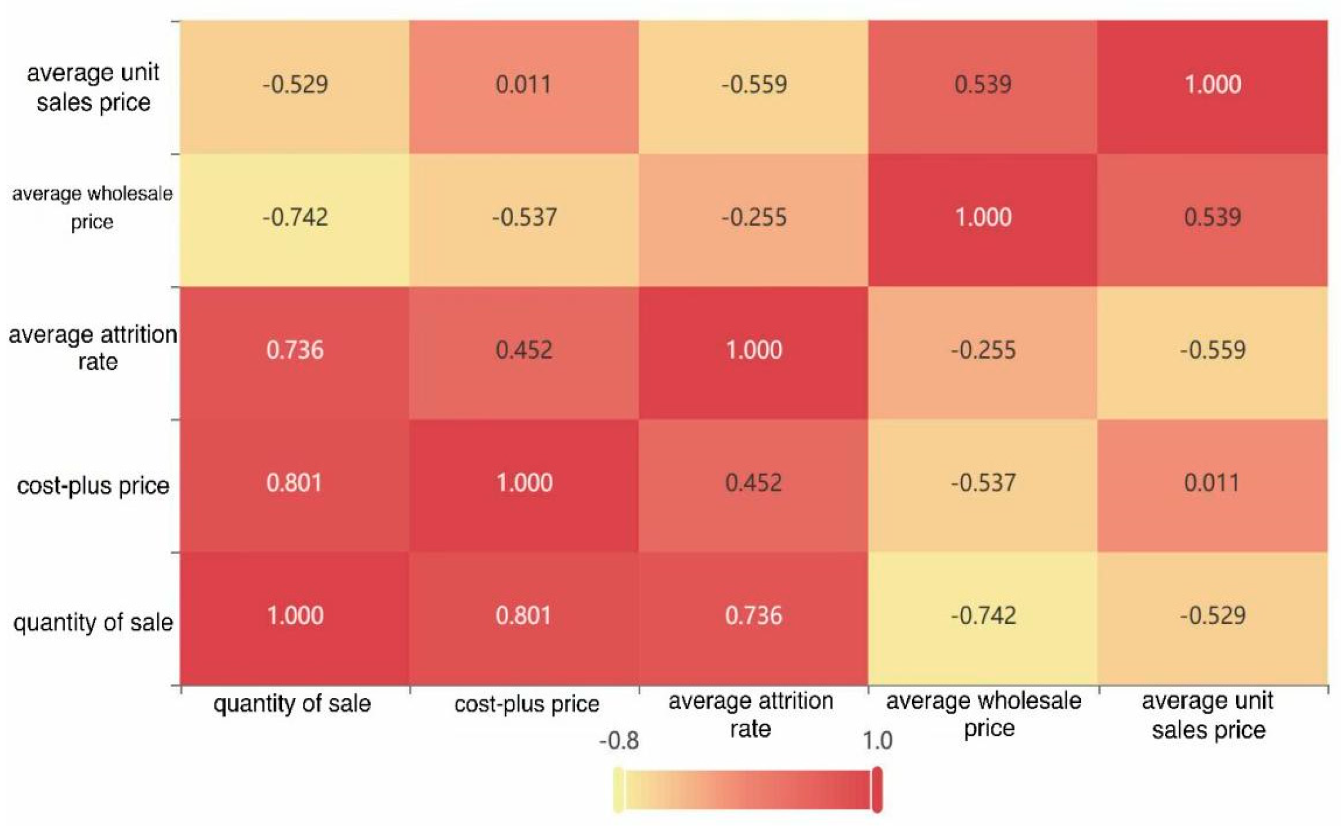
Figure 1 shows the thermodynamic chart of the correlation coefficient. It can be seen that the quantity of sales for each product category has the strongest correlation with cost-plus pricing, has a strong correlation with the average attrition rate, but has a negative correlation with the average wholesale price and the average unit sales price. The cost-plus pricing has the strongest correlation with the quantity of sales for each product category, a weak correlation with the average attrition rate and the average unit sales price, and a negative correlation with the average wholesale price.
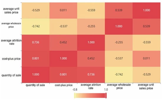
Figure 1.
The thermodynamic chart of the correlation coefficient.
3. Establishment of a Model
3.1. Prediction of the Replenishment Quantity in Categories
The Auto Regression Integrated Moving Average (ARIMA) model is widely used for modeling and predicting non-seasonal time series data [18]. The Seasonal ARIMA model, an extension of the ARIMA model, incorporates seasonal factors, allowing it to predict time series data with seasonal variations. Since the time series data for fresh foods exhibits both seasonal and trend variations and customer preferences and available commodities change with the seasons, the Seasonal ARIMA model is well-suited for forecasting replenishment decisions in fresh supermarkets.
To predict the replenishment quantity for a seven-day period, this paper employs the seasonal ARIMA model, which has been widely used as a seasonal time series model for the past three decades [19]. A seasonal ARIMA model typically comprises three components: the autoregressive (AR) component, the differencing (I) component, and the moving average (MA) component. The AR component considers the impact of past time point values on the current value, reflecting real-world scenarios where past sales differences affect product inventory and subsequently influence replenishment quantities. The differencing component helps eliminate time series non-stationarity, simplifying the prediction process. The moving average component takes into account the influence of errors at past time points on the current value, leading to more accurate predictions. In the Seasonal ARIMA model, all three components incorporate seasonality. For each product category, this paper establishes a seasonal ARIMA model, and the detailed steps and results are presented below:
- (1)
- At first, we calculate the total sales volume of each category from 1 July to 7 July in 2020, 2021, and 2022 and draw the sales timing charts for them. Then, we decompose the time series into trend data, seasonal data, and random data to preliminarily judge the seasonal effect of the data.
- (2)
- To prove the stationarity of time series, we did an ADF test on six categories. If p < 0.05, the series is stationary. If the original time series does not satisfy stationarity, it will be differentiated and seasonally differentiated until the series satisfies stationarity.
- (3)
- According to the results of the ADF test, the optimal difference can be found. Then, we established the ACF (auto-correlation function), which describes the linear correlation between time series observations and their past observations. The calculation formula is as follows:Here, k represents the number of lag periods and represents the sequence value. To conduct a more comprehensive analysis, we eliminated interference and examined the Partial Autocorrelation Function (PACF) of the differenced data. The method for analyzing key parameters and the legend entry are identical to those used for the ACF. To reflect the degree of correlation between variables, we draw an autocorrelation chart of final differential data and a partial autocorrelation chart of final differential data. And in order to make the predicted values more visible, we also draw the time series prediction chart.
- (4)
- Solving the models, we obtain the replenishment quantity of six categories in seven days, which can make the income of the supermarket maximal.
3.2. Prediction of Pricing Strategy in Categories
In this section, we utilize linear regression [20] to forecast the pricing strategy for the next seven days. Linear regression is popular for various applications due to its simplicity and the ability to model regression functions as linear combinations of predictors [21]. Here, we constructed a linear regression model using sales data from 1 to 7 July 2022, and subsequently analyzed the results from various perspectives.
First, an F-test was performed to determine whether there was a significant linear relationship. By analyzing the F value, it is determined whether it can significantly reject the null hypothesis that the population regression coefficient is 0 (p < 0.05). If it is significant, it indicates that there is a linear relationship. Then, the VIF value represents the severity of multicollinearity and is used to test whether the model presents collinearity, that is, whether there is a highly correlated relationship between explanatory variables (VIF should be less than 10 or 5, strictly 5). If VIF appears inf, it indicates that the VIF value is infinite. It is recommended to check collinearity or use ridge regression. So VIF values were analyzed to determine whether the model presented collinearity. Afterwards, according to the analysis, we make sure to obtain the model formula. Finally, in order to observe the function expression more directly, we draw the fitting effect diagram, which shows the original data diagram and the predicted value of this model. By substituting the daily replenishment data of the six categories of vegetables in the next week into the model formula, the pricing strategy for the next week can be obtained.
3.3. Prediction of Pricing and Replenishment Strategies for a Single Product
Integer programming models have gained significant traction in addressing various management and problem-solving scenarios [22]. Particularly, 0–1 integer programming, focused on optimizing objective functions with binary variable constraints, is employed in this study to maximize supermarket profit. Its ability for variable selection and feature engineering makes it well-suited for complex real-world problems, enhancing interpretability and practicality [23]. Using 0–1 integer programming, we predict pricing and replenishment strategies for individual products, contributing to improved decision-making.
To facilitate modeling, we preprocessed the data. Initially, we receive the sales items for the period of 24 to 30 June 2023, identifying 49 items available for sale during this timeframe. Ensuring compliance with the minimum order quantity of 2.5 kg for each product, we filtered out 10 items with orders below this threshold, resulting in a total of 39 items available for sale. Furthermore, we factored in commercial excess capacity and market demand constraints by calculating the sum of individual vegetables in commercial excess for each day from 24 to 30 June, determining maximum and minimum values. Similarly, akin to our approach for establishing the pricing strategy for each product category in the following week, we employed a linear regression model to analyze the correlation between the sales volume of each vegetable item and cost-plus pricing for the period of 24–30 June 2023, deriving a relationship formula as follows:
The total profit available to the supermarket is calculated by multiplying the net profit for each successfully sold individual product by its corresponding sales volume and then summing these values. In order to maximize the supermarket’s profit, the objective function is formulated as follows:
where is a 0–1 parameter. When its value is 1, it means that the sales item is sold on the day, and 0 means that it is not sold on the day. It can be summarized as:
There are some constraint conditions in the model:
- Single product display quantity constraint: the replenishment quantity of each vegetable single product should meet the conditions of the minimum display quantity of 2.5 kg:
- Restriction on the total number of salable items: In the development of the replenishment plan for the single item, the total number of salable items should be controlled between 27 and 33:
- Supermarket capacity constraint: Due to the limited sales space of supermarket products, the replenishment volume of single items on July 1 should be less than the maximum sales volume of single items (vegetables) in supermarkets from 24 to 30 June:
- Equation constraint: Sales volume and commodity cost plus pricing meet:
Based on the above analysis, we established the optimization model as follows:
- Objective function:
- Constraint conditions:
4. Results and Analysis
4.1. Prediction of the Replenishment Quantity in Categories
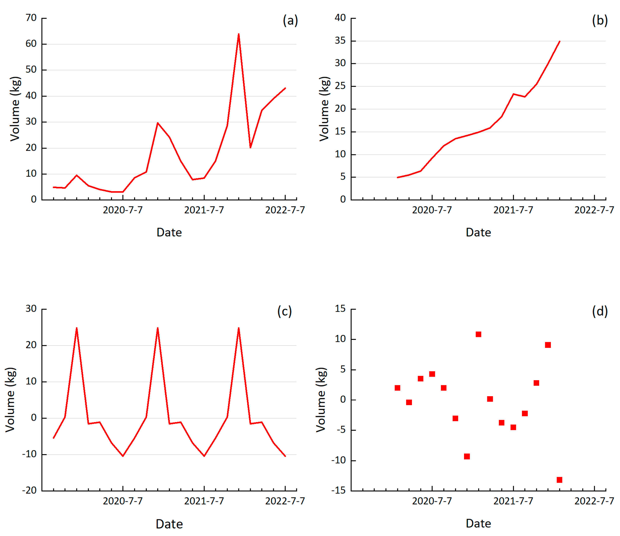
We draw the primary sequence, trend sequence, seasonal sequence, and random sequence charts of different categories. There are six categories of floral leaf category, cauliflower category, aquatic rhizome category, solanaceous category, chili category, and edible mushroom category in the given data. It is too tedious to show them all; here, the aquatic rhizome category is taken as an example to illustrate, as shown in Figure 2.
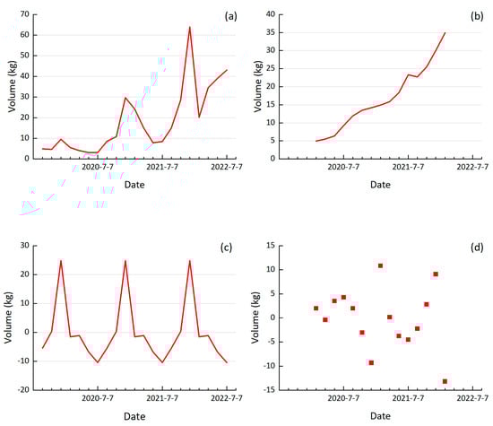
Figure 2.
Sequence charts for the aquatic rhizome category. (a) Primary sequence chart; (b) Trend sequence chart; (c) Seasonal sequence chart; (d) Random sequence chart.
For the ADF test of six categories, we take aquatic rhizomes, for example, and the detailed data are as follows:
The above table includes variables, difference order, t test result, AIC value, etc., which are used to test whether the time series data are stationary. Here, AIC is a standard for measuring the good fit of a statistical model. The model necessitates that the series be stationary time series data. By analyzing the p value, we can determine whether it can reject the null hypothesis of sequence instability significantly. If it is significant (p < 0.05), it means that the null hypothesis is rejected and the series is a stationary time series; otherwise, it means that the series is an unstable time series. From the table, we can see that when the series makes a 1st order difference-1st order seasonal difference, the value of p is 0.00, which is smaller than 0.05, which means the optimal difference is a 1st order difference-1st order seasonal difference. The critical values of 1%, 5%, and 10% represent statistical thresholds for different degrees of rejecting the null hypothesis. ADF test results that are simultaneously less than 1%, 5%, and 10% indicate a robust rejection of the hypothesis.
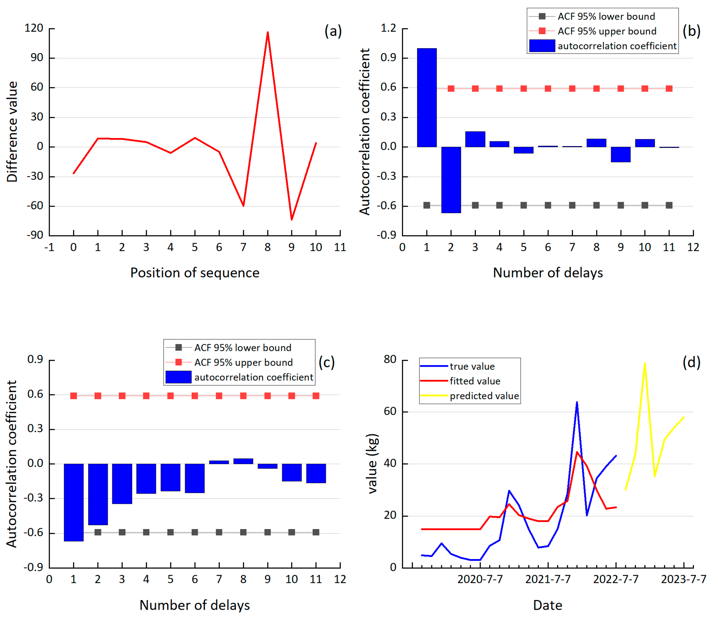
According to Table 1, it can be found that the optimal difference is a 1st order difference-1st order seasonal difference. Hence, the data of 1st order difference-1st order seasonal difference was chosen for analysis as shown in Figure 3a. The ACF results of the final difference data are shown in Figure 3b, which includes coefficients and upper and lower confidence limits, where the blue column represents the coefficient of auto-correlation, the black line represents the 95% lower bound of ACF, and the red line represents the 95% upper bound of ACF. The horizontal axis represents the number of delays, and the vertical axis represents the auto-correlation coefficient. It can be seen from the figure that the autocorrelation coefficient is zero after the delay of order 2, so it can be concluded that the truncation is order 2. This indicates that the seasonal effect has been completely eliminated after order 2 in this difference. The partial autocorrelation chart of the final differential data are illustrated in Figure 3c. It is obviously that the seasonal effect has been completely eliminated after order 1 in this difference. For clarity and a dynamic presentation of the results, we created the time series in Figure 3d. In this figure, the blue, red, and yellow lines represent the actual data, model-fitted values, and model-predicted values, respectively.

Table 1.
ADF test list of the aquatic rhizomes.
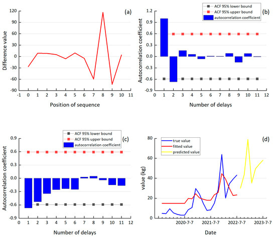
Figure 3.
Analysis and prediction of aquatic rhizomes: (a) optimal difference sequence chart; (b) autocorrelation chart of final differential data; (c) partial autocorrelation chart of final differential data; (d) time series prediction chart.
Taking 1 to 7 July 2023, as an example, the total daily replenishment of six categories of commodities in the next week is predicted as shown in Table 2. From the table, we can obtain a detailed replenishment quantity of six categories in seven days, which can make the income of the supermarket maximal.
Table 2.
Next week’s replenishment forecast table (kg).
4.2. Prediction of Pricing Strategy in Categories
To maintain brevity, we present the table of aquatic rhizome sales below:
Table 3 shows the analysis results of this model, including the standardized coefficient, t value, VIF value, R², adjustment R², etc. B is the coefficient with a constant, and the standard error is the value of B/t. The standardized coefficient is the coefficient obtained after standardizing the data. F includes two parts, where df1 equals the number of independent variables and df2 equals the sample size minus the number of independent variables minus 1. R2 is to determine how well the regression line fits this linear model. In linear regression, the main concern is whether the F-test passes, and in some cases, there is no necessary relationship between the size of R²and the interpretability of the model. As to the significance P of variable X, if p < 0.05, variable X and variable Y are interactional. From the tables, it is obvious that the value of p is 0.000, which is far less than 0.05, so it can be considered that sales volume and cost-plus pricing are significant.
Table 3.
Linear regression analysis results (aquatic rhizome): n = 7.
For the collinearity of variables, we can see the VIF is all less than 10, so the model has no multicollinearity problem, and the model is well constructed. According to the analysis of the model, we use Q to represent the sales, so the formula of the model is as follows:
Figure 4 is the fitting effect diagram of aquatic rhizomes. In Figure 4, the blue broken-line represents the real price from 1 July 2022 to 7 July 2022, while the red broken-line represents the predicted price from 1 July 2023 to 7 July 2023. By substituting the daily replenishment data of the six categories of vegetables in the next week into the model formula obtained above, the pricing strategy for the next week can be obtained as shown in Table 4.
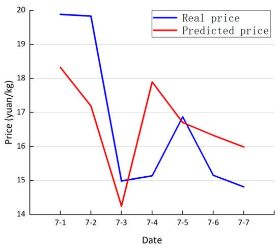
Figure 4.
Fitting effect diagram of aquatic rhizomes.
Table 4.
Next week’s pricing forecast table (CBY/kg).
Based on the statistics from Table 2 and Table 4, we calculated the predicted profit. Using the data on replenishment volume and pricing, we multiplied these values and summed the results for each product category. Consequently, our predicted profit stands at 20,698.99 CNY, while the actual profit of the supermarket is reported as 19,732.89 CNY. This represents an increase of 4.67% in our predicted profit compared to the actual profit, computed on a weekly basis. In an attempt to compare our model with alternative approaches, we applied ARIMA and other models for prediction. The profit predicted by these models amounted to 20,031.12 CNY, showing a rise of 3.23%. It is noteworthy that the predictions from other models substantially differed from the actual data, especially in terms of the replenishment figures for the six categories. This discrepancy suggests that these models may not adequately account for seasonal factors influencing replenishment volumes, leading to inconsistencies between predictions and reality. Consequently, these models may not accurately reflect real-world scenarios.
4.3. Prediction of Pricing and Replenishment Strategies for a Single Product
We use Lingo mathematical software (version 17.0) to solve the above model. The replenishment quantity and pricing strategy of a single product on July 1 are shown in Table 5. Based on the statistics provided in the table, we computed the projected profit and compared it with the actual profit of the supermarket. By multiplying the data on replenishment volume and pricing for each individual commodity and summing the results, we arrived at a predicted profit of 8259.57 CNY. However, the actual profit of the supermarket was 7832.16 CNY. This indicates that our predicted profit increased by 5.17% daily compared to the actual profit.
Table 5.
Replenishment volume and pricing strategy of a single item on 1 July.
5. Prospects and Suggestions
Based on the above discussions, it can be concluded that more profits are able to be made based on the proposed model and strategy. Although our current model considers various factors, there is still room for optimization. If fresh food supermarkets or related food institutions could collect more detailed and extensive data, our model would better align with reality and possess broader application prospects. We recommend that fresh food supermarkets consider collecting the following six types of data: Incorporating these data sources into our model will enable fresh food supermarkets to make more informed and adaptive decisions related to replenishment and pricing, thereby enhancing operational efficiency and customer satisfaction.
- (1)
- Consumer return tracking data
- Opinion: Conduct market survey questionnaires during consumers’ shopping check-out to gather feedback on their satisfaction with the shopping experience, related needs for commodity categories, and other relevant information. This data can assist supermarkets in making real-time adjustments to replenishment and pricing decisions.
- Reason: Consumer feedback can directly reflect the quality of service, product availability, product quality, and pricing decisions. Addressing these aspects can lead to improved business strategies for fresh supermarkets, attracting more customers, and creating a positive cycle for dynamic adjustments to replenishment and pricing.
- (2)
- Commodity consumption rate data
- Opinion: Collect comprehensive data on the attrition rates of vegetable commodities, considering various real-world factors that may affect consumption.
- Reason: Idealized consumption rates may not account for factors like residents’ inability to purchase vegetables on certain days or the absence of discounts. Preparing for unexpected situations by improving data on commodity attrition rates will aid supermarkets in adapting replenishment and pricing strategies under special circumstances.
- (3)
- Market demand data
- Opinion: Actively research market demand for vegetable commodities through surveys and interviews, collecting detailed data on consumer needs.
- Reason: Detailed market demand data can reveal specific consumer requirements for various vegetable categories. This information can significantly influence replenishment and pricing decisions, enabling supermarkets to respond to consumer needs by adjusting the quantity and pricing of goods.
- (4)
- Peer competition data
- Opinion: Gather information on promotional activities conducted by neighboring fresh food supermarkets and compile it into peer competition data.
- Reason: Nearby fresh food supermarkets often compete with each other for customers, leading to potential price wars on vegetable commodities. Price adjustments can affect sales volumes, impacting supermarket profits. Collecting peer competition data can help supermarkets make informed decisions on replenishment and pricing.
- (5)
- Weather data
- Opinion: Monitor and collect local weather forecasts for the upcoming week and organize this data.
- Reason: Weather conditions significantly influence the sales of vegetable commodities. Temperature changes can affect storage cycles and pricing, while precipitation can impact customer traffic and goods transportation. Given the unpredictability of weather, having access to weather data allows supermarkets to adjust replenishment and pricing decisions to mitigate economic losses.
- (6)
- Supply chain data
- Opinion: Gain insights into supply chain information, including inventory levels, supplier reliability, delivery times, and transportation times, and consolidate it into comprehensive supply chain data.
- Reason: Supply chain information plays a pivotal role in replenishment and pricing decisions. Inventory levels determine the extent of replenishment and pricing adjustments, while supplier reliability affects the timeliness of fresh supply. Integrating supply chain data enables supermarkets to fine-tune their replenishment and pricing strategies for vegetable goods.
6. Conclusions
This study employed a combination of models to address pricing and replenishment challenges in fresh food supermarkets. We used the Pearson correlation coefficient to analyze the relationship between total sales volumes of various vegetable categories and cost-plus pricing. For forecasting daily replenishments of six different vegetable types in the upcoming week, we employed seasonal ARIMA models. To enhance the reliability and accuracy of our results, we employed 0–1 integer programming after data filtration for individual product pricing and replenishment strategies. This paper provides a comprehensive exploration of commodity pricing and replenishment strategies, offering valuable insights and guidance for the management of retailers. However, this study has its limitations. When constructing seasonal ARIMA models based on time series periodicity and seasonality, we employed a few model parameters and did not consider multiple lag times, resulting in a certain degree of deviation. Future work will incorporate additional data sources, such as weather and supply chain data, as well as introduce multi-dimensional models to improve the robustness of our approach.
Author Contributions
Conceptualization, J.L. and B.L.; methodology, J.L.; software, J.L.; validation, J.L.; resources, J.L.; writing—original draft preparation, J.L.; writing—review and editing, J.L. and B.L.; visualization, J.L.; supervision, B.L. All authors have read and agreed to the published version of the manuscript.
Funding
This research received no external funding.
Data Availability Statement
The data are self-contained within this article.
Conflicts of Interest
The authors declare no conflict of interest.
Correction Statement
Due to an error in article production, incorrect references were previously listed in the main text. This information has been updated and this change does not affect the scientific content of the article.
References
- Chen, J.; Dan, B. Fresh agricultural product supply chain coordination under the physical loss-controlling. Eng.-Theory Pract. Syst. 2009, 29, 54–62. [Google Scholar]
- Emanuele, F.; Andrea, M.; Giuseppe, N.D. Vanilla-option-pricing: Pricing and market calibration for options on energy commodities. Softw. Impacts 2020, 6, 100043. [Google Scholar]
- Guo, L. Cross-border e-commerce platform for commodity automatic pricing model based on deep learning. Electron. Commer. Res. 2022, 22, 1–20. [Google Scholar] [CrossRef]
- Chen, J.; Ewald, C.; Ouyang, R.; Westgaard, S.; Xiao, X. Pricing commodity futures and determining risk premia in a three factor model with stochastic volatility: The case of Brent crude oil. Ann. Oper. Res. 2021, 313, 29–46. [Google Scholar] [CrossRef]
- Crosby, J.; Frau, C. Jumps in commodity prices: New approaches for pricing plain vanilla options. Energy Econ. 2022, 114, 106302. [Google Scholar] [CrossRef]
- Liang, X.; Wang, N.; Zhang, M.; Jiang, B. Bi-objective multi-period vehicle routing for perishable goods delivery considering customer satisfaction. Expert Syst. Appl. 2023, 220, 119712. [Google Scholar] [CrossRef]
- Reza, M.A.; Rashed, S.; Hassan, M.S.H. Optimizing the sales level of perishable goods in a two-echelon green supply chain under uncertainty in manufacturing cost and price. J. Ind. Prod. Eng. 2022, 39, 581–596. [Google Scholar]
- Zhao, S.; Li, W. Block chain-based traceability system adoption decision in the dual-channel perishable goods market under different pricing policies. Int. J. Prod. Res. 2023, 61, 4548–4574. [Google Scholar] [CrossRef]
- Zhao, H.; Wang, X. Basic pricing model of perishable goods by electric businesses under group buying in cooperation mode between merchants and group buying platform. J. Shenyang Univ. Technol. (Soc. Sci. Ed.) 2018, 11, 544–548. [Google Scholar]
- Zhang, X.; Mo, N. Ordering and Pricing Strategy of Perishable Goods Inventory Based on Weibull Function and Price Discount. J. Chongqing Norm. Univ. (Nat. Sci.) 2019, 37, 1–5. [Google Scholar]
- Guo, S. Dynamic Pricing of Perishable Goods with Consideration of Consumer Returns. Master’s Thesis, Nanjing University of Science and Technology, Nanjing, China, 2022. [Google Scholar]
- Young, H.C. Optimal pricing and ordering policies for perishable commodities. Eur. J. Oper. Res. 2003, 144, 68–82. [Google Scholar]
- Elmaghraby, W.; Gulcu, A.; Keskinocak, P. Designing opyimal preannounced markdowns in the presence of rational customers with multiunit demands. Manuf. Serv. Oper. Manag. 2008, 10, 126–148. [Google Scholar] [CrossRef]
- Aviv, Y.; Pazgal, A. Optimal pricing of seasonal products in the presence of forward looking consumers. Manuf. Serv. Oper. Manag. 2008, 10, 339–359. [Google Scholar] [CrossRef]
- Maihami, R.; Nakhai, K. Joint control of inventory and its pricing for noninstantaneously deteriorating items under permissible delay in payments and partial backlogging. Math. Comput. Model. 2012, 55, 1722–1733. [Google Scholar] [CrossRef]
- Wang, Y. Cost-plus pricing from KFC. Econ. Res. Guide 2011, 17, 1673-291X (2011) 17-0158-02. [Google Scholar]
- Cleophas, T.J.; Zwinderman, A.H. Bayesian Pearson Correlation Analysis. In Modern Bayesian Statistics in Clinical Research; Springer: Cham, Switzerland, 2018. [Google Scholar]
- Dimri, T.; Ahmad, S.; Sharif, M. Time series analysis of climate variables using seasonal ARIMA approach. J. Earth Syst. Sci. 2020, 129, 149. [Google Scholar] [CrossRef]
- Khashei, M.; Bijari, M.; Hejazi, S.R. Combining seasonal ARIMA models with computational intelligence techniques for time series forecasting. Soft Comput. 2012, 16, 1091–1105. [Google Scholar] [CrossRef]
- John, R.C.S. Applied linear regression. J. Qual. Technol. 1981, 13, 218–219. [Google Scholar] [CrossRef]
- Flatman, R.J.; Badrick, T.C. Linear regression. Aust. J. Med. Sci. 1992, 13, 13–17. [Google Scholar]
- Cornejo-Acosta, J.A.; García-Díaz, J.; Pérez-Sansalvador, J.C.; Segura, C. Compact Integer Programs for Depot-Free Multiple Traveling Salesperson Problems. Mathematics 2023, 11, 3014. [Google Scholar] [CrossRef]
- Wang, S.; Cheng, J.; Zhu, B. Optimal operation of a single unit in a pumping station based on a combination of orthogonal experiment and 0-1 integer programming algorithm. Water Supply 2022, 22, 7905–7915. [Google Scholar] [CrossRef]

Disclaimer/Publisher’s Note: The statements, opinions and data contained in all publications are solely those of the individual author(s) and contributor(s) and not of MDPI and/or the editor(s). MDPI and/or the editor(s) disclaim responsibility for any injury to people or property resulting from any ideas, methods, instructions or products referred to in the content. |
© 2023 by the authors. Licensee MDPI, Basel, Switzerland. This article is an open access article distributed under the terms and conditions of the Creative Commons Attribution (CC BY) license (https://creativecommons.org/licenses/by/4.0/).