The Influence of Demand Fluctuation and Competition Intensity on Advantages of Supply Chain Dominance

Abstract

We studied a supply chain consisting of multiple suppliers and multiple retailers. We use the Cournot–Stackelberg game, the Market–Stackelberg game, and the Market–Nash game to simulate the situation where the upstream seller’s market dominance power gradually decreases while the downstream buyer’s market power increases. The equilibrium decision and supply chain performance under the three models are compared and analyzed, as well as their responses to external market changes such as demand fluctuation and market competition intensity. The research shows that (1) in a seller-dominated supply chain, the increase in buyer power reduces market equilibrium production and wholesale price; (2) in the face of strong demand fluctuations, equivalent power between upstream and downstream can contribute to the stabilization of production and wholesale prices; (3) when market demand fluctuation is small, market power brings a higher profit level, and supply chain participants would like to actively compete for market power. However, when the demand fluctuates greatly, the profit advantage brought by market dominance is no longer significant, and there is no need to spend much to fight for market dominance; (4) the fierce competition of upstream suppliers will induce upstream to give up the competition for market dominance, and make the market power less attractive to downstream retailers. While the fierce horizontal competition downstream will stimulate both suppliers and retailers to actively compete for market power, (5) sufficient market competition will improve total supply chain profit, so encouraging competition is conducive to the overall economic development of society.

1. Introduction

According to the definition of El-Ansary and Stern [1], the power of a supply chain member is its ability to control the decision variables of other members of the supply chain. And the power differentials among supply chain members can be expressed indirectly through the game timing in supply chain games [2,3]. The first decisionmaker in the game influences the decisions of the later decisionmakers, thus creating its dominance. In this framework, a number of researchers have focused on the impact of dominance on supply chain performance [4,5,6]. And most of these studies are based on a “single-supplier, single-retailer” supply chain structure (there is also a reasonable amount of literature that examines the structure of “one supplier and two retailers” or “two suppliers and one retailer”). With the general advancement of globalization and the rapid development of e-commerce, the “multiple-suppliers, multiple-retailers” model of multiple suppliers providing products to multiple retailers through online direct selling or offline wholesaling is very popular [7]. The major difference between the above two models is that the latter introduces horizontal competition between suppliers (retailers). However, whether horizontal competition will break the profit advantage of the dominance is not very clear. In addition, much of the literature on the power structure of the supply chain is based on the reality that the rise of retail giants, such as Wal-Mart, continues to suppress suppliers in terms of wholesale prices, which may also affect consumer welfare. However, the shift of dominance from one party to another is a gradual process, and even Wal-Mart did not have dominance from the beginning of its operations. In reality, the non-dominant party may first undermine the dominant party’s power advantage in many ways. For example, Korpeoglu et al. [8] suggested that a retailer can influence wholesale prices by changing the purchasing budget to exercise its own buyer’s power and obtain a higher level of profit. Geylani et al. [9] developed a theoretical model to show how manufacturers strategically respond to dominant retailers. In these cases, the dominant party did not lose its dominance in terms of decision timing, but the non-dominant party undermined the dominant party’s power advantage through certain strategies. As the non-dominant party continues to grow, its power is further increased, resulting in equal status with the dominant party. For example, with the rapid development of Wal-Mart, Unilever gradually lost its dominant position in the supply chain, and the two formed an even situation. In current studies, modeling of the reality of this gradual decrease in dominance needs to be further explored.

Based on the above theories and motivations, we intend to extend the discussion of dominance advantage to “multiple-suppliers, multiple-retailers” supply systems and study the impact of the gradual weakening of suppliers’ dominance on the performance of supply chains and firms. The following questions are discussed through a comparative analysis of the equilibrium results under the three games:

In a “multiple-suppliers, multiple-retailers” supply system, does the party that prioritizes decisions still have a first-mover advantage?

Does competition between upstream suppliers (downstream retailers) affect the first-mover advantage? How?

Do fluctuations in market demand affect the first-mover advantage? How?

In a “multiple-suppliers, multiple-retailers” supply chain system, there is horizontal competition between suppliers (retailers) and vertical competition between suppliers and retailers. Suppliers (retailers) are substitutes, and there is no flow of goods in the horizontal competition. The study by Chen et al. [10] showed that the power structure of the vertical supply chain has a more significant impact on the financial performance of individual firms or the entire supply chain than the horizontal supply chain. In order to simplify the model without compromising the purpose of the study, we assume that the market power between suppliers (retailers) is equal and thus adopt the Cournot game model. Although the Cournot game was first applied to competition in oligopolistic markets, researchers have also applied it to games between multiple horizontal competitors with equal market power. For example, Corbett and Karmarkar [11] studied Cournot competition among multiple suppliers in a wholesale market. Roy et al. [12] focused on the application of the Cournot game to business activities by finding strategic decisions and equilibrium solutions to the C&K-based Cournot game. Cabolis et al. [13] studied the Cournot model of multiple oligopolies to capture the interplay between firms’ investment and merger decisions. Deo and Corbett [14] studied the effect of the number of competitors on participants’ decisions in a Cournot game under output uncertainty. Of course, there can be power imbalances between the same levels, and the interested reader is referred to some recent literature, such as the studies by Chakraborty et al. (2021) [15], Du et al. (2022) [16], etc.

In the flow of goods, there is vertical competition between suppliers and retailers, which is reflected in their opposing interests in wholesale prices. Vertical competition in a supply chain can be represented by the Stackelberg game and the Nash game, depending on market power. In the Nash game, both parties have equal power and make decisions at the same time [17,18,19]. And in the Stackelberg game, the market-dominant party has a first-mover advantage. Fang et al. have referred to vertical dominance as channel leadership [20]. In recent years, there has been much literature on vertical competition in supply chains, which adopts the Stackelberg game to reflect the power difference between upstream and downstream of the supply chain. For example, Jin et al. [21] studied the supply chain with suppliers as the dominant party, Pan Kewen et al. [22] studied the supply chain with downstream retailers as the dominant party, and the studies by Xue et al. [23] and Li et al. [24] consider the case of different power structures. In terms of the impact of dominance on profit, similar findings were obtained: the dominant party has the right to prioritize decision-making and, therefore, has a first-mover advantage to obtain a higher level of profit. However, some researchers argue that whether a firm can benefit from dominance is also influenced by factors such as the demand function, demand uncertainty [4,5], the price sensitivity coefficient [10,25], and so on.

Based on the above research, this paper models the process of gradually decreasing the dominance of upstream suppliers and gradually increasing the power of downstream retailers in the “multiple-suppliers, multiple-retailers” supply chain, using the Cournot–Stackelberg game, the Market–Stackelberg game, and the Market–Nash game. (1) In the Cournot–Stackelberg game, the suppliers have dominance over the supply chain. A horizontal Cournot game is played between suppliers (retailers), and a supplier-dominated Stackelberg game is played between suppliers and retailers. In this game, the supplier has the strongest supply chain dominance, such as the four international major grain merchants, the United States ADM, Bunge, Cargill, and France’s Louis Dreyfus, which control 80% of the world’s grain trading volume with grain pricing power. (2) In the Market–Stackelberg game, the supplier still has dominance in the supply chain, but the retailer can undermine the supplier’s dominance advantage by deciding on purchasing budgets. Korpeoglu et al.’s [8] research named it the Market game, and in this paper, in order to show both horizontal and vertical competition in supply chain systems, this game is referred to as the Market–Stackelberg game. The competition between some supermarket chains and strong brand suppliers is similar to this relationship: retailers such as Bravo, Home Depot, and Best Buy utilize their buyer power to obtain lower purchasing prices. (3) In the Market–Nash game, the power of supply chain members is balanced. All suppliers and retailers make decisions at the same time, and retailers still make purchasing budget decisions. Competition between general retail stores and non-branded suppliers is usually similar to this game, and it may also be the case between branded suppliers and retailers with comparable power. Further explanations of the three games can be found in the next section.

This paper also involves related research on market uncertainty. As early as the 1950s, Charnes et al. [26] began to study uncertainty optimization. In recent years, more and more scholars have studied the uncertainty problem from the perspectives of information [27], inventory [28], paths [29], and agricultural risk [30] in the supply chain, using different demand functions to characterize market demand. With reference to Ailawadi’s [31] view that the power structure and the timing of the game are affected by the way demand is modeled, this paper assumes that demand under the three games follows a random distribution to make the conclusions more general.

The papers of Shi et al., Wang et al., and Chen et al. are most similar to our study; they all studied the impact of dominance on supply chains based on a game-theoretic framework [4,5,6]. The study by Shi et al. [4] focused on a supply chain consisting of a retailer and a supplier under linear and isoelastic demand functions. They analyzed the Nash equilibrium of the three power structures: the supplier is absolutely dominant, the retailer is absolutely dominant, and the two have equal power. The results show that whether firms benefit from dominance depends on the form of the demand function: under linear demand, power-dominated firms are more profitable; under isoelastic demand, firms without dominance are more profitable. Wang et al. [5] extended the research framework of Shi et al. [4] but differed from their viewpoint of isoelastic demand counterparts. They adopted the retail margin percentage as the retailer’s decision variable in the retailer-dominated game in order to circumvent backward dominance. Chen et al. [6] constructed a supply chain game model consisting of one supplier and two retailers in order to study the competition among retailers.

The difference between our paper and the aforementioned studies lies in the following aspects. (1) In terms of research objectives, we focus on the effects of market competition intensity and market volatility on the dominant power advantage of supply chains. (2) In terms of modeling, we construct a “multiple-suppliers, multiple-retailers” supply chain system with demand uncertainty and simulate the competitive intensity of the market through the change in the number of suppliers and retailers. We model the end-market uncertainty through a stochastic distribution in order to eliminate the influence of the form of the demand function (linear or nonlinear) on the results. We use three game models to represent the gradual weakening of suppliers’ dominance: absolute dominance, diminished dominance, and equal dominance. (3) It can be seen that the conclusions in this paper differ significantly from the above literature. Our research finds that the dominant advantage of a supply chain does not necessarily always exist—in a “multiple-suppliers, multiple-retailers” supply system, it is also affected by demand fluctuations and competition. Only when demand volatility in the consumer market is small do participants’ profits increase with their supply chain’s dominant power. However, when demand volatility is high, the profit advantage from the dominant power of the supply chain is no longer significant, and none of the supply chain members have incentives to strive for market dominance. In terms of competition, if the number of upstream suppliers is high, leading to intense competition, dominant power does not lead to more profits for either suppliers or retailers. If the number of downstream retailers increases, resulting in more demanders in the wholesale market, dominant power is more profitable, and both suppliers and retailers are willing to strive aggressively for dominant power.

The remainder of this essay is structured as follows: First, for the process of gradually decreasing the power of upstream sellers, the Cournot–Stackelberg game, the Market–Stackelberg game, and the Market–Nash game under demand uncertainty is built, and the game equilibrium is computed. Next, the impact of market demand fluctuations on the supply chain dominance is compared. Finally, a comparison of the impact of supply chain competition intensity (number of suppliers or retailers) is performed.

2. Problem Description

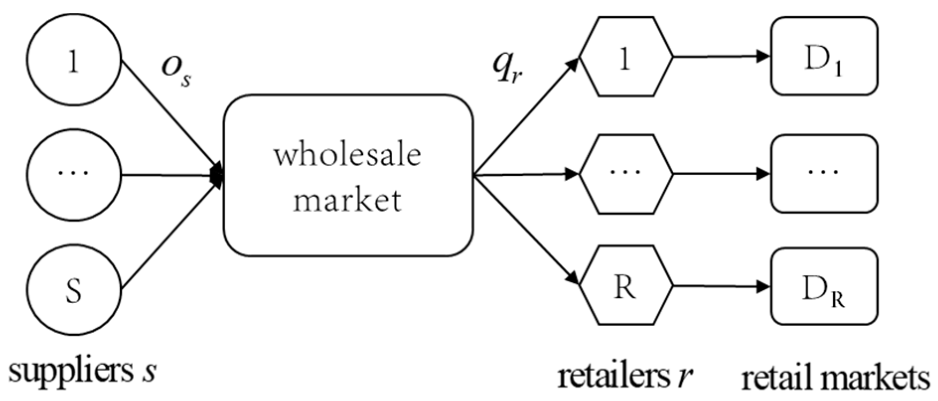
In this paper, we study the situation where multiple suppliers ($S$) supply multiple retailers ($R$) through the wholesale market under market uncertainty, as shown in Figure 1. We assume that each retailer ($r$) faces its own independent end-market whose demand ($D_r$) is uncertain and follows a distribution with a cumulative distribution function $F(x)$ and a probability density function $f(x)$. Note that the probability density function has an increasing generalized failure rate (IGFR), i.e., the demand function has the properties of the IGFR. This assumption stems from the reality that retailers in different cities or regions purchase products on the same wholesale market (online platform). All the horizontal competition mentioned in this paper is assumed to occur in the wholesale market: suppliers compete for demand, and the competitive pressure is reflected in selling; retailers compete for sources, and the competitive pressure is reflected in purchasing. At the same time, it is assumed that suppliers and retailers have complete information about each other and are both risk-neutral, pursuing their own profit maximization. For any retailer $r\in \{1,2,\dots ,R\}$, it procures an order quantity $q_r$ from the wholesale market at the wholesale price $w$ (then the total order quantity for all retailers is $Q={\displaystyle \sum _{r=1}^R{q}_r}$) and sells the product at the retail price $p$.

For suppliers, the unit cost of production is $c$, the quantity that the supplier $s\in \{1,2,\dots ,S\}$ sells to the wholesale market is $o_s$, and the total quantity produced is $O={\displaystyle \sum _{s=1}^S{o}_s}=o_s+O_{-s}$, where $O_{-s}$ denotes the total quantity produced by all suppliers except supplier $s$. In the wholesale market, we assume a market-clearing condition, where all products provided by suppliers are purchased by retailers, i.e., $Q={\displaystyle \sum _{r=1}^R{q}_r=}{\displaystyle \sum _{s=1}^S{o}_s}=O$. ${\pi }_s$ and ${\pi }_r$ denote the profits of supplier $s$ and retailer $r$, respectively. Then, we have:

$${\pi }_s=w{o}_s-c{o}_s$$

(1)

$${\pi }_r=pE\left[\min \left(D_r,q_r\right)\right]-w{q}_r$$

(2)

Then, the Cournot–Stackelberg, the Market–Stackelberg, and the Market–Nash games are used to simulate the game process of changing dominance between upstream suppliers and downstream retailers. The Sequence of events in these games is shown in Figure 2, and the specific explanation will be discussed in the next section.

3. Modeling

In this paper, the superscript * denotes the best response function; the superscripts C, M, and N denote the Cournot–Stackelberg game, the Market–Stackelberg game, and the Cournot–Nash game models, respectively; and the subscripts s and r denote the supplier and the retailer, respectively.

3.1. A Cournot–Stackelberg Game Model Where the Seller Is Dominant

In the supplier-dominated Cournot–Stackelberg game, there is Cournot competition among suppliers and among retailers. However, suppliers have more market power and a first-mover advantage, so the Stackelberg game is played between suppliers and retailers. Their game timeline is shown in Figure 2. In the first stage of decision-making, each supplier determines a production quantity by anticipating order quantities of retailers and its impact on wholesale price. Then, at the end of the first stage, the anticipated wholesale price is generated from market-clearing conditions. In the second stage, each retailer determines an order quantity by taking the wholesale price as given. Once production and purchases are determined separately, the market price can be determined according to the market clearing conditions. The decision-making goals of both retailers and suppliers are to maximize their expected profits. The expected profit functions of the supplier and the retailer are expressed as follows:

$$\max {\pi }_s^C=\max \left(w{o}_s-c{o}_s\right)\hspace{1em}s.t.O_{-s}+o_s={\displaystyle \sum _{r=1}^R{q}_r}$$

(3)

$$\max \left({\pi }_r^C\right)=\max \left(pE\left[\min (D_r,q_r)\right]-w{q}_r\right)$$

(4)

Nash equalization strategies are solved by backward induction, as shown in

Table 1. Comparison of equilibrium solutions and members’ profits under three games.

Parameters	C–S Game	M–S Game	M–N Game
Expression for equilibrium order quantity	$F(q_r^C)+\frac{q_r^{C}f(q_r^C)}{S}=1-\frac{c}{p}$	$F(q_r^M)+\frac{q_r^{M}f(q_r^M)}{S}=1-\frac{R}{R-1}\frac{c}{p}$	$F(q_r)=1-\frac{cRS}{p(R-1)(S-1)}$
Production quantity	$o_s^{C*}=\frac{R}{p}\cdot \frac{p\left(1-F(q_r^C)\right)-c}{f(q_r^C)}$	$o_s^{M*}=\frac{R}{p}\cdot \frac{p\left(1-F(q_r^M)\right)-\frac{R}{R-1}c}{f(q_r^M)}$	$o_s^{N*}=\frac{R}{S}{q}_r^N$
Wholesale price	$w^{C*}=\frac{p}{S}f(q_r^C)q_r^C+c$	$w^{M*}=\frac{R-1}{SR}pf(q_r^M)q_r^M+c$	$w^{N*}=\frac{Sc}{S-1}$
Supplier’s profit	${\pi }_s^{C*}=\frac{Rpf(q_r^C){(q_r^C)}^2}{S^2}$	${\pi }_s^{M*}=\frac{(R-1)pf(q_r^M)}{S^2}{(q_r^M)}^2$	${\pi }_s^{N*}=\frac{cR}{S(S-1)}{q}_r^N$
Retailer’s profit	$\begin{array}{c}{\pi }_r^{C*}=\left(p-\frac{p}{S}f(q_r^C)q_r^C-c\right)q_r^C\\ -p{\displaystyle {\int }_0^{q_r^C}F(x)dx}\end{array}$	$\begin{array}{c}{\pi }_r^{M*}=\left(p-\frac{R-1}{SR}pf(q_r^M)q_r^M-c\right)q_r^M\\ -p{\displaystyle {\int }_0^{q_r^M}F(x)dx}\end{array}$	$\begin{array}{c}{\pi }_r^{N*}=\left(p-\frac{Sc}{S-1}\right)q_r^N\\ -p{\displaystyle {\int }_0^{q_r^N}F(x)dx}\end{array}$

. In the Nash equilibrium of this game, no supplier has an incentive to change his production quantity, and no retailer has an incentive to change her order quantity.

Proof. 

The retailer first determines the functional relationship between the ordering quantity and the wholesale price according to the principle of profit maximization, which can be obtained from the Equation $\frac{\partial E\left({\pi }_r^C\right)}{\partial q_r}=p-w-pF\left(q_r\right)=0$ for $q_r=F^{-1}\left(\frac{p-w}{p}\right)$ and the wholesale price $w=p\left(1-F\left(q_r\right)\right)$. On the basis of market clearing, there is an equilibrium total production equal to the equilibrium total order quantity, i.e., $o_s+O_{-s}=R{q}_r=R{F}^{-1}\left(\frac{p-w}{p}\right)$, and there is $o_s=R{F}^{-1}\left(\frac{p-w}{p}\right)-O_{-s}$. The supplier then determines the optimal production quantity based on the corresponding functional relationship between the retailer’s order quantity and the wholesale price. Substituting $o_s=R{F}^{-1}\left(\frac{p-w}{p}\right)-O_{-s}$ into Equation (3) and taking a first-order derivative of the wholesale price, the supplier’s optimal production quantity $o_s^{C*}=\frac{R}{p}\cdot \frac{p\left(1-F(q_r^C)\right)-c}{f(q_r^C)}$ is obtained, and the optimal wholesale price is calculated as $w^{C*}=\frac{p}{S}f(q_r^C)q_r^C+c$. The proof is complete. □

3.2. A Market–Stackelberg Game Model Where the Seller’s Dominance Erosion

The biggest difference between the Market–Stackelberg game and the Cournot–Stackelberg game is that the retailer, as a follower, changes the decision variable from purchasing quantity to purchasing budget. The purchasing budget information is then used to influence the supplier’s decision. The game timeline is shown in Figure 2. In the first stage of decision-making, each supplier determines its production quantity by considering its impact on the wholesale price, and in the second stage, each retailer determines its procurement budget by considering its impact on the wholesale price. The wholesale price is determined according to the total procurement budget and the total production, while each retailer’s order quantity is determined by its procurement budget and the equilibrium wholesale price. Denote the procurement budget of the retailer $r\in \{1,2,\dots ,R\}$ by $b_r$ and denote the budget of all retailers by $B={\displaystyle \sum _{r=1}^R{b}_r}=b_r+B_{-r}$, where $B_{-r}$ is the total purchasing budget of all retailers except the retailer $r$. Then, we can write the wholesale price $w$ and retailer r’s order quantity $q_r$ as follows:

$$w=\frac{B}{O}=\frac{b_r+B_{-r}}{O}={\displaystyle \sum _{r=1}^R{b}_r}/{\displaystyle \sum _{s=1}^S{o}_s}$$

(5)

$$q_r=\frac{b_r}{w}=\frac{b_r}{B}O=\frac{b_r}{b_r+B_{-r}}O$$

(6)

At this point, the optimization problem for suppliers and retailers is:

$$\max {\pi }_s^M=\max \left(w{o}_s-c{o}_s\right)\hspace{1em}s.t.w=\frac{B}{O_{-s}+o_s}$$

(7)

$$\max {\pi }_r^M=\max \left(pE\left[\min (D_r,q_r)\right]-w{q}_r\right)\hspace{1em}s.t.w=\frac{B_{-r}}{O-q_r}$$

(8)

The solution using backward induction leads to the equilibrium decisions of the members under the Market–Stackelberg game, as shown in Table 1.

Proof. 

Firstly, from Equations (5) and (6), the derivation of $b_r$ is obtained as $\frac{\partial q_r}{\partial b_r}=\frac{O{B}_{-r}}{{\left(b_r+B_{-r}\right)}^2}$. Secondly, the expressions of $q_r$ and $w$ are substituted into the expected profit function of the retailer, and the optimal purchasing budget is obtained as $b_r^{M*}=\frac{B\left(B-Op+OpF(q_r)\right)}{Op\left(F(q_r)-1\right)}$ by making $\frac{\partial E\left({\pi }_r^M\right)}{\partial b_r}=0$. According to Equation (5), the expression of the wholesale price can be written as $w^{M*}=\frac{R-1}{R}p(1-F(q_r^M))$. Then, the supplier, considering his own benefit maximization, performs the first-order derivation of the production quantity $o_s$, and the optimal production quantity is derived as $o_s^{M*}=\frac{R}{p}\cdot \frac{p\left(1-F(q_r^M)\right)-\frac{R}{R-1}c}{f(q_r^M)}$ by making $\frac{\partial {\pi }_s^M}{\partial o_s}=0$. Finally, the equilibrium solution is substituted into the profit expression, and the profits of supplier $s$ and retailer $r$ can be obtained (see Table 1). The proof is complete. □

3.3. A Market–Nash Game Model with Power Equilibrium between Sellers and Buyers

Unlike the previous two games, in a Market–Nash game, the retailer and the supplier make decisions on purchasing budget and production quantity at the same time, respectively (see Figure 2). Therefore, no one has a first-mover advantage. To solve the Market–Nash problem, we only need to take the first-order derivatives of the objective functions (7) and (8) in the previous Market–Stackelberg model with respect to the purchasing budget $b_r$ and the production quantity $o_s$, respectively. Then, make the first-order derivative solution equal to 0, i.e., $\frac{\partial {\pi }_r^N}{\partial b_r}=0$ and $\frac{\partial {\pi }_s^N}{\partial o_s}=0$, and solve the problem in conjunction with each other to obtain $b_r^{N*}=\frac{cS}{S-1}{F}^{-1}\left(1-\frac{cRS}{\left(R-1\right)\left(S-1\right)p}\right)$ and $o_s^{N*}=\frac{R}{S}{F}^{-1}\left(1-\frac{cRS}{\left(R-1\right)\left(S-1\right)p}\right)$. So, we obtain the optimal wholesale price $w^{N*}=\frac{cS}{S-1}$ and the order quantity $q_r^{N*}=F^{-1}\left(1-\frac{cRS}{p(R-1)(S-1)}\right)$.

3.4. Comparative Analysis of Game Equilibrium Solutions

In order to compare and analyze the differences in supply chain strategies under the three games, the above equilibrium solutions $w^{*}$, $o_s^{*}$, and $q_r^{*}$ are substituted into the corresponding profit expressions to obtain the optimal profits for suppliers and retailers, as shown in Table 1. For the sake of brevity, the Cournot–Stackelberg game, the Market–Stackelberg game model, and the Market–Nash game is abbreviated as the C–S game, M–S game, and M–N game, respectively.

Based on the above results, the following proposition is obtained:

Proposition 1. 

In a “multiple-suppliers, multiple-retailers” supply chain ($S\ge 2,R\ge 2$), the retailer’s order quantity decision satisfies:

(1)

The expressions for the retailer’s equilibrium order quantity under C–S, M–S, and M–N games are $F(q_r^C)+\frac{q_r^{C}f(q_r^C)}{S}=1-\frac{c}{p}$, $F(q_r^M)+\frac{q_r^{M}f(q_r^M)}{S}=1-\frac{Rc}{\left(R-1\right)p}$, and $F(q_r^N)=1-\frac{cRS}{p(R-1)(S-1)}$, respectively;

(2)

The retailer’s equilibrium order quantity in the M–S game is constantly smaller than that in the C–S game, i.e., $q_r^{M*}<q_r^{C*}$;

(3)

Retailer’s order quantity is positively related to the number of suppliers under all three games, and, with the exception of the C–S game, order quantity is also positively related to the number of retailers.

Proof. 

Demand satisfies the generalized incremental failure rate (IGFR), i.e., $\frac{f(.)}{1-F(.)}$ is an increasing function, so we can obtain that:

$$f^{\prime }(x)+\frac{f^2(x)}{1-F(x)}>0$$

(9)

According to the expressions of equilibrium order quantity $F(q_r^C)+\frac{q_r^{C}f(q_r^C)}{S}=1-\frac{c}{p}$ and $F(q_r^M)+\frac{q_r^{M}f(q_r^M)}{S}=1-\frac{Rc}{\left(R-1\right)p}$, it is clear that $F(q_r^{.})+\frac{q_r^{.}f(q_r^{.})}{S}<1$ (note that $q_r^{.}$ refers to either $q_r^C$ or $q_r^M$), i.e.,

$$\frac{q_r^{.}f(q_r^{.})}{S(1-F(q_r^{.}))}<1$$

(10)

Set $\mathrm{\Omega }(q_r^{.})=F(q_r^{.})+\frac{q_r^{.}f(q_r^{.})}{S}$, then we have $\frac{\partial \mathrm{\Omega }(q_r^{.})}{\partial q_r^{.}}=f(q_r^{.})+\frac{f(q_r^{.})}{S}+\frac{q_r^{.}{f}^{\prime }(q_r^{.})}{S}$. Perform a simple substitution, and then we obtain $\frac{\partial \mathrm{\Omega }(q_r^{.})}{\partial q_r^{.}}=f(q_r^M)\left(1-\frac{q_r^{.}f(q_r^{.})}{S\left(1-F(q_r^{.})\right)}\right)+\frac{q_r^{.}}{S}\left(f^{\prime }(q_r^{.})+\frac{f^2(q_r^{.})}{1-F(q_r^{.})}\right)+\frac{f(q_r^{.})}{S}$. Using inequalities (9) and (10), it is easy to observe that $\frac{\partial \mathrm{\Omega }(q_r^{.})}{\partial q_r^{.}}>0$. Thus, $\mathrm{\Omega }(q_r^{.})$ is an increasing function on $q_r^{.}$. And since $\mathrm{\Omega }(q_r^C)=1-\frac{c}{p}>\mathrm{\Omega }(q_r^M)=1-\frac{Rc}{\left(R-1\right)p}$, we have $q_r^{C*}>q_r^{M*}$. Proposition 1-(2) is proved.

In the C–S and M–S games, the expressions of equilibrium order quantity are $F(q_r^C)+\frac{q_r^{C}f(q_r^C)}{S}=1-\frac{c}{p}$ and $F(q_r^M)+\frac{q_r^{M}f(q_r^M)}{S}=1-\frac{Rc}{\left(R-1\right)p}$, respectively. Since $\mathrm{\Omega }(q_r^{.})$ is an increasing function with respect to $q_r^{.}$, then for the given parameters c and p, it is clear that a larger $S$ corresponds to a larger $q_r^{.}$, i.e., $q_r^{.}$ is increasing with respect to $S$. And according to the inverse function and implicit function derivation laws, $\frac{\partial q_r^N}{\partial S}=\frac{1}{f(q_r^N)}\frac{cRS}{p(R-1)}\frac{1}{{(S-1)}^2}>0$ holds in the M–N game. Therefore, in all three games, the retailers’ order quantity is positively related to the number of suppliers. Similarly, in the M–S and M–N games, according to the inverse function and implicit function derivation rule, we can get $\frac{\partial q_r^{M*}}{\partial R}=\frac{1}{{\mathrm{\Omega }}^{\prime }(q_r^{M*})}\frac{c}{{\left(R-1\right)}^{2}p}>0$, $\frac{\partial q_r^{N*}}{\partial R}=\frac{1}{F^{\prime }(q_r^{N*})}\frac{cS}{{\left(R-1\right)}^{2}p(S-1)}>0$. That is, the order quantity is also positively related to the number of retailers. In the C–S game, on the other hand, the equilibrium solution clearly shows that there is no relationship between the ordering quantity and the number of retailers. Propositions 1-(3) are proved. □

Since retailers face end markets with independent and identically distributed demand, their order quantity equals the amount of product flowing into the end market. From Propositions 1-(2), the dominant power of suppliers in the supply chain affects the products flowing into the end market. When retailers use a budget as a decision variable to constrain the dominance of suppliers, it reduces the total product inflow to the end market. Propositions 1-(3) show that when the supplier is absolutely dominant, changes in the number of retailers do not affect the equilibrium order quantity of each retailer. In contrast, when the supplier’s dominance becomes progressively weaker, an increase in the number of retailers stimulates each retailer to raise the equilibrium order quantity. This finding provides management insights for suppliers: when supplier dominance is weakened, they can buffer the negative impact of weakened power by aggressively exploring new markets to increase pressure on existing retailers and stimulate retailers to increase their order quantity.

Proposition 2. 

In a “multiple-suppliers, multiple-retailers” supply chain ($S\ge 2,R\ge 2$), the supplier’s production quantity decision satisfies:

(1)

Under the C–S, M–S, and M–N games, the supplier’s optimal production is $o_s^{C*}=\frac{R}{p}\cdot \frac{p\left(1-F(q_r^C)\right)-c}{f(q_r^C)}$, $o_s^{M*}=\frac{R}{p}\cdot \frac{p\left(1-F(q_r^M)\right)-\frac{R}{R-1}c}{f(q_r^M)}$, and $o_s^{N*}=\frac{R}{S}{q}_r^N$, respectively;

(2)

The supplier’s production in the M–S game is constantly smaller than that in the C–S game, i.e., $o_s^{M*}<o_s^{C*}$;

(3)

In all three games, a supplier’s production is positively related to the number of retailers and negatively related to the number of suppliers.

The proof is the same as the proof of Proposition 1, so the proof is omitted.

From Proposition 2, total output and total order quantity are equal due to the equilibrium of supply and demand in the wholesale market, so Proposition 2-(2) corresponds to Proposition 1-(2). They both show that the retailer’s use of budget decisions to weaken the supplier’s dominant power will reduce the total equilibrium output (total product inflow to the market). Proposition 2-(3) shows that regardless of whether the supplier has dominant power or not, he must increase output whenever he predicts an increase in the number of retailers and decrease output when he predicts an increase in suppliers.

Proposition 3. 

In a “multiple-suppliers, multiple-retailers” supply chain ($S\ge 2,R\ge 2$), the wholesale price decision satisfies:

(1)

Under the C–S, M–S, and M–N games, the optimal wholesale prices are $w^{C*}=\frac{p}{S}f(q_r^C)q_r^C+c$, $w^{M*}=\frac{R-1}{R}\frac{p}{S}f(q_r^M)q_r^M+c$, and $w^{N*}=\frac{Sc}{S-1}$, respectively;

(2)

The wholesale market price in the M–S game is constantly smaller than that in the C–S game, i.e., $w^{M*}<w^{C*}$;

(3)

In contrast to the C–S and M–N games, the wholesale price $w$in the M–S game is jointly determined by the supplier’s production decision and the retailer’s ordering decision.

Proof omitted.

A comparison of Proposition 3-(1) and Proposition 1-(1) shows that neither the retailer’s equilibrium order quantity nor the market equilibrium price is affected by the number of retailers in the C–S game. This is because retailers’ end markets are independent, and suppliers have no capacity constraints. Thus, despite an increase in the number of retailers, the supplier is always able to supply production that matches demand and thus cannot affect the wholesale price. Proposition 3-(2) shows that the wholesale market price in the M-S game is smaller than in the C–S game, indicating that the retailer can indeed benefit from using budget as a decision variable to obtain a lower wholesale price. The M–S game describes a common scenario in the marketplace: a retailer purchases products in the wholesale market and bargains with the supplier based on a limited budget, which reflects the retailer’s buyer power. However, it is not the case that an increase in retailer power necessarily affects the wholesale price in the M–N game. For example, the wholesale price is only related to the number of suppliers and the cost of production, despite the fact that the retailer acquires the same market power as the suppliers. Proposition 3 reveals this management insight: when the retailer has no market power at all, appropriate market power can achieve lower purchasing prices for it. And when the retailer has considerable power, it is difficult to use its power advantage to depress the purchasing price, and the effective way to reduce the purchasing price is to seek more sources of supply and encourage more suppliers to join the market.

Synthesizing Propositions 1, 2, and 3, it can be found that the relationship between equilibrium decision-making and power structure in a “multiple-suppliers, multiple-retailers” supply chain is different from in a “single-supplier, single-retailer” supply chain. In Shi et al.’s [4] study of the impact of power structure on the “single-supplier, single-retailer” supply chain, they concluded that the wholesale price (order quantity) increases (decreases) with the power of the supplier and decreases (increases) with the power of the retailer. In a “multiple-suppliers, multiple-retailers” system, wholesale prices and order quantity do not behave in this absolutely monotonous manner as supplier or buyer power changes. In a “multiple-suppliers, multiple-retailers” system, the strength of the power structure’s influence on the equilibrium decision is heavily influenced by market volatility and competition intensity.

Based on the above analysis of the equilibrium solution, given the complexity of the model, we will next use numerical experiments to analyze the decisions and supply chain performance of the three games in the face of changes in external factors, such as demand fluctuations and competition intensity.

4. The Impact of Demand Volatility on Dominance Advantages

To investigate the differences in strategies under different games, we conducted a numerical test using MATLAB tools. According to the equilibrium solution of Table 1, we fix $D_r\sim N\left(30,{20}^2\right)$, $R=5$, $S=10$, $p=3$, $c=1$.

4.1. Equilibrium Production and Wholesale Prices

Market demand volatility will affect firms’ business decisions because high demand uncertainty implies high mismatch costs. Centralized supply chains always benefit from reduced demand uncertainty. However, when considering the strategic interactions between supply chain members, it is not clear how the reduction in demand uncertainty affects the performance of supply chain members [28]. Therefore, this section examines how demand volatility affects the decision-making of supply chain members in different power situations.

Changing the standard deviation $\sigma$ from 5 to 50 to generate more instances for sensitivity analysis, we find that: (a) As shown in Figure 3a, equilibrium production changes the most in the C–S game (where the seller has more power) and the least in the M–N game (where buyer and seller have the same power). It can be seen that when sellers dominate, market volatility can have a significant impact on supply chain output, which means that sellers’ prioritized decision-making power promotes the bullwhip effect on the supply chain. And when the seller’s dominance diminishes, the impact of this volatility diminishes. (b) As shown in Figure 3b, the equilibrium wholesale price falls sharply under both the C–S and M–S models as market volatility increases, and the change is greatest under the C–S model. However, there is essentially no change under the M–N model.

To summarize, in the face of changes in market volatility, equilibrium production and price are more variable in the C–S model, smaller in the M–S model, and more stable in the M–N model. Besides, the supplier’s dominant power advantage, which is reflected in the wholesale price advantage, is more pronounced when the market is less volatile. Instead, it will put suppliers at a disadvantage when the market is more volatile, as too much supply can lead to plummeting prices and reduced revenues.

4.2. Profitability of Supply Chain Members

There has been much literature analyzing the impact of demand volatility on the profits of supply chain members under a certain game. It is generally recognized that suppliers benefit from reduced demand volatility, while retailers do not necessarily [4,32]. Therefore, this paper focuses on the impact of demand volatility on supply chain power advantages, i.e., it examines how profit advantages due to structural power are disturbed by demand fluctuations.

(1)

First, observe the change in the supplier’s profit, as shown in Figure 4a. When demand volatility is low, the supplier’s profit is maximized in the C–S game and minimized in the M–N game, i.e., the supplier’s profit decreases as their power diminishes. As demand volatility increases, the supplier’s profit in the M–N game gradually approaches those of the C–S and M–S games and later exceeds those of the M–S game. It can be seen that when demand volatility is high, dominant power cannot bring higher profits to suppliers, so it is not meaningful for suppliers to acquire larger market power.

(2)

Then, observe the change in the retailer’s profit, as shown in Figure 4b. When demand volatility is low, the retailer’s profit is maximized in the M–N game (where the retailer has more power) and minimized in the C–S game, i.e., the retailer’s profit increases as its power increases. When demand is more volatile, the results are the opposite. It can be seen that when demand volatility is high, it is not meaningful for retailers to acquire larger market power.

(3)

The trend in total supply chain profit is similar to that of retailers, but in general, the change is not significant.

To summarize, when market demand is less volatile, members’ profits increase as their supply chain dominance increases. Thus, suppliers will spend more to maintain their supply chain dominance, and retailers will invest more to gain buyer power. However, when the demand is more volatile, the gap between the profits in the three games decreases significantly, i.e., the profit advantage brought by the dominant power of the supply chain is no longer significant. Thus, none of the supply chain members have incentives to strive for market dominance.

5. The Effect of Competition Intensity on the Dominance Advantages

With the growth of e-commerce, more suppliers and retailers are joining the supply chain. The power advantage of supply chain structure in the presence of multiple supply chain members is also investigated. This section simulates the intensity of competition in the market by varying the number of retailers and suppliers and observes decisions and profitability characteristics in the supply chain.

5.1. Equilibrium Strategies for Supply Chains

Through programming, we summarize the effect of the number of supply chain members on supply chain equilibrium strategies under the three games, as shown in

Table 2. Equilibrium strategies for three games when the number of supply chain members increases.

	C–S Game		M–S Game		M–N Game
	$\mathit{S}$	$\mathit{R}$	$\mathit{S}$	$\mathit{R}$	$\mathit{S}$	$\mathit{R}$
Equilibrium production	↘	↗	↘	↗	↘	↗
Equilibrium order quantity	↗	—	↗	↗	↗	↗
Equilibrium wholesale price	↘	—	↘	↗	↘	—

↘, ↗ and—denote increasing, decreasing and constant, respectively.

. (1) First, analyze the equilibrium productions. The trend in output decision change with the number of supply chain members is the same under all three games; specifically, the output decreases with the number of suppliers and increases with the number of retailers. (2) Then, analyze the equilibrium order quantity. Equilibrium order quantity is not affected by the number of retailers only when the supplier is absolutely dominant. In all other cases, an increase in the intensity of competition raises the equilibrium order quantity and the amount of product in the end market. (3) Afterwards, analyze the equilibrium wholesale price. When the number of suppliers increases, the wholesale price decreases in all three games, which shows that the decreasing trend of the wholesale price with the increase in the number of suppliers is not affected by the power structure. And when the number of retailers changes, the changes in wholesale prices under different power structures show different trends. In the C–S and M–N games, the number of retailers does not affect the wholesale price, while in the M–S game, the wholesale price rises with the number of retailers.

5.2. Suppliers’ Profit

The intensity of upstream competition and the intensity of downstream competition can have different impacts on suppliers’ profits and their attitudes toward dominant power.

When the number of suppliers increases, as shown in Figure 5a, the intensity of upstream competition increases and the profit of suppliers in all three games decreases significantly. When the number of suppliers is small, suppliers’ profits are highest in the C–S game (where suppliers have more market power) and lower and very close in the M–S and M–N games. When the number of suppliers is large, the suppliers’ profits under the three games are basically the same. It can be seen that supply chain participants have no incentive to strive for market power when the intensity of competition is high.

When the number of retailers increases, as shown in Figure 5b, the profit of suppliers in all three games increases significantly. When the number of retailers is large, the suppliers make more profits in a game where they have more market power. Therefore, when downstream competition is fierce, suppliers will strive for supply chain dominance. This result is intuitive because, in our model, downstream retailers face independent demand markets, so an increase in the number of retailers is equivalent to opening up new markets and an increase in aggregate demand, prompting retailers to compete more aggressively in the purchasing market. In other words, expanding into new markets can be more profitable for suppliers who are dominant in the supply chain. There are real-world examples to verify this. Producers of high-value consumer goods, such as automobiles, computers, cell phones, etc., are generally vertically dominant, and these firms always tend to open up new markets to sell these products around the world.

In summary, intense horizontal competition within the upstream leads to negative attitudes toward supply chain dominance among upstream members, while intense horizontal competition within the downstream promotes competition for supply chain dominance among upstream members.

5.3. Profitability of Retailers

The intensity of upstream competition and downstream competition also have different impacts on retailers’ profits and their attitudes toward dominance in the supply chain.

When the number of suppliers increases, as shown in Figure 6a, the intensity of upstream competition increases, and the profit of retailers in all three games increases significantly. When the number of suppliers is small, retailers’ profits are highest in the M–N game, followed by the M–S game, and lowest in the C–S game. When the number of suppliers is large, the retailers’ profits under the three games are basically the same. It can be seen that retailers have no incentive to strive for market power when the intensity of upstream competition is large.

When the number of retailers increases, as shown in Figure 6b, retailers’ profits increase significantly in the M–N game, increase and then decrease in the M–S game, and are minimized in the C–S game. That is, when horizontal competition among retailers is intense, pursuing buyer power can enhance profit levels because when upstream competition is intense, sellers have greater selling pressure that would eliminate the advantage of dominant power in the supply chain, and retailers have no incentive to strive for market power. When downstream competition is intense, buyers have greater purchasing pressure. Moreover, supplies with dominance in the supply chain would hurt retailers’ profits even more, so gaining market power allows retailers to mitigate this pressure.

In summary, when the number of suppliers varies, retailers’ profits are essentially the same under all three games, and therefore, changes in the number of suppliers have little incentive for retailers to change the market power structure. The opposite result occurs when the number of retailers changes. When the retailer’s competition is intense, the retailer earns the highest profit in the M–N game, much higher than in the other two games. As a result, retailers are willing to pay a higher price for market dominance to significantly increase their profits.

5.4. Total Supply Chain Profit

Considering the sum of the profits of the S suppliers and R retailers in the supply chain as the total supply chain profit, the total profit under all three games can be denoted by $\mathrm{\Pi }={\displaystyle \sum _{s=1}^S{\pi }_s}+{\displaystyle \sum _{r=1}^R{\pi }_r}$. Investigating the variation of total supply chain profit with respect to the intensity of horizontal competition, we obtain Proposition 4.

Proposition 4. 

Total supply chain profit increases with the number of suppliers and retailers under all three games, i.e., $\frac{\partial {\mathrm{\Pi }}^{.}}{\partial S}>0$ and $\frac{\partial \mathrm{\Pi }}{\partial R}>0$.

Proof of Proposition 4. 

Referring to Table 1, the total supply chain profit in the equilibrium solutions of the C-S game is

$${\mathrm{\Pi }}^C={\displaystyle \sum _{s=1}^S{\pi }_s^C}+{\displaystyle \sum _{r=1}^R{\pi }_r^C}=\frac{Rpf(q_r^C){(q_r^C)}^2}{S}+R\left(p-\frac{p}{S}f(q_r^C)q_r^C-c\right)q_r^C-Rp{\displaystyle {\int }_0^{q_r^C}F(x)dx}=R(p-c)q_r^C-Rp{\displaystyle {\int }_0^{q_r^C}F(x)dx}$$

Taking the first-order derivative of this expression with respect to the number of suppliers S, we obtain

$$\frac{\partial {\mathrm{\Pi }}^C}{\partial S}=\frac{\partial {\mathrm{\Pi }}^C}{\partial q_r^C}\frac{\partial q_r^C}{\partial S}=R(p-c)\frac{\partial q_r^C}{\partial S}-RpF(q_r^C)\frac{\partial q_r^C}{\partial S}=R(p-c-pF(q_r^C))\frac{\partial q_r^C}{\partial S}$$

According to Table 1, $F(q_r^C)+\frac{q_r^{C}f(q_r^C)}{S}=1-\frac{c}{p}\Rightarrow F(q_r^C)<1-\frac{c}{p}$, therefore, $\frac{\partial {\mathrm{\Pi }}^C}{\partial q_r^C}=R(p-c-pF(q_r^C))>0$. According to Proposition 1-(3), $\frac{\partial q_r^C}{\partial S}>0$, therefore, $\frac{\partial {\mathrm{\Pi }}^C}{\partial S}=\frac{\partial {\mathrm{\Pi }}^C}{\partial q_r^C}\frac{\partial q_r^C}{\partial S}>0$.

Similarly, in the equilibrium solutions of the M-S and M-N games, ${\mathrm{\Pi }}^M=R(p-c)q_r^M-Rp{\displaystyle {\int }_0^{q_r^M}F(x)dx}$, ${\mathrm{\Pi }}^M=Rp{q}_r^N-Rp{\displaystyle {\int }_0^{q_r^N}F(x)dx}$. So, it can be easily derived that $\frac{\partial {\mathrm{\Pi }}^M}{\partial S}>0$ and $\frac{\partial {\mathrm{\Pi }}^N}{\partial S}>0$.

Similarly, it can be proved that $\frac{\partial {\mathrm{\Pi }}^C}{\partial R}>0$, $\frac{\partial {\mathrm{\Pi }}^M}{\partial R}>0$ and $\frac{\partial {\mathrm{\Pi }}^N}{\partial R}>0$.

Proposition 4 suggests that competition contributes to an increase in the total welfare of society and, therefore, encouraging competition is beneficial to the overall economic development of society. It is worth noting, however, that the increase in total welfare resulting from increased competition in the market is unevenly distributed between suppliers and retailers. In conjunction with the analysis in 5.1—5.3, (a) retailers are the biggest beneficiaries if there is intense competition on the supply side (an increase in the number of suppliers) (see Figure 5a and Figure 6a). Not only is the increase in welfare due to competition captured by the retailers, but they also take a portion of the profits originally held by the suppliers. This is because, as shown in Table 2, an increase in the number of suppliers not only leads to a lower wholesale price but also induces each supplier to reduce its output, which results in a higher loss of profit for the supplier. (b) In the case of high competition on the retail side (increase in the number of retailers), the suppliers benefit, and the retailers do not suffer a large loss (only in the case of the M–S model, the retailer loses margins slightly) (see Figure 5b and Figure 6b). Since retailers face their own independent markets, an increase in the number of retailers means the opening up of new markets. It can be seen that opening up new markets is a healthier way of development than competition on the production side. It is not only conducive to the increase of economic aggregates but also does not jeopardize the original interests of the participants in the system and is more likely to achieve a virtuous circle.

6. Conclusions

Considering a supply chain that includes multiple suppliers and multiple retailers, we study the market competition in which the market power of upstream suppliers gradually decreases, and the market power of downstream retailers gradually increases in three types of games (i.e., the Cournot–Stackelberg game, the Market–Stackelberg game, and the Market–Nash game). We then compare supply chain equilibrium strategies and performance under the three games, as well as the effects of market volatility and competitive intensity on them. The results show that:

(1)

The equilibrium strategies are different in the three game models. Compared to the C–S game (where suppliers have the most market power), the M–S game (where buyers exercise power through budget constraints) makes the market equilibrium output and wholesale price lower;

(2)

Strong demand volatility leads to great changes in wholesale prices and equilibrium production in both the C–S and M–S games. In contrast, under the M–N game (equal power between upstream and downstream), equilibrium wholesale prices and equilibrium production are more stable in the face of market volatility;

(3)

When market demand is less volatile, the profits of supply chain participants increase as their dominance increases. As a result, suppliers will spend more to maintain their dominance, and retailers will invest more to gain buyer power. However, when demand is highly volatile, the profit advantage of supply chain dominance is no longer significant. If the cost of acquiring dominance is high, then none of the supply chain members has an incentive to strive for market dominance;

(4)

Intense competition among upstream suppliers can make market power unattractive to retailers and suppliers, which may lead to an M–N game. Conversely, intense horizontal competition within the downstream would incentivize both suppliers and retailers to actively strive for supply chain dominance;

(5)

Intense market competition is helpful in enhancing total supply chain profitability. Thus, encouraging competition could contribute to the overall socio-economic development of society.

Future research will be conducted from two perspectives. (1) This paper mainly discusses the change of dominant power of the supply chain in vertical competition, and the power of each member in horizontal competition is equal and homogeneous. In the future, it can further discuss the situation that there are also power differences in horizontal competition, as well as collusive behavior among supply chain members. (2) This paper assumes that retailers face independent end markets, i.e., retailers compete only in the purchasing market. Future research could consider the case where retailers also compete in the selling market.

References

1. El-Ansary, A.I.; Stern, L.W. Power measurement in the distribution channel. J. Mark. Res. 1972, 9, 47–52. [Google Scholar] [CrossRef]
2. Choi, S.C. Price competition in a channel structure with a common retailer. Mark. Sci. 1991, 10, 271–296. [Google Scholar] [CrossRef]
3. Moorthy, K.S.; Fader, P. Strategic interaction within a channel. Retail. Mark. Channels (RLE Retail. Distrib.) 2012, 6, 84–99. [Google Scholar]
4. Shi, R.; Zhang, J.; Ru, J. Impacts of power structure on supply chains with uncertain demand. Prod. Oper. Manag. 2013, 22, 1232–1249. [Google Scholar] [CrossRef]
5. Wang, J.C.; Wang, Y.Y.; Lai, F. Impact of power structure on supply chain performance and consumer surplus. Int. Trans. Oper. Res. 2019, 26, 1752–1785. [Google Scholar] [CrossRef]
6. Chen, X.; Wang, X.; Jiang, X. The impact of power structure on the retail service supply chain with an O2O mixed channel. J. Oper. Res. Soc. 2016, 67, 294–301. [Google Scholar] [CrossRef]
7. Adida, E.; DeMiguel, V. Supply chain competition with multiple manufacturers and retailers. Oper. Res. 2011, 59, 156–172. [Google Scholar] [CrossRef]
8. Korpeoglu, C.G.; Körpeoğlu, E.; Cho, S.H. Supply chain competition: A market game approach. Manag. Sci. 2020, 66, 5648–5664. [Google Scholar] [CrossRef]
9. Geylani, T.; Dukes, A.J.; Srinivasan, K. Strategic manufacturer response to a dominant retailer. Mark. Sci. 2007, 26, 164–178. [Google Scholar] [CrossRef]
10. Chen, X.; Wang, X.; Gong, K. The effect of bidimensional power structure on supply chain decisions and performance. IEEE Trans. Syst. Man Cybern. Syst. 2017, 50, 1095–1110. [Google Scholar] [CrossRef]
11. Corbett, C.J.; Karmarkar, U.S. Competition and structure in serial supply chains with deterministic demand. Manag. Sci. 2001, 47, 966–978. [Google Scholar] [CrossRef]
12. Roy, J.; Silvers, R.; Sun, C.J. Majoritarian preference, utilitarian welfare and public information in cournot oligopoly. Games Econ. Behav. 2019, 116, 269–288. [Google Scholar] [CrossRef]
13. Cabolis, C.; Manasakis, C.; Moreno, D.; Petrakis, E. The interactions of R&D investments and horizontal mergers. J. Econ. Behav. Organ. 2021, 187, 507–534. [Google Scholar]
14. Deo, S.; Corbett, C.J. Cournot competition under yield uncertainty: The case of the US influenza vaccine market. Manuf. Serv. Oper. Manag. 2009, 11, 563–576. [Google Scholar] [CrossRef]
15. Chakraborty, A.; Mandal, P. Channel efficiency and retailer tier dominance in a supply chain with a common manufacturer. Eur. J. Oper. Res. 2021, 294, 100–121. [Google Scholar] [CrossRef]
16. Du, S.F.; Sheng, J.C.; Peng, J.Z.; Yang, G. Competitive implications of personalized pricing with a dominant retailer. Transp. Res. Part E Logist. Transp. Rev. 2022, 161, 102690. [Google Scholar] [CrossRef]
17. Jeuland, A.P.; Shugan, S.M. Managing channel profits. Mark. Sci. 1983, 2, 239–272. [Google Scholar] [CrossRef]
18. Lau, A.H.L.; Lau, H.S.; Zhou, Y.W. Considering asymmetrical manufacturing cost information in a two-echelon system that uses price-only contracts. IIE Trans. 2006, 38, 253–271. [Google Scholar] [CrossRef]
19. Yue, J.; Austin, J.; Huang, Z.; Chen, B. Pricing and advertisement in a manufacturer–retailer supply chain. Eur. J. Oper. Res. 2013, 231, 492–502. [Google Scholar] [CrossRef]
20. Fang, F.; Gurnani, H.; Natarajan, H.P. Leadership, dominance, and preem- inence in a channel structure with a common retailer. Decis. Sci. 2018, 49, 65–120. [Google Scholar] [CrossRef]
21. Jin, Y.; Hu, Q.; Kim, S.W.; Zhou, S.X. Supplier development and integration in competitive supply chains. Prod. Oper. Manag. 2019, 28, 1256–1271. [Google Scholar] [CrossRef]
22. Pan, K.; Cui, Z.; Xing, A.; Lu, Q. Impact of fairness concern on retailer-dominated supply chain. Comput. Ind. Eng. 2020, 139, 106209. [Google Scholar] [CrossRef]
23. Xue, W.; Demirag, O.C.; Niu, B. Supply chain performance and consumer surplus under alternative structures of channel dominance. Eur. J. Oper. Res. 2014, 239, 130–145. [Google Scholar] [CrossRef]
24. Li, M.; Mizuno, S. Dynamic pricing and inventory management of a dual-channel supply chain under different power structures. Eur. J. Oper. Res. 2022, 303, 273–285. [Google Scholar] [CrossRef]
25. Tseng, C.Y.; Lee, C.Y.; Wang, Q.; Wu, C. Data envelopment analysis and stochastic equilibrium analysis for market power investigation in a bi-level market. Transp. Res. Part E Logist. Transp. Rev. 2022, 161, 102705. [Google Scholar] [CrossRef]
26. Charnes, A.; Cooper, W.W. Chance-constrained programming. Manag. Sci. 1959, 6, 73–79. [Google Scholar] [CrossRef]
27. Niu, B.; Dai, Z.; Chen, L. Information leakage in a cross-border logistics supply chain considering demand uncertainty and signal inference. Ann. Oper. Res. 2021, 309, 785–816. [Google Scholar] [CrossRef]
28. Song, Z.; Tang, W.; Zhao, R.; Zhang, G. Inventory strategy of the risk averse supplier and overconfident manufacturer with uncertain demand. Int. J. Prod. Econ. 2021, 234, 108066. [Google Scholar] [CrossRef]
29. Sun, H.L.; Xiang, M.K.; Xue, Y.F. Robust Optimization for Emergency Location-Routing Problem with Uncertainty. J. Syst. Manag. 2019, 28, 1126–1133. [Google Scholar]
30. Chintapalli, P.; Tang, C.S. The Value and Cost of Crop Minimum Support Price: Farmer and Consumer Welfare and Implementation Cost. Manag. Sci. 2021, 67, 6839–6861. [Google Scholar] [CrossRef]
31. Ailawadi, K.L.; Borin, N.; Farris, P.W. Market power and performance: A cross-industry analysis of manufacturers and retailers. J. Retail. 1995, 71, 211–248. [Google Scholar] [CrossRef]
32. Zhang, J. Transshipment and its impact on supply chain members’ performance. Manag. Sci. 2005, 51, 1534–1539. [Google Scholar] [CrossRef]
Figure 1. Schematic diagram of the basic model.
Mathematics 11 04931 g001
Figure 2. Sequence of events.
Mathematics 11 04931 g002
Figure 3. The effect of demand volatility on equilibrium decisions in three different games. (a) The effect of demand volatility on equilibrium production quantity. (b) The effect of demand volatility on equilibrium wholesale price.
Mathematics 11 04931 g003
Figure 4. The effect of demand volatility on equilibrium profits in three different games. (a) The effect of demand volatility on equilibrium profit of supplier. (b) The effect of demand volatility on equilibrium profit of retailer. (c) The effect of demand volatility on total supply chain profit.
Mathematics 11 04931 g004
Figure 5. Response of suppliers’ equilibrium profits to competition intensity in the three games. (a) The effect of competition intensity between suppliers on equilibrium profit of suppliers. (b) The effect of competition intensity between retailers on equilibrium profit of suppliers.
Mathematics 11 04931 g005
Figure 6. Response of retailers’ equilibrium profits to competition intensity in the three games. (a) The effect of competition intensity between suppliers on equilibrium profit of retailers. (b) The effect of competition intensity between retailers on equilibrium profit of retailers.
Mathematics 11 04931 g006