Effects of Diesel Price on Changes in Agricultural Commodity Prices in Bulgaria

Abstract

The aim of this article is to supply the first empirical research inspecting how changes in diesel prices influence the prices of four agricultural commodities in Bulgaria. For this purpose, using a VECM and monthly agricultural commodity prices between January 2011 and July 2022, we estimated short-run and long-run changes in producer and retail prices of cow’s milk, chicken eggs, greenhouse tomatoes and cucumbers due to the change in average monthly diesel prices. The Granger causality test indicates that diesel prices cannot be used to forecast the behavior of producer and retail prices in the four markets considered. Diesel prices can be used to forecast the behavior of producer prices in only the cow’s milk market, and the diesel price predicts retail prices in the chicken egg and greenhouse cucumber markets. The results of the response of the researched prices of agricultural commodities to diesel price shocks indicate a positive response of both upstream and downstream prices of cow’s milk and chicken egg markets and upstream prices of the greenhouse tomato market despite the initial negative shock.

1. Introduction

Economic activities worldwide have been halted due to lockdown restrictions during the COVID-19 pandemic [1]. Rising inflation caused many countries to accelerate the development of their own economies, which led to good opportunities for the development of the world economy, the recovery of which began in early 2022. In this period, Russia attacked Ukraine on 24 February 2022. The invasion caused geopolitical tensions between the West and Russia and reduced the development of the world economy due to the uncertainty of the global supply chain [2]. Another major concern was the possibility of severe prices for oil because Russia is the world’s largest oil and products exporter at about 8% of world supply, and the world’s largest buyer of Russian oil is the European Union (EU). In 2020, Russian oil imports accounted for about 25% of the EU’s crude purchases [3]. Bulgaria is among the four most dependent on Russian imports of crude oil in the EU because the dominant fuel provider in the country is the only oil refinery Neftochim Burgas, owned by Russia’s LUKOIL.

In reply to Russia’s attack on Ukraine, the European Commission president declared a proposed EU embargo on Russian oil imports on 4 May 2022 [4].

Bulgaria technologically can do without Russian crude oil, but that would push up fuel prices significantly, said the Prime Minister of Bulgaria on 4 May 2022 [5]. The future increase in the price of fuel, and especially of diesel, may have significant implications for both Bulgarian agricultural producer and retailer welfare because diesel is the major source of fuel for agricultural machinery and trucks in Bulgaria due to the low fuel consumption and the high efficiency of diesel engines [6].

Diesel price shocks are a future source of food crisis because, for a given earnings, the household purchasing power for agricultural commodities lessens. Nowadays, food costs are a large part of a household’s budget, which can negatively affect the standard of living [7,8]. According to Min [9], the inability to stabilize the price of oil could significantly raise the price of every item in the consumer basket.

The purpose of this article is to supply the first empirical research analysing how changes in diesel prices affect both the long-run and short-run behaviour of prices in four agricultural commodities (cow’s milk, chicken eggs, greenhouse tomatoes, and cucumbers) in Bulgaria.

For this purpose, we will estimate the fluctuation in producer and retail prices of the four agricultural commodities because of changes in the monthly diesel price. The vector error correction approach will be used. The monthly average data we used have been analysed over the period from January 2011 to July 2022.

As far as we know, our research is the only research that uses a Bulgarian agricultural market dataset to test the effect of diesel prices on agricultural commodity prices. Our results show that diesel prices can be used to forecast the behavior of producer prices in only the cow’s milk market, and diesel price predicts retail prices in the chicken egg and greenhouse cucumber markets. Our contributions super-add to the volume of literary sources on the impact of diesel prices on agricultural commodity markets [10,11,12,13,14,15,16,17,18,19,20,21,22,23,24,25,26,27,28].

Our results also show the response of the researched agricultural commodities prices to diesel price shocks.

2. Literature Review

Many authors have researched the connection between shocks in oil prices and changes in the prices of agricultural commodities, as any future change in oil price can influence the financial system of countries [29].

Esmaeili and Shokooni [30] considered the important question for any economy concerning the relationship between oil and agricultural commodity prices. Their study claims that changes in crude oil prices can significantly effect the socio-economic sphere around the world. The reason is that food products’ production and distribution depend on fuel and transportation [31,32]. It is known that the costs of machinery used in the agricultural production and transportation of the products obtained, as well as food processing, food packaging, and distribution, can be affected by oil prices. These factors are potentially important components of food prices [31]. The oil prices impact the costs and hence expenses in the agricultural sector and all sectors of the countries’ economies [33].

Several studies [15,34,35,36,37] have investigated the two-way relationship between oil and agricultural commodity prices. Unlike them, Vo et al. [38] claimed that the impact of oil shocks on agricultural price changes is not constant, and the same is true for the sum of final consumption shocks and their impacts on the prices of every item in the consumer basket. Their discoveries expose the significance of the fuel market in explaining volatilities in the prices and in related agricultural goods. Pal and Mitra [39], applying three GARCH models, found a relatively powerful relationship between crude oil and energy crops, but the rate of this indication for food crops was relatively low. Su et al. [36] found a two-way relationship causality existing between oil and food prices for certain periods. Ji et al. [40] found a dependence between food products and energy. Pasrun et al. [41] established an absence of long-run relationships between the rates of exchange and the prices of crude oil and rice. There was a short-run connection obtained by the causality test. Al-Maadid et al. [42] researched the connections between food and energy prices. Their results show the presence of a significant relationship between agricultural commodity prices and petroleum product prices. Bergmann et al. [43], using a VAR model, researched the handover of changeability in the prices of the palm oil, butter, and fuel markets. The results indicate the passing of oil prices into butter prices. Mawejje [44] established long-run relationships among the prices of agricultural commodities and energy in Uganda. McFarlane [45] studied the connection in the US market between the prices of agricultural goods and oil. He established significant cointegration among the variables in 1999 and 2005 and again between 2006 and 2012. Cabrera and Schulz [46] established that prices change together and keep a long-run balance, despite the fact that market shocks appear. However, no proof was discovered denoting the relationship between rapeseed and crude oil in either the long run or the short run. Fernandez-Perez et al. [47] claimed that oil prices impact corn, soybeans, and wheat, and soybeans and wheat have an impact on ethanol. Hamulczuk [48] confirmed an increasing relationship between Brent crude oil and food index prices. There are many reasons for the rise in price relationships, among them a policy of developed economies, the center of attention of which is biofuels and their advancement and consumption. Ekeinde et al. [49] discussed the deregulation of the downstream sector of the Nigerian petroleum industry with an emphasis on product pump prices. This offer will not necessarily result in product pump prices that are lower than the current both in the short run or the long run, but in a rivalry market with many participants competing, resulting in product availability and competitive pricing. Nwoko et al. [50] considered the impact of oil prices on food prices in Nigeria between 2000 and 2013. They established a short-run relationship among the volatility of variables. Olujobi et al. [51] claimed that the implementation of existing laws could serve as a preventive measure to address the impact of oil price shock on the Nigerian economy. Zhang and Qu [52] established an irregularity in oil price shocks and food products in China. Koirala et al. [53] established a significant relationship between the prices of agricultural commodities and future energy. Rezitis [54] found that the international agricultural commodity prices are affected by the prices of crude oil and the rates of US dollar exchange. Chang and Su [55], applying the EGARCH model, found a relationship between the prices of crude oil and corn. Sahara et al. [56], applying a computable general equilibrium model, studied the economic effect of biodiesel policy in Indonesia.

Several researchers applied vector error correction models to examine the relationship between oil and agricultural commodity prices [57,58,59,60,61,62,63,64,65,66]. However, research based on information from the Bulgarian economy is still missing.

Sexton [67] claimed that agricultural markets are characterized by imperfect competition. Thus, an imbalance between market power and the supply chain is created due to this limitation, with retailers exerting more power in determining prices. In this case, the increasing demand for agricultural commodities means that farmers have to produce more in order to meet retail demand. According to [68], the growth of production will require a reduction in price levels to make it possible to sell the produce to retailers. Perishable commodities demand a lessening in the prices of producers to make it so they can be sold. In turn, this will also affect retailers, who want to vend more agricultural produce received from producers to respond to consumer needs.

In the event of a diesel price shock, producers may wish to pass this effect on to retailers. However, due to retail power being higher, it follows that retailers can reduce this price pass-through from manufacturers to themselves. Meyer and von Cramon-Taubadel [69] claim that retailers may be reluctant to raise commodity prices in the case of producers and increased prices of diesel, worrying that they will be left with unsold goods. Overall, retailers would have greater losses due to the fact that they would not fully pass on the higher costs from the prices of the producer and diesel to buyers.

Therefore, in this study, we seek to determine if a diesel price shock will affect downstream prices more than upstream prices in the agricultural commodity chains in Bulgaria. The hypothesis is to be tested as demonstrated below:

Hypothesis 1. 

The effect of diesel price shock concerning the agricultural commodities’ supply chains is more powerful downstream than upstream.

3. Materials and Methods

3.1. Data Description

In the present research, we used monthly prices of cow’s milk, chicken eggs, greenhouse tomatoes and cucumbers sold in Bulgaria. This dataset has been collated from The Agricultural Market Information System (SAPI EOOD). The SAPI is a public-state company established as part of the European AMIS project in 1994 under the European program FAR by the Ministry of Agriculture of the Republic of Bulgaria, whose main activities are the collection, processing, analyzing and provisioning of market price information throughout the food chain. The article uses data on the four agricultural commodity prices, with the period from January 2011 to July 2022 provided by the Ministry of Agricultural of the Republic of Bulgaria.

We also used monthly diesel prices. The information platform Fuelo provides information on gasoline, diesel, auto gas and methane prices in Europe on its web page [70]. We used the information on diesel prices provided on their web page from January 2011 to July 2022.

The prices of cow’s milk and diesel are expressed per liter (L), while chicken egg prices are per piece, and greenhouse tomato and cucumber prices are per kilogram (kg). All agricultural commodity prices are in Bulgarian lev (BGN), and in the database, there are no missing data. All prices are used in their natural logarithms to avert the consequences of heteroscedasticity.

3.2. Time Series Statistical Tests

The statistical tests we perform in this study assume that the sample data are normally distributed and have the same characteristics as the population. If these assumptions are violated, the results of the analysis can be misleading or completely erroneous.

3.2.1. Jarque–Bera Test

The Jarque–Bera (JB) test is a test for normality that is used for determining whether a given dataset has skewness and kurtosis that are identical to a normal distribution. The Jarque–Bera test is formulated as:

$$JB=\frac{n-k+1}{6}·\left(S^2+\frac{{(C-3)}^2}{4}\right),$$

(1)

where n represents the number of observations in dataset, k represents the number of regressors, S represents the dataset skewness, and C represents the kurtosis of the dataset. The ${\mathrm{H}}_0$ hypothesis for this test to verify normality is $JB\sim {\chi }^2\left(2\right)$ [71].

“The power of the Jarque–Bera test is poor for distributions with short tails, especially if the shape is bimodal—sometimes the test is even biased” [72].

3.2.2. Augmented Dickey–Fuller Test

The Augmented Dickey–Fuller test (ADF) is a unit-root test for checking whether a given time series is stationary or not. The ${\mathrm{H}}_0$ hypothesis is: a unit root is present in a time series data. The ${\mathrm{H}}_1$ hypothesis varies depending on the version of the test that is applied but is typically stationary or stationary of trend. The statistic of ADF, which we use, is a number less than zero. “The more negative it is, the stronger the rejection of the hypothesis that there is a unit root at some level of confidence” [73]. If we adopt the ${\mathrm{H}}_0$, then we apply the first difference and test the ${\mathrm{H}}_0$ over. Then, the equation with the lag values added has the form:

$$\Delta Y_t=\alpha +{\beta }_t+\rho Y_{t-1}+\sum _{i=1}^k{\gamma }_i\Delta Y_{t-1}+{ϵ}_t,$$

(2)

where Δ represents the difference operator, $\Delta Y_t=Y_t-Y_{t-1}$, $\Delta Y_{t-1}=Y_{t-1}-Y_{t-2}$, $\alpha$ represents the constant, $\beta$ represents the coefficient on-time trend t, $\rho$ represents the number of lags, and ${ϵ}_t$ represents the noise error term.

The number of lags added to the model is empirically defined by:

• Akaike information criterion (AIC), defined by the following equation [74,75]

  $$AIC=2k-2ln\left(\widehat{L}\right),$$

  (3)

  where k represents the number of estimated parameters (plus the intercept), $\widehat{L}$ represents the maximized value of the likelihood function.
• The Bayesian information criterion (BIC), also known as the Schwarz information criterion (SIC) or the Schwarz–Bayesian information criterion (SBIC), is defined by the following equation [76,77]:

  $$BIC=kln\left(n\right)-2ln\left(\widehat{L}\right),$$

  (4)

  where k represents the number of estimated parameters (plus the intercept), $\widehat{L}$ represents the maximized value of the likelihood function, and n represents the number of observations.

3.2.3. Johansen Cointegration Test

The Johansen cointegration test is a test for measuring long-run connections or long-run equilibrium between many time series samples with unit roots (i.e., I(1)). Two varieties of Johansen tests are known [78,79]:

• The trace test, which is founded on the stochastic matrix, is presented as

  $${\lambda }_{trace}=-2lnQ=-T\sum _{i=r+1}^{p}ln(1-{\lambda }_i).$$

  (5)
  The ${\mathrm{H}}_0$ hypothesis for the trace test claims no cointegration, i.e., $r=0$. The alternative ${\mathrm{H}}_1$ claims that cointegration is present, i.e., $r>0$.
• The maximum eigenvalue test is applied to test the existence of a single cointegration vector. This test is performed for each eigenvalue separately. The ${\mathrm{H}}_0$ hypothesis claimed that the number of cointegrating vectors is r against the H1: $r+1$ cointegrating vectors. The maximum eigenvalue test is presented as [80]:

  $${\lambda }_{max}=-2ln(Q:r|r+1)=-Tln(1-{\lambda }_{r+1}).$$

  (6)

3.3. Vector Error Correction Model

“The cointegration gives the long-run relationship between the variables. However, the cointegration equation does not say anything about the short-run dynamics of the relationship. It is intuitive that the existence of a long term relationship itself indicates that there must be some short term forces that are responsible for keeping the long-run relationship intact. Therefore, the short-run and long-run dynamics have to be built in a more comprehensive model i.e., equilibrium specification whereby any short term deviation from the long term equilibrium is automatically corrected. Engle and Granger [81] show that this is accomplished by an error correction mechanism (ECM) in a Vector Autoregression (VAR) which includes the lagged disequilibrium terms as explanatory variables that capture the short-run dynamics and adjust towards the long-run equilibrium. The Vector Error Correction Model (VECM) directly estimates the level to which a variable can be brought back to equilibrium condition after a shock on other variables. Thus, the VECM estimates the short term effect for the variables and the long-run effect of the time series data i.e the speed of adjustment in short-run disequilibrium towards the long-run equilibrium” [82].

The vector error correction model (VECM) is defined by:

$$\Delta p_t=\sum _{i=1}^k{\mathrm{\Gamma }}_i\Delta p_{t-i}+\mathrm{\Pi }{p}_{t-1}+\eta +{\epsilon }_t,$$

(7)

where $p_t$ is a $n\times 1$ price vector in log form for commodities sold at n varied places, $\Delta p_t$ represents the movement of price between the periods $t-1$ and t, ${\mathrm{\Gamma }}_i$ is an $n\times n$ matrix of short-run coefficients, $\mathrm{\Pi }$ is a $n\times n$ matrix of long-run coefficients, $\mu$ represents a $n\times 1$ vector of constant terms, and ${\epsilon }_t$ is a $n\times 1$ vector of independently normally distributed errors.

3.4. Diagnostic Tests of the VECM

For the resulting fitted model, it is necessary to check whether it is adequate. The fitted model is considered adequate for the dataset if it has normally distributed residuals and is homoscedastic and without serial correlation.

3.4.1. Jarque–Bera Normality Test

The Jarque–Bera test [83] is a test for checking non-normality in the residuals of the fitted model by juxtaposing the skewness and kurtosis of the reserched distribution with those of a normal distribution. The ${\mathrm{H}}_0$ hypothesis claims that the skewness and kurtosis of the residual distribution are compatible with the corresponding skewness and kurtosis of a normal distribution. The Jarque–Bera test is defined by:

$$JB=\frac{T}{6}{\left[T^{-1}\sum _{t=1}^T{\left(u_t^s\right)}^3\right]}^2+\frac{T}{24}{\left[T^{-1}\sum _{t=1}^T{\left(u_t^s\right)}^4-3\right]}^2.$$

(8)

$JB\sim {\chi }^2\left(2K\right)$ if the ${\mathrm{H}}_0$ is not rejected. There is a multivariate version of the Jarque–Bera test. The ${\mathrm{H}}_0$ hypothesis checking for normality involves the residuals of the VAR and VECM models, respectively. “Formally, the multivariate Jarque-Bera test is a generalization of its univariate counterpart, which is based on a standardization of the residual series by means of a Choleski decomposition of the residual covariance matrix $\mathrm{\Sigma }$” [84], where

$$\widehat{\mathrm{\Sigma }}=\frac{1}{T}\sum _{t=1}^T\left({\widehat{u}}_t-\overline{\widehat{u}}\right){\left({\widehat{u}}_t-\overline{\widehat{u}}\right)}^{\prime }$$

(9)

The standardized residuals are represented by

$${\widehat{u}}_t^s=\frac{1}{\tilde{P}}\left({\widehat{u}}_t-\overline{\widehat{u}}\right)$$

(10)

where $\tilde{P}$ is a lower triangular matrix with a positive diagonal such that $\tilde{P}{\tilde{P}}^{\prime }=\tilde{\mathrm{\Sigma }}$ is the Choleski decomposition of the covariance matrix $\mathrm{\Sigma }$” [84]. The multivariate Jarque–Bera test is represented by

$$J{B}_{mv}=s_3^2+s_4^2$$

(11)

“where $s_3^2=T{b}_1^{\prime }\raisebox{1ex}{$b_1$}\!\left/ \!\raisebox{-1ex}{$6$}\right.$ and $s_4^2=T{\left(b_2-3_k\right)}^{\prime }\raisebox{1ex}{${\left(b_2-3_k\right)}^{\prime }$}\!\left/ \!\raisebox{-1ex}{$24$}\right.$ are the multivariate skewness and kurtosis, which are asymptotically distributed as a ${\chi }^2$ with K degrees of freedom under the null hypothesis of normality. The parameters $b_1$ and $b_2$ are the third and fourth non-central moments of the distribution of the standardized residuals $\widehat{u_t^s}$, while $3_k={(3,\dots ,3)}^{\prime }$ is a vector with dimensions $(K\times 1)$” [84]. The test statistics $J{B}_{mv}\sim {\chi }^2\left(2K\right)$.

3.4.2. Heteroskedasticity Test

The ARCH-LM test [85] is a Lagrange multiplier (LM) test. This test is used for checking autoregressive conditional heteroskedasticity (ARCH) in the residuals of the fitted model. The ARCH-LM test is founded on

$${\widehat{u}}_t^2={\beta }_0+{\beta }_1{\widehat{u}}_{t-1}^2+\cdots +{\beta }_q{\widehat{u}}_{t-q}^2+e_t$$

(12)

“where ${\widehat{u}}_t$ is the OLS estimate of $u_t$” [84]. The ${\mathrm{H}}_0$ hypothesis claims that there are no ARCH effects during the lag q in the residuals, i.e., ${\beta }_1={\beta }_2=\cdots ={\beta }_q=0$. The alternative ${\mathrm{H}}_1$ is: ${\beta }_i\ne 0$, $i=1,\dots ,q$”. The LM test statistics

$${\mathrm{ARCH}}_{\mathrm{LM}}=T{R}^2$$

(13)

is computed using the coefficient of determination $R^2$ of the auxiliary regression (12) and the number of observations T” [84]. Based on the ${\mathrm{H}}_0$, the ${\mathrm{ARCH}}_{\mathrm{LM}}\sim {\chi }^2\left(q\right)$.

There is the multivariate version of the ARCH-LM test for residual heteroskedasticity, which checks for the availability of ARCH effects in the residuals of a VAR or VECM, respectively. The multivariate version of the ARCH-LM test is built on the auxiliary regression, represented by [86]:

$$\mathrm{vech}\left({\widehat{u}}_t{\widehat{u}}_t^{\prime }\right)={\beta }_0+B_1\mathrm{vech}\left({\widehat{u}}_{t-1}{\widehat{u}}_{t-1}^{\prime }\right)+\cdots +B_q\mathrm{vech}\left({\widehat{u}}_{t-q}{\widehat{u}}_{t-q}^{\prime }\right)+{\epsilon }_t$$

(14)

“where vech is the column-stacking operator for symmetrical matrices, which stacks the columns of a matrix from the main diagonal downward” [84]. The matrix ${\beta }_0$ has dimensions equals to $\raisebox{1ex}{$1$}\!\left/ \!\raisebox{-1ex}{$2\left(n\right(n+1\left)\right)$}\right.$, and $B_i(i=1,\dots ,q)$ are the coefficient matrices with dimensions equals to $\raisebox{1ex}{$1$}\!\left/ \!\raisebox{-1ex}{$2\left(n\right(n+1\left)\right)$}\right.\times \raisebox{1ex}{$1$}\!\left/ \!\raisebox{-1ex}{$2\left(n\right(n+1\left)\right)$}\right.$, where n represents the number of variables in a VAR(p) model. The ${\mathrm{H}}_0$ hypothesis of this test claims that there are no ARCH effects in the residual process in the case that $B_1=B_2\cdots =B_q=0$. The multivariate ARCH-LM test statistic is defined by

$${\mathrm{VARCH}}_{\mathrm{LM}\left(q\right)}=\frac{1}{2}Tn(n+1)R_m^2$$

(15)

with

$$R_m^2=1-\frac{2}{n(n+1)}tr\left(\widehat{\mathrm{\Omega }}{\widehat{\mathrm{\Omega }}}_0^{-1}\right)$$

(16)

where $\widehat{\mathrm{\Omega }}$—covariance matrix of the residuals from (14). Thus, ${\mathrm{VARCH}}_{\mathrm{LM}\left(q\right)}\sim {\chi }^2\left(q{n}^2\raisebox{1ex}{${(n+1)}^2$}\!\left/ \!\raisebox{-1ex}{$4$}\right.\right)$.

3.4.3. Autocorrelation Test

The Portmanteau test [87], also known as the Ljung–Box statistic [88] is applied to check the ${\mathrm{H}}_0$ hypothesis claims that residual autocorrelation at lags 1 to m is equal to zero, i.e., ${\rho }_1={\rho }_2=\cdots ={\rho }_m=0$. The alternative ${\mathrm{H}}_1$ hypothesis claims that at least one of the autocorrelations is different from zero, i.e., ${\rho }_i\ne 0$, $i=1,2,\dots ,m$.

The multivariate Portmanteau test checks whether there is an absence of serial correlation in the residuals of a VAR or a VECM model. The ${\mathrm{H}}_0$ hypothesis of this test claims that $E\left[u_t{u}_{t-i}^{\prime }\right]=0$, $i=1,2,\dots ,m$. The statistic of the multivariate Portmanteau test is:

$$Q_{mn}\left(m\right)=T\sum _{i=1}^{m}tr\left({\widehat{C}}_i^{\prime }{\widehat{C}}_0^{-1}{\widehat{C}}_i{\widehat{C}}_0^{-1}\right),$$

(17)

where ${\widehat{C}}_i=T^{-1}{\sum }_{t=i+1}^T{\widehat{u}}_t{\widehat{u}}_{t-1}$—sample autocorrelation of $u_t$. The $Q_{mv}^{*}\left(m\right)$ is an adjustment for a statistic that exists, which has better properties for a small dataset:

$$Q_{mn}^{*}\left(m\right)=T^2\sum _{i=1}^m\frac{1}{T-j}tr\left({\widehat{C}}_i^{\prime }{\widehat{C}}_0^{-1}{\widehat{C}}_i{\widehat{C}}_0^{-1}\right),$$

(18)

$Q_{mn}\left(m\right)\sim {\chi }^2\left(n^2(m-p)\right)$ and $Q_{mn}^{*}\left(m\right)\sim {\chi }^2\left(n^2(m-p)\right)$, where p is the number of coefficients involved in the VECM model, and n is the number of variables. “As in the univariate case, the power of the multivariate Portmanteau test is affected by the chosen lag length m” [84].

3.5. Statistical Software

For all statistical computing and tests, we used the statistical software R program version 4.2.0.

4. Results

Figure 1 depicts the change in monthly diesel price from January 2011 to July 2022. The minimum monthly diesel price was 1.728 BGN per liter for March 2016. Since November 2020, the monthly diesel price has a steadily increasing trend. Despite the increasing diesel prices, it has continued to be used as the main type of fuel for vehicles in Bulgaria, accounting for over 85% of bulk transport of agricultural cargo [89,90].

The monthly prices of the agricultural commodities (cow’s milk, chicken eggs, greenhouse tomatoes and cucumbers) under study are presented in Figure 2. We observe a rising tendency in the producer and retail prices of cow’s milk (particularly pronounced after 2021), though the retail prices are higher than the producer prices over the whole considered period. The contrast between prices of retail and producer is even greater in the chicken egg market. While the general tendency of the retailer price is stationary, the producer price has a different tendency, with an increasing trend from May 2012 to October 2012, from August 2013 to November 2013, and from September 2014 to March 2015, and a decreasing trend from June 2013 to July 2013 and from November 2013 to February 2014.

The results of descriptive statistics of the variables under research are represented in

Table 1. Descriptive statistics results of the variables between January 2011 to July 2022.

Variable	Mean	St. Dev.	Max	Min	Skewness	Kurtosis	Jarque–Bera (p-Value)
$Mil{k}_{prod}$	−0.304	0.093	−0.550	0.131	1.069	4.972	156.660
							<$2.2\times {10}^{-16}$
$Eg{g}_{prod}$	−1.850	0.159	−2.206	−1.393	0.320	0.505	3.467
							0.177
$Tomat{o}_{prod}$	0.221	0.343	−0.511	1.037	0.273	−0.639	4.206
							0.122
$Cucumbe{r}_{prod}$	0.318	0.403	−0.759	1.172	0.159	−0.655	3.208
							0.201
$Mil{k}_{ret}$	0.335	0.091	0.247	0.698	1.267	4.632	229.890
							<$2.2\times {10}^{-16}$
$Eg{g}_{ret}$	−1.305	0.109	−1.561	−0.966	0.647	1.340	18.518
							$9.523\times {10}^{-05}$
$Tomat{o}_{ret}$	0.868	0.237	−0.030	1.305	−1.153	2.125	53.462
							$2.459\times {10}^{-12}$
$Cucumbe{r}_{ret}$	0.871	0.340	0.068	1.497	−0.330	−0.530	4.255
							0.119
$Diesel$	0.825	0.140	0.547	1.264	0.159	0.174	0.661
							0.719

Note: prod and ret denote producer price and retail price, respectively. Therefore, Milk_prod and Milk_ret mean the producer price of cow’s milk and the retailer price of cow’s milk, respectively. Diesel denotes the monthly diesel price.

. Regarding producer and retail prices, the greenhouse cucumber prices have the highest mean value of 0.318 and 0.871, respectively, while that of chicken eggs have the lowest values of −1.850 and −1.305, respectively.

The skewness for the producer data is positive, with the greatest value at $1.069$ for the price of cow’s milk, meaning that the data are skewed to the right. In regard to retail prices, the price of cow’s milk has the greatest value at $1.267$, and the lowest value of $-1.153$ is for the price of greenhouse tomato.

In assessing the kurtosis of the producer and retail datasets, the price of cow’s milk was found to have the highest value of $4.972$ and $4.632$, respectively, while that of greenhouse cucumber had the lowest values of $-0.655$ and $-0.530$, respectively.

The Jarque–Bera test failed to reject the ${\mathrm{H}}_0$ hypothesis that the data are normally distributed in all variables, excluding the producer price of cow’s milk and retail prices of cow’s milk, chicken eggs and greenhouse tomato because the Jarque-–Bera statistic has a positive number with a p-value of more than $0.05$.

Nevertheless, we can conclude that residuals of all variables are approximately normally distributed, as the skewness is between −2 and +2 and kurtosis is between −7 and +7 [91,92]. Normality is a desirable characteristic for the data analysis required.

To measure the linear association between the researched agricultural commodity prices, we fitted Pearson’s correlation coefficients. The correlation matrix is presented in

Table 2. Correlation matrix.

	$\mathit{M}\mathit{i}\mathit{l}{\mathit{k}}_{\mathit{p}\mathit{r}\mathit{o}\mathit{d}}$	$\mathit{E}\mathit{g}{\mathit{g}}_{\mathit{p}\mathit{r}\mathit{o}\mathit{d}}$	$\mathit{T}\mathit{o}\mathit{m}\mathit{a}\mathit{t}{\mathit{o}}_{\mathit{p}\mathit{r}\mathit{o}\mathit{d}}$	$\mathit{C}\mathit{u}\mathit{c}\mathit{u}\mathit{m}\mathit{b}\mathit{e}{\mathit{r}}_{\mathit{p}\mathit{r}\mathit{o}\mathit{d}}$	$\mathit{M}\mathit{i}\mathit{l}{\mathit{k}}_{\mathit{r}\mathit{e}\mathit{t}}$	$\mathit{E}\mathit{g}{\mathit{g}}_{\mathit{r}\mathit{e}\mathit{t}}$	$\mathit{T}\mathit{o}\mathit{m}\mathit{a}\mathit{t}{\mathit{o}}_{\mathit{r}\mathit{e}\mathit{t}}$	$\mathit{C}\mathit{u}\mathit{c}\mathit{u}\mathit{m}\mathit{b}\mathit{e}{\mathit{r}}_{\mathit{r}\mathit{e}\mathit{t}}$	$\mathit{D}\mathit{i}\mathit{e}\mathit{s}\mathit{e}\mathit{l}$
$Mil{k}_{prod}$	1.000
$Eg{g}_{prod}$	0.438 ****	1.000
$Tomat{o}_{prod}$	0.428 ****	0.294 ***	1.000
$Cucumbe{r}_{prod}$	0.326 ****	0.370 ****	0.738 ****	1.000
$Mil{k}_{ret}$	0.622 ****	0.267 **	0.300 ***	0.189 *	1.000
$Eg{g}_{ret}$	0.474 ****	0.703 ****	0.241 **	0.304 ***	0.420 ****	1.000
$Tomat{o}_{ret}$	0.244 **	0.263 **	0.659 ****	0.718 ****	0.278 ***	0.219 ***	1.000
$Cucumbe{r}_{ret}$	0.254 **	0.324 ***	0.480 ****	0.866 ****	0.233 **	0.339 ****	0.736 ****	1.000
$Diesel$	0.607 ****	0.442 ****	0.315 ***	0.151	0.168 *	0.318 ***	−0.008	−0.125	1.000

Note: prod and ret denote producer price and retail price, respectively. *, **, *** and **** presents significance level at 5%, 1%, 0.1% and 0.01%, respectively.

. We observed the highest correlation of 86.6% between the producer and retailer prices of greenhouse cucumbers with a significance level of 0.01%. We registered the lowest correlation of 18.9% between the greenhouse cucumber producer prices and cow’s milk retail prices, with a significance level of 5%. Normally, “producer prices are more correlated than retail prices, a sign of higher interdependence between upstream markets than their downstream counterparts” [66]. Regarding the relationship between diesel and agricultural commodity prices, the table shows that agricultural commodity producer prices are in greater correlation with diesel prices than retailer prices. All this demonstrates that shocks from diesel price instability are likely to have a greater impact on producer prices.

Table 3. Augmented Dickey–Fuller tests.

Data Series, Max Lag = 6							Data Series, Max Lag = 12
Variable	AIC			BIC			AIC			BIC
	Lag	Stat.	p-Value	Lag	Stat.	p-Value	Lag	Stat.	p-Value	Lag	Stat.	p-Value
$Mil{k}_{prod}$	5	−1.200	0.199	2	−0.679	0.970	5	−1.200	0.199	2	−0.679	0.970
$Eg{g}_{prod}$	2	−3.151	0.099	2	−3.151	0.099	2	−3.151	0.099	2	−3.151	0.099
$Tomat{o}_{prod}$	5	−4.957	0.010	3	−5.377	0.051	10	−1.007	0.129	3	−5.377	0.010
$Cucumbe{r}_{prod}$	6	−9.101	0.210	4	−8.919	0.121	12	−1.695	0.704	4	−8.919	0.121
$Mil{k}_{ret}$	1	−3.485	0.499	1	−3.485	0.499	1	−3.485	0.499	1	−3.485	0.499
$Eg{g}_{ret}$	2	−2.539	0.352	2	−2.539	0.352	2	−2.539	0.352	1	−2.651	0.010
$Tomat{o}_{ret}$	4	−7.309	0.064	4	−7.309	0.064	11	−2.595	0.329	4	−7.309	0.064
$Cucumbe{r}_{ret}$	4	−10.766	0.074	4	−10.766	0.074	12	−4.112	0.310	12	−4.112	0.310
$Diesel$	3	−2.288	0.227	2	−2.038	0.199	3	−2.288	0.227	2	−2.038	0.199

Note: prod and ret denote producer price and retail price, respectively.

shows the augmented Dickey–Fuller test for the agricultural commodity prices to be observed. Since the results hinge on the chosen lag length, varied lag lengths are utilized to identify how the results change when the lag length is altered. Using the Akaike information criterion (AIC) and a lag length of 6, we reject the ${\mathrm{H}}_0$ hypothesis of unit roots for the producer price of greenhouse tomatoes. A lag length of 12 with the AIC does not reject the ${\mathrm{H}}_0$ for all the agricultural commodity prices and diesel prices. Using the Bayesian information criterion (BIC)S and a maximum lag length of 6, the ${\mathrm{H}}_0$ is not rejected for all the agricultural commodity prices and diesel prices. Increasing the maximum lag length to 12, the ${\mathrm{H}}_0$ is rejected with the producer price of greenhouse tomatoes and retailer prices of chicken eggs.

Considering the existence of unit roots in the dataset, we have to inspect the degree of integration of the variables. The results of the augmented Dickey–Fuller tests of the first difference of the time series are presented in

Table 4. Augmented Dickey–Fuller tests (first difference).

Data Series, Max Lag = 6							Data Series, Max Lag = 12
Variable	AIC			BIC			AIC			BIC
	Lag	Stat.	p-Value	Lag	Stat.	p-Value	Lag	Stat.	p-Value	Lag	Stat.	p-Value
$Mil{k}_{prod}$	4	−4.979	0.010	1	−3.873	0.012	4	−4.979	0.010	1	−3.873	0.018
$Eg{g}_{prod}$	6	−6.307	0.010	2	−7.093	0.010	10	−4.022	0.010	2	−7.093	0.010
$Tomat{o}_{prod}$	6	−8.472	0.010	1	−7.485	0.010	12	−3.455	0.018	9	−7.879	0.010
$Cucumbe{r}_{prod}$	6	−10.255	0.010	6	−10.255	0.010	11	−7.268	0.010	11	−7.268	0.010
$Mil{k}_{ret}$	6	−2.209	0.010	1	−7.317	0.010	6	−2.209	0.010	1	−7.3168	0.010
$Eg{g}_{ret}$	1	−8.429	0.010	1	−8.429	0.010	1	−8.429	0.010	1	−8.429	0.010
$Tomat{o}_{ret}$	6	−8.793	0.010	4	−6.861	0.010	12	−4.997	0.010	10	−8.183	0.010
$Cucumbe{r}_{ret}$	6	−10.387	0.010	6	−10.387	0.010	12	−7.483	0.010	12	−7.483	0.010
$Diesel$	2	−5.475	0.010	2	−5.475	0.010	2	−5.475	0.010	2	−5.475	0.010

Note: prod and ret denote producer price and retail price, respectively.

. Differencing the series leads to the rejection of the ${\mathrm{H}}_0$ of a unit root in all the variables. Because of the fact that this research operates the series, which has been shown to be non-stationary in Table 3, we may make the conclusion that all the series are integrated of order one (i.e., I(1)). This implies the possibility of cointegrating relationships.

Table 5. Johansen’s trace test and maximum eigenvalue results.

Null Hypothesis (${\mathbf{H}}_0$)	Alternative (${\mathbf{H}}_1$)	Test Statistic	1% Critical Value	Result
Trace test
$r=0$	$r>0$	854.490	257.680	Reject ${\mathrm{H}}_0$
$r\le 1$	$r>1$	611.890	215.740	Reject ${\mathrm{H}}_0$
$r\le 2$	$r>2$	440.280	177.200	Reject ${\mathrm{H}}_0$
$r\le 3$	$r>3$	325.610	143.090	Reject ${\mathrm{H}}_0$
$r\le 4$	$r>4$	220.350	111.010	Reject ${\mathrm{H}}_0$
$r\le 5$	$r>5$	146.120	84.450	Reject ${\mathrm{H}}_0$
$r\le 6$	$r>6$	78.440	60.160	Reject ${\mathrm{H}}_0$
$r\le 7$	$r>7$	38.960	41.070	Fail to reject ${\mathrm{H}}_0$
$r\le 8$	$r>8$	17.610	24.600	Fail to reject ${\mathrm{H}}_0$
$r\le 9$	$r>9$	3.710	12.970	Fail to reject ${\mathrm{H}}_0$
Maximum eigenvalue test
$r=0$	$r=1$	242.610	69.940	Reject ${\mathrm{H}}_0$
$r\le 1$	$r=2$	171.610	63.710	Reject ${\mathrm{H}}_0$
$r\le 2$	$r=3$	114.660	57.950	Reject ${\mathrm{H}}_0$
$r\le 3$	$r=4$	105.260	51.910	Reject ${\mathrm{H}}_0$
$r\le 4$	$r=5$	74.240	46.820	Reject ${\mathrm{H}}_0$
$r\le 5$	$r=6$	67.680	39.790	Reject ${\mathrm{H}}_0$
$r\le 6$	$r=7$	39.480	33.240	Reject ${\mathrm{H}}_0$
$r\le 7$	$r=8$	21.350	26.810	Fail to reject ${\mathrm{H}}_0$
$r\le 8$	$r=9$	13.900	20.200	Fail to reject ${\mathrm{H}}_0$
$r\le 9$	$r=10$	3.710	12.970	Fail to reject ${\mathrm{H}}_0$

gives the test statistic results and 1% critical value of the Johansen trace test and maximum eigenvalue test. From the obtained results, we reject the ${\mathrm{H}}_0$ hypothesis for $r=0$, $r\le 1$, $r\le 2$, $r\le 3$, $r\le 4$, $r\le 5$ and $r\le 6$. From this, it follows that the price series are cointegrated with a rank of 7.

The VECM estimation results are presented in

Table 6. Vector error correction model results.

	$\mathbf{\Delta }{\mathit{Milk}}_{\mathit{prod},\mathit{t}}$	$\mathbf{\Delta }{\mathit{Egg}}_{\mathit{prod},\mathit{t}}$	$\mathbf{\Delta }{\mathit{Tomato}}_{\mathit{prod},\mathit{t}}$	$\mathbf{\Delta }{\mathit{Cucumber}}_{\mathit{prod},\mathit{t}}$	$\mathbf{\Delta }{\mathit{Milk}}_{\mathit{ret},\mathit{t}}$	$\mathbf{\Delta }{\mathit{Egg}}_{\mathit{ret},\mathit{t}}$	$\mathbf{\Delta }{\mathit{Tomato}}_{\mathit{ret},\mathit{t}}$	$\mathbf{\Delta }{\mathit{Cucumber}}_{\mathit{ret},\mathit{t}}$	$\mathbf{\Delta }{\mathit{Diesel}}_{\mathit{t}}$
${\alpha }_1$	0.143 *	0.570 *	−1.556 *	1.180	0.002	0.183	−0.539	0.117	0.180
	(0.062)	(0.263)	(0.625)	(0.747)	(0.039)	(0.162)	(0.404)	(0.539)	(0.103)
${\alpha }_2$	−0.139 *	−0.541 *	1.474 *	−1.178	−0.010	−0.178	0.638	−0.127	−0.159
	(0.060)	(0.254)	(0.603)	(0.721)	(0.037)	(0.156)	(0.390)	(0.520)	(0.099)
${\alpha }_3$	−0.021	−0.075	0.008	0.058	0.024 *	−0.012	−0.384 ***	−0.190	−0.073 *
	(0.017)	(0.074)	(0.175)	(0.210)	(0.011)	(0.045)	(0.113)	(0.151)	(0.029)
${\alpha }_4$	0.088 ***	0.226 *	0.271	−0.063	0.060 ***	0.165*	0.244	0.340	0.123 **
	(0.024)	(0.103)	(0.246)	(0.294)	(0.015)	(0.064)	(0.159)	(0.212)	(0.040)
${\alpha }_5$	−0.007.	−0.015	−0.047	−0.009	0.004*	−0.033	−0.079 **	−0.104 **	−0.013 *
	(0.004)	(0.015)	(0.037)	(0.044)	(0.002)	(0.009)	(0.024)	(0.032)	(0.006)
$\Delta Mil{k}_{prod,t-1}$	0.441 ***	0.350	1.068	−0.674	0.211 ***	0.187	0.192	0.215	$-0.113$
	(0.095)	(0.402)	(0.957)	(1.144)	(0.060)	(0.247)	(0.619)	(0.825)	(0.158)
$\Delta Mil{k}_{prod,t-2}$	0.190.	−0.041	2.406*	1.903	−0.080	−0.083	0.062	1.406	0.118
	(0.100)	(0.426)	(1.013)	(1.212)	(0.062)	(0.262)	(0.656)	(0.874)	(0.167)
$\Delta Mil{k}_{ret,t-1}$	−0.195	−1.278	0.650	0.280	−0.129	−0.771.	−0.190	0.376	0.373
	(0.158)	(0.672)	(1.598)	(1.912)	(0.099)	(0.413)	(1.034)	(1.378)	(0.263)
$\Delta Mil{k}_{ret,t-2}$	−0.119	1.052	0.753	1.547	−0.079	0.503	1.863	1.909	−0.252
	(0.162)	(0.670)	(1.641)	(1.962)	(0.101)	(0.424)	(1.062)	(1.414)	(0.270)
$\Delta Eg{g}_{prod,t-1}$	−0.027	0.255 *	−0.008	0.310	0.006	0.160 *	0.188	0.177	−0.032
	(0.024)	(0.101)	(0.240)	(0.287)	(0.015)	(0.062)	(0.155)	(0.207)	(0.040)
$\Delta Eg{g}_{prod,t-2}$	−0.001	−0.176	−0.044	0.088	0.007	0.076	−0.177	0.045	0.020
	(0.025)	(0.104)	(0.248)	(0.297)	(0.015)	(0.064)	(0.161)	(0.214)	(0.041)
$\Delta Eg{g}_{ret,t-1}$	0.044	−0.096	0.922 *	0.288	−0.031	−0.131	0.086	0.778 *	0.024
	(0.040)	(0.169)	(0.403)	(0.482)	(0.025)	(0.104)	(0.261)	(0.347)	(0.066)
$\Delta Eg{g}_{ret,t-2}$	−0.054	−0.372*	0.348	−0.575	−0.036	−0.281 *	0.777 **	−0.420	−0.029
	(0.041)	(0.176)	(0.418)	(0.500)	(0.026)	(0.108)	(0.271)	(0.361)	(0.069)
$\Delta Tomat{o}_{prod,t-1}$	0.001	0.035	−0.314 **	0.207	0.010.	0.013	0.072	0.106	$-0.023$
	(0.009)	(0.040)	(0.095)	(0.113)	(0.006)	(0.025)	(0.061)	(0.082)	(0.016)
$\Delta Tomat{o}_{prod,t-2}$	−0.001	−0.176	−0.387 ***	0.273 *	0.001	0.050 *	−0.014	−0.140.	0.012
	(0.009)	(0.104)	(0.089)	(0.106)	(0.006)	(0.023)	(0.058)	(0.077)	(0.015)
$\Delta Tomat{o}_{ret,t-1}$	−0.015	0.005	0.476 **	−0.014	0.019.	0.016	−0.340 **	0.026	−0.027
	(0.015)	(0.065)	(0.154)	(0.185)	(0.010)	(0.040)	(0.010)	(0.133)	(0.025)
$\Delta Tomat{o}_{ret,t-2}$	−0.002	−0.105	0.279.	−0.308	0.004	−0.043	−0.014	0.051	−0.058 *
	(0.017)	(0.070)	(0.167)	(0.180)	(0.010)	(0.043)	(0.058)	(0.144)	(0.028)
$\Delta Cucumbe{r}_{prod,t-1}$	0.004	−0.033	0.158	−0.381 **	0.009	−0.039	0.144*	0.183 *	0.026
	(0.010)	(0.043)	(0.101)	(0.121)	(0.006)	(0.026)	(0.066)	(0.087)	(0.017)
$\Delta Cucumbe{r}_{prod,t-2}$	0.005	−0.024	0.552 ***	−0.423 **	0.006	−0.011	0.232 **	0.278 **	0.020
	(0.012)	(0.050)	(0.119)	(0.142)	(0.007)	(0.031)	(0.077)	(0.103)	(0.020)
$\Delta Cucumbe{r}_{ret,t-1}$	−0.005	−0.026	−0.185	0.247	−0.018 *	−0.022	−0.310 **	−0.476 ***	−0.018
	(0.013)	(0.060)	(0.136)	(0.162)	(0.008)	(0.035)	(0.100)	(0.117)	(0.022)
$\Delta Cucumbe{r}_{ret,t-2}$	−0.015	0.037	−0.292.	0.582 **	−0.015	−0.003	0.194.	−0.387 **	0.007
	(0.015)	(0.065)	(0.155)	(0.185)	(0.010)	(0.040)	(0.100)	(0.134)	(0.026)
$\Delta Diese{l}_{t-1}$	0.201 **	0.157	−1.162.	−0.570	0.051	−0.032	0.341	$-0.468$	0.550 ***
	(0.066)	(0.281)	(0.669)	(0.800)	(0.041)	(0.173)	(0.433)	(0.577)	(0.110)
$\Delta Diese{l}_{t-2}$	0.106	0.126	−1.056	0.533	−0.036	0.094	−0.385	−0.508	$-0.143$
	(0.069)	(0.294)	(0.700)	(0.837)	(0.043)	(0.181)	(0.453)	(0.603)	(0.115)
$R^2$	0.622	0.400	0.586	0.587	0.421	0.339	0.697	0.680	0.480
Adjusted $R^2$	0.537	0.263	0.493	0.494	0.290	0.190	0.628	0.608	0.363
F-statistic	7.315	2.944	6.292	6.312	3.223	2.273	10.190	9.432	4.099
p-value	4.7$\times {10}^{-14}$	5.6$\times {10}^{-5}$	3.8 $\times {10}^{-12}$	$3.4\times {10}^{-12}$	$1.3\times {10}^{-5}$	0.002	<$2.2\times {10}^{-16}$	<$2.2\times {10}^{-16}$	$1.3\times {10}^{-7}$
Diagnostic tests
Jarque–Bera Normality test:
Statistic (p-value): 1100.9 (0.085)
Kurtosis (p-value): 129.19 (0.098)
Skewness (p-value): 971.75 (0.051)
ARCH-LM test:
Statistic (p-value): 5203 (0.217)
Portmanteau test:
Statistic (p-value): 1396 (0.059)

Note: prod and ret denote the producer price and retail price, respectively. The standard errors are presented in parentheses. *, ** and *** presents significance level at 10%, 5%, 1% and 0.1%, respectively.

. Three diagnostic tests were conducted—the Jarque–Bera normality test, a heteroscedasticity test and an autocorrelation test. The Jargue-Bera, skewness and kurtosis statistics at 0.085, 0.098 and 0.051 probability, respectively, indicate that the ${\mathrm{H}}_0$ of normality on the residual series of the obtained model cannot be rejected. Consequently, the errors of the VECM have a normal distribution. The ARCH-LM test revealed the absence of heteroscediscity at 0.217 probability. The absence of autocorrelation by using the Portmanteau test at 0.059 probability indicates that the null hypothesis could be accepted; that is, the model is free from autocorrelation. Hence, diagnostic tests indicate that the obtained VECM has passed the econometric tests.

5. Discussion

All commodity prices were involved in the VECM to find some connection between agricultural commodity markets. This is important due to the agricultural commodities being studied having the highest consumption in Bulgarian households. All these agricultural commodities are very likely to be bought together by Bulgarians over a month, the time period of our research. If they are all bought at once, it is very likely that a variation in one commodity price will lead to a variation in the price and consumption of another. This connection can be expanded to describe the diesel price effect.

The interplay among producer and retail prices participating in the same VECM allows us to detect the long-run and short-run changes in some agricultural commodities.

5.1. Short-Run Causalities

The short-run Granger causality test results are displayed in

Table 7. Granger causality test.

Producer and	F Stat.	Producer and	F Stat.	Retail and	F Stat.
Retail Prices	(p-Value)	Diesel Prices	(p-Value)	Diesel Prices	(p-Value)
Cow’s milk market
$Mil{k}_{prod}\to Mil{k}_{ret}$	3.370	$Mil{k}_{prod}\to Diesel$	0.650	$Mil{k}_{ret}\to Diesel$	2.010
	(0.037 *)		(0.525)		(0.138)
$Mil{k}_{ret}\to Mil{k}_{prod}$	0.830	$Diesel\to Mil{k}_{prod}$	3.510	$Diesel\to Mil{k}_{ret}$	1.130
	(0.440)		(0.033 *)		(0.326)
Chicken egg market
$Eg{g}_{prod}\to Eg{g}_{ret}$	3.840	$Eg{g}_{prod}\to Diesel$	0.140	$Eg{g}_{ret}\to Diesel$	0.500
	(0.024 *)		(0.873)		(0.606)
$Eg{g}_{ret}\to Eg{g}_{prod}$	1.220	$Diesel\to Eg{g}_{prod}$	0.290	$Diesel\to Eg{g}_{ret}$	2.610
	(0.300)		(0.746)		(0.077)
Greenhouse tomato market
$Tomat{o}_{prod}\to Tomat{o}_{ret}$	11.290	$Tomat{o}_{prod}\to Diesel$	2.070	$Tomat{o}_{ret}\to Diesel$	0.230
	(0.001 ***)		(0.131)		(0.797)
$Tomat{o}_{ret}\to Tomat{o}_{prod}$	6.770	$Diesel\to Tomat{o}_{prod}$	1.260	$Diesel\to Tomat{o}_{ret}$	0.500
	(0.002 **)		(0.286)		(0.610)
Greenhouse cucumber market
$Cucumbe{r}_{prod}\to Cucumbe{r}_{ret}$	31.380	$Cucumbe{r}_{prod}\to Diesel$	0.350	$Cucumbe{r}_{ret}\to Diesel$	0.850
	(0.001 ***)		(0.704)		(0.431)
$Cucumbe{r}_{ret}\to Cucumbe{r}_{prod}$	3.240	$Diesel\to Cucumbe{r}_{prod}$	1.140	$Diesel\to Cucumbe{r}_{ret}$	2.580
	(0.042 *)		(0.323)		(0.080)

Note: prod and ret denote producer price and retail price, respectively. *, ** and *** presents significance level at 10%, 5%, 1% and 0.1%, respectively.

. It shows a two-way connection between upstream and downstream prices only in the greenhouse tomato (with a significance level of 0.1% and 1%, respectively) and cucumber markets (with a significance level of 0.1% and 5%, respectively). Upstream prices have a higher predictive capability than downstream prices. A one-way connection in which the price of producers influences the price of retail is observed in the cow’s milk and chicken egg markets.

With regard to the connection between diesel and agricultural commodity prices, the diesel price does affect the producer price only in the cow’s milk market, and this liaison is significant at a 5% significance level. The downstream sector diesel prices influence the retail prices of chicken eggs and greenhouse cucumbers with a significance level of 10%.

Having in mind the hypothesis that the effect of diesel price shocks is higher regarding the price of retail than the price of producers, the Granger causality test results do not confirm this hypothesis in cow’s milk and greenhouse tomatoes. The hypothesis is, however, confirmed in the chicken egg and greenhouse cucumber markets, where the prognostic of diesel price on the retail prices of chicken eggs and greenhouse cucumbers is significant, with a significance level of 10%, regardless of the fact that diesel prices do not affect the price of chicken eggs and greenhouse cucumbers upstream.

Comparing this ascertainment with the conclusions drawn above shows that the transmission of agricultural commodity prices between markets is not defined by internal powers of the market but by external powers, such as diesel prices. An exception is the two-way relationship between producer prices and retail prices in the greenhouse tomato market, which is determined mainly by domestic market forces rather than diesel prices.

5.2. Forecast Error Variance Decomposition

“The variance decomposition indicates the amount of information each variable contributes to the other variables in the autoregression. It determines how much of the forecast error variance of each of the variables can be explained by exogenous shocks to the other variables” [93].

The forecast error variance decomposition of agricultural commodity prices and diesel prices is shown in

Table 8. Forecast error variance decomposition of agricultural commodity prices later 1 year.

	$\mathit{M}\mathit{i}\mathit{l}{\mathit{k}}_{\mathit{p}\mathit{r}\mathit{o}\mathit{d}}$	$\mathit{M}\mathit{i}\mathit{l}{\mathit{k}}_{\mathit{r}\mathit{e}\mathit{t}}$	$\mathit{E}\mathit{g}{\mathit{g}}_{\mathit{p}\mathit{r}\mathit{o}\mathit{d}}$	$\mathit{E}\mathit{g}{\mathit{g}}_{\mathit{r}\mathit{e}\mathit{t}}$	$\mathit{T}\mathit{o}\mathit{m}\mathit{a}\mathit{t}{\mathit{o}}_{\mathit{p}\mathit{r}\mathit{o}\mathit{d}}$	$\mathit{T}\mathit{o}\mathit{m}\mathit{a}\mathit{t}{\mathit{o}}_{\mathit{r}\mathit{e}\mathit{t}}$	$\mathit{C}\mathit{u}\mathit{c}\mathit{u}\mathit{m}\mathit{b}\mathit{e}{\mathit{r}}_{\mathit{p}\mathit{r}\mathit{o}\mathit{d}}$	$\mathit{C}\mathit{u}\mathit{c}\mathit{u}\mathit{m}\mathit{b}\mathit{e}{\mathit{r}}_{\mathit{r}\mathit{e}\mathit{t}}$	$\mathit{D}\mathit{i}\mathit{e}\mathit{s}\mathit{e}\mathit{l}$
$Mil{k}_{prod}$	0.587	0.004	0.071	0.029	0.006	0.142	0.011	0.018	0.086
$Mil{k}_{ret}$	0.238	0.432	0.074	0.138	0.019	0.005	0.028	0.035	0.017
$Eg{g}_{prod}$	0.040	0.006	0.602	0.070	0.005	0.147	0.066	0.005	0.031
$Eg{g}_{ret}$	0.055	0.014	0.272	0.332	0.016	0.158	0.044	0.014	0.047
$Tomat{o}_{prod}$	0.125	0.010	0.021	0.013	0.472	0.036	0.105	0.165	0.009
$Tomat{o}_{ret}$	0.090	0.039	0.022	0.076	0.079	0.353	0.169	0.059	0.024
$Cucumbe{r}_{prod}$	0.151	0.005	0.018	0.009	0.146	0.083	0.420	0.096	0.026
$Cucumbe{r}_{ret}$	0.141	0.012	0.018	0.023	0.149	0.107	0.293	0.188	0.020
$Diesel$	0.003	0.007	0.036	0.031	0.012	0.149	0.072	0.002	0.680

Note: prod and ret denote producer price and retail price, respectively.

. From the results, we may deduct that in the tomato market, variations in diesel prices contribute 0.9% of the variance of the producer price and 2.4% of the variance of the retail price. This result points to the fact that retailers may be prone to move diesel price shocks to tomato producers, explaining the required introduction of state policy to regulate price transferral along the supply chain. We observe a similar situation in the egg market; the variance of eggs producer price moves by 3.1%, and at the same time, the retail price is 4.7%. These results are compatible with the results found in [66]. In the cucumber market, changes in diesel price contribute to 2.6% of the variance of the producer price and 2.0% of the variance of the retail price. The contribution of diesel price to agricultural commodity price variance is the greatest in the milk producer market. This consequence corroborates the Granger causality test results.

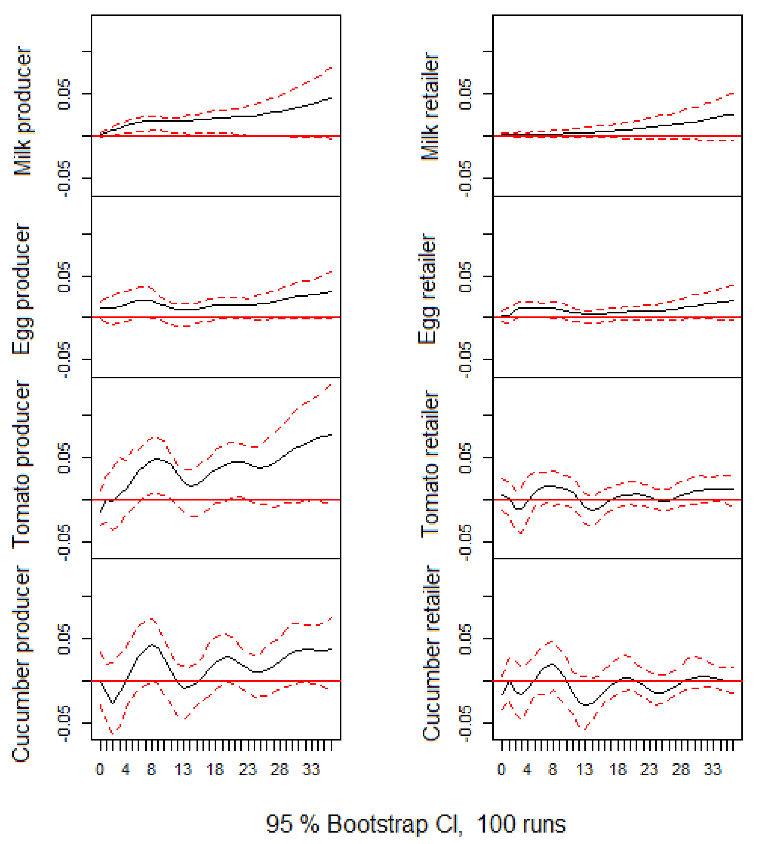
5.3. Impulse Response Function

The impulse response function is adopted to reflect the changes in a given variable that occurred after an exterior shock. The function designates the rate at which an unforeseen variation in the impulse variable influences the response variable during a particular period of time. Figure 3 shows the reaction of producer and retail prices of the agricultural commodities investigated to diesel price. For this analysis, we used a period of thirty-six months, long enough to explain any significant price response. Furthermore, there are investigations on the conduct of commodity prices that establish that they behave variously amongst crisis periods [94]. In this study, the impulse response analysis uses the economic crisis period and depicts the related curves of the impulse response. We used the period between March 2020 and July 2022 as the crisis period encompassing both the COVID-19 pandemic of 2020 and the Russia–Ukraine war of 2022.

The functions of impulse response illustrate that producer prices in the cow’s milk and chicken egg markets react positively to the price of diesel over the whole thirty-sixth month period. Regarding cow’s milk producer prices, an initial increase in price up to the sixth month is followed by price stabilization until the fifteenth month, and a constant increase in price after this period is observed. As for cow’s milk retail prices, the eventual response nears zero in the first ten months, and the response constantly grows after this period. The producer chicken egg price initially stabilizes until the third month and after this, the price rises, stabilizes, decreases and stabilizes again until the seventeenth month. The price constantly increases after this period. A similar development is observed with the retail egg price, with the difference that the eventual response is closer to zero throughout the thirty-six-month period, and the second stabilization period is a longer one (from the second to the eighth month).

Although it starts with a negative change in the producer price of greenhouse tomatoes caused by diesel price, the response turns out to be positive after the third month, followed by a successive increase and decrease until the twenty-sixth month, with a constant rise in prices after this period. Retail prices of greenhouse tomatoes respond initially positively to diesel prices, with the response becoming negative from the third to the fifth month. This successive alternation of positive and negative price response alternates until the thirty-first month, and the response becomes constant after this period.

Regarding greenhouse cucumbers, the initial response is negative over the first four months, and the response becomes positive for the next eight months. Producer and retail prices respond negatively during the next period covering four and eight months, respectively. Producer prices become only positive after the fifteenth month, while retail prices respond successively in a positive and negative manner until the end of the thirty-sixth month.

It is indicated by the impulse response function results that the prices of agricultural commodities respond to diesel price shocks, an ascertainment that confirms the decision obtained by the results of the Granger causality test. From the fact that the diesel price shows episodes of great alterations as depicted in Figure 1, this decision illustrates that the answer of agricultural commodity prices is proportional to diesel price changes. Bearing in mind that the analysis encompassed periods covering the financial crisis in Bulgaria produced by the COVID-19 pandemic and the Russia–Ukraine war, the fact that diesel prices did change significantly after November 2020 shows that the reaction of agricultural commodities prices was immense.

6. Conclusions

It was demonstrated by the results of the investigation that the size and direction of commodity price handover along the agricultural commodity supply chain are based on the commodity type and whether the considered period involves the short run or the long run. The result of the Granger causality short-run test has displayed a significant two-way connection only in the greenhouse tomato and cucumber markets. The producer prices of these two types of vegetable markets have a greater effect than the price of retail, a clear sign that producers are more capable of handing over prices to retailers than the opposite. Juxtaposing this result with the long-run elasticity results of the VECM, it is noticed that the retail price of greenhouse tomatoes converges to equilibrium, while producer prices diverge. The producer price of greenhouse cucumbers converges to equilibrium, and the retail price differs. As for the cow’s milk and chicken egg markets, even though producer prices impacted retail prices in the short run, there is no long-run rapprochement.

The results of the connection between diesel and agricultural commodity prices also expose contrasts in the kind of market price. It is observed from the Granger causality test results that variation in diesel prices drastically affects retail prices in the chicken egg and greenhouse cucumber markets, but it has an effect on producer prices only in the cow’s milk market. The direction for all these impacts is positive, showing that a rise in the price of diesel causes an increase in agricultural commodity prices.

It is essential to note that the differences in producer prices of chicken eggs and greenhouse cucumbers lead to a considerable increase in retail prices. Therefore, the impact of producer prices is higher than that of diesel prices. This result corroborates the speculations of market force and profits. By rising profits, retailers in chicken egg and greenhouse cucumber markets resort to selling more eggs and cucumbers. However, this also reduces their capability to raise egg and cucumber prices when their producer prices increase.

As a final note, this article presents a complete investigation of the relationship between diesel, producer and retail prices of four agricultural commodities (cow’s milk, chicken eggs, greenhouse tomatoes and cucumbers). Based on this fact, the obtained results have useful inferences for producers, retail, and policy makers. The connections of prices depicted that these five markets permit policy makers to evolve particular policies and merchants to forecast tendencies in the studied agricultural commodity prices. Government subsidies in modern countries have often aimed at farmers, with the aim to help them obtain higher incomes [68]. The study has confirmed the fact that in the event of a diesel price shock, the effectiveness of such approaches at improving the well-being of producers is particular to the market in which these schemes are put into practice. In definite markets (such as the chicken egg and greenhouse cucumber markets), the producer price impact is greater than the diesel price impact. On such occasions, policy improvements during diesel price variations are required to decrease the impact of the discrepancy between retail and producer prices.

There are some limitations related to this study that should be covered by future research. To start with, the use of national data in this study means that it is not possible to distinguish between the prices of agricultural commodity markets in the different regions of Bulgaria from the prices of agricultural commodity markets on a national level. A future study could use data for agricultural commodity prices for the six regions of Bulgaria: the north-west region, north-central region, north-east region, south-west region, south-central region and south-east region.

A second weakness is that this study used data for agricultural commodities that are highly perishable. A future study can include data on durable agricultural commodities.

References

1. Ozili, P.K.; Arun, T. Spillover of COVID-19: Impact on the Global Economy. Available online: https://papers.ssrn.com/sol3/papers.cfm?abstract_id=3562570 (accessed on 20 May 2022).
2. World Economic Outlook. April 2022. Available online: https://www.imf.org/en/Publications/WEO/Issues/2022/04/19/world-economic-outlook-april-2022 (accessed on 21 May 2022).
3. Extra EU Imports of Petroleum Oil from Main Trading Partners, 2020 and First Semester 2021. Available online: https://ec.europa.eu/eurostat/statistics-explained/index.php?title=File:Extra_EU_imports_of_petroleum_oil_from_main_trading_partners,_2020_and_first_semester_2021.png (accessed on 21 May 2022).
4. NPR: The EU just Proposed a Ban on Oil from Russia, Its Main Energy Supplier. Available online: https://www.npr.org/2022/05/04/1096596286/eu-europea-russia-oil-ban (accessed on 30 April 2022).
5. Reuters: Bulgaria to Seek Exemption from EU Oil Embargo on Russia if Possible, Deputy PM Says. Available online: https://www.reuters.com/business/energy/bulgaria-seek-exemption-any-eu-embargo-russian-oil-deputy-pm-says-2022-05-04/ (accessed on 4 May 2022).
6. Ganev, E.I.; Ivanov, B.B.; Dobrudzhaliev, D.G.; Dzhelil, Y.R.; Nikolova, D. Adopting environmental transportation practice in biodisel production as key factor for sustainable development: A Bulgarian case study. Bulg. Chem. Commun. 2018, 50, 106–111. [Google Scholar]
7. Prakash, A. Why volatility matters. In Safeguarding FoodSecurity in Volatile Global Markets; Prakash, A., Ed.; FAO: Rome, Italy, 2011; pp. 1–24. [Google Scholar]
8. Rapsomanikis, G.; Hallam, D. Threshold Cointegration in the Sugar–Ethanol–Oil Price System in Brazil: Evidence from Nonlinear Vector Error Correction Models; FAO: Rome, Italy, 2006; pp. 1–20. [Google Scholar]
9. Min, H. Examining the impact of energy price volatility on commodity prices from energy supply chain perspectives. Energies 2022, 15, 7957. [Google Scholar] [CrossRef]
10. Raneses, A.R.; Glaser, L.K.; Price, J.M.; Duffield, J.A. Potential biodiesel markets and their economic effects on the agricultural sector of the United States. Ind. Crops Prod. 1999, 9, 151–162. [Google Scholar] [CrossRef]
11. Nazlioglu, S.; Soytas, U. World oil prices and agricultural commodity prices: Evidence from an emerging market. Energy Econ. 2011, 33, 488–496. [Google Scholar] [CrossRef]
12. Awan, A.G.; Imran, M. Factors affecting food price inflation in Pakistan. ABC J. Adv. Res. 2015, 4, 75–90. [Google Scholar] [CrossRef]
13. Coronado, S.; Rojas, O.; Romero-Meza, R.; Serletis, A.; Chiu, L.V. Crude Oil and Biofuel Agricultural commodity prices. In Uncertainty, Expectations and Asset Price Dynamics. Dynamic Modeling and Econometrics in Economics and Finance; Jawadi, F., Ed.; Springer: Cham, Switzerland, 2018; pp. 117–123. [Google Scholar]
14. Meyer, D.F.; Sanusi, K.A.; Hassan, A. Analysis of the asymmetric impacts of oil prices on food prices in oil-exporting developing countries. J. Int. Stud. 2018, 11, 82–94. [Google Scholar] [CrossRef] [PubMed]
15. Zafeiriou, E.; Arabatzis, G.; Karanikola, P.; Tampakis, S.; Tsiantikoudis, S. Agricultural commodities and crude oil prices: An empirical investigation of their relationship. Sustainability 2018, 10, 1199. [Google Scholar] [CrossRef] [Green Version]
16. Chengab, S.; Cao, Y. On the relation between global food and crude oil prices: An empirical investigation in a nonlinear framework. Energy Econ. 2019, 81, 422–432. [Google Scholar] [CrossRef]
17. Ngare, L.W.; Derek, O.W. The effect of fuel prices on food prices in Kenya. In Proceedings of the 6th African Conference of Agricultural Economists, Abuja, Nigeria, 23–26 September 2019. [Google Scholar]
18. Shiferaw, Y.A. Time-varying correlation between agricultural commodity and energy price dynamics with Bayesian multivariate DCC-GARCH models. Phys. A Stat. Mech. Appl. 2019, 526, 120807. [Google Scholar] [CrossRef]
19. Siami-Namini, S. Volatility transmission among oil price, exchange rate and agricultural commodities prices. AEF 2019, 6, 41–61. [Google Scholar] [CrossRef]
20. Barbaglia, L.; Croux, C.; Wilms, I. Volatility spillovers in commodity markets: A large t-vector autoregressive approach. Energy Econ. 2020, 85, 104555. [Google Scholar] [CrossRef]
21. Elleby, C.; Domínguez, I.P.; Adenauer, M.; Genovese, G. Impacts of the COVID-19 Pandemic on the Global Agricultural Markets. ERE 2020, 76, 1067–1079. [Google Scholar] [CrossRef] [PubMed]
22. Pronko, L.; Furman, I.; Kucher, A.; Gontaruk, Y. Formation of a state support program for agricultural producers in Ukraine considering world experience. Eur. J. Sustain. Dev. 2020, 9, 364–379. [Google Scholar] [CrossRef]
23. Aye, G.C.; Odhiambo, N.M. Oil prices and agricultural growth in South Africa: A threshold analysis. Resour. Policy 2021, 73, 102196. [Google Scholar] [CrossRef]
24. Chowdhury, M.A.F.; Meo, M.S.; Uddin, A.; Haque, M.M. Asymmetric effect of energy price on commodity price: New evidence from NARDL and time frequency wavelet approaches. Energy 2021, 231, 120934. [Google Scholar] [CrossRef]
25. Haddad, H.B.; Mezghani, I.; Gouider, A. The dynamic spillover effects of macroeconomic and financial uncertainty on commodity markets Uncertainties. Economies 2021, 9, 91. [Google Scholar] [CrossRef]
26. Kaulu, B. Effects of crude oil prices on copper and maize prices. Futur. Bus. J. 2021, 7, 54. [Google Scholar] [CrossRef]
27. Zimmer, Y.; Marque, G.V. Energy cost to produce and transport crops—The driver for crop prices? Case study for Mato Grosso, Brazil. Energy 2021, 225, 120260. [Google Scholar] [CrossRef]
28. Shahzada, U.; Jena, S.K.; Tiwaric, A.K.; Doğand, B.; Magazzino, C. Time-frequency analysis between Bloomberg Commodity Index (BCOM) and WTI crude oil prices. Resour. Policy 2022, 78, 102823. [Google Scholar] [CrossRef]
29. Umar, Z.; Gubareva, M.; Naeem, M.; Akhter, A. Return and volatility transmission between oil price shocks and agricultural commodities. PLoS ONE 2021, 16, e0246886. [Google Scholar] [CrossRef]
30. Esmaeili, A.; Shokoohi, Z. Assessing the effect of oil price on world food prices: Application of principal component analysis. Energy Policy 2011, 39, 1022–1025. [Google Scholar] [CrossRef]
31. Baumeister, C.; Kilian, L. Do oil price increases cause high. Econ. Policy. 2014, 29, 693–747. [Google Scholar] [CrossRef] [Green Version]
32. Wong, S.K.; Shamsudin, N.M. Impact of crude oil price, exchange rate and real GDP on Malaysia’s food price fluctuations: Symmetric or asymmetric? Int. J. Econ. Manage. 2017, 11, 259–273. [Google Scholar]
33. Abdlaziz, R.A.; Rahim, A.K.; Adamu, P. Oil and food prices co-integration nexus for Indonesia: A non-linear autoregressive distributed lag analysis. Int. J. Energy Econ. Policy 2016, 6, 82–87. [Google Scholar]
34. Nazlioglu, S. World oil and agricultural commodity prices: Evidence from nonlinear causality. Energy Policy 2011, 39, 2935–2943. [Google Scholar] [CrossRef]
35. Rosa, F.; Vasciaveo, M. Agri-commodity price dynamics: The relationship between oil and agricultural market. In Proceedings of the International Association of Agricultural Economists (IAAE) Triennial Conference, Foz do Iguaçu, Brazil, 18–24 August 2012. [Google Scholar]
36. Su, C.W.; Wang, X.Q.; Tao, R.; Oana-Ramona, L. Do oil prices drive agricultural commodity prices? Further evidence in a global bio-energy context. Energy 2019, 172, 691–701. [Google Scholar] [CrossRef]
37. Roman, M.; Górecka, A.; Domagała, J. The linkages between crude oil and food prices. Energies 2020, 13, 6545. [Google Scholar] [CrossRef]
38. Vo, D.H.; Vu, T.N.; Vo, A.T.; McAleer, M. Modeling the relationship between crude oil and agricultural commodity prices. Energies 2019, 12, 1344. [Google Scholar] [CrossRef] [Green Version]
39. Pal, D.; Mitra, S.K. Correlation dynamics of crude oil with agricultural commodities: A comparison between energy and food crops. Econ. Model. 2019, 82, 453–466. [Google Scholar] [CrossRef]
40. Ji, Q.; Bouri, E.; Roubaud, D.; Shahzad, S.J.H. Risk spillover between energy and agricultural commodity markets: A dependence-switching CoVaR-copula model. Energy Econ. 2018, 75, 14–27. [Google Scholar] [CrossRef]
41. Pasrun, A.; Rosnawintang, R.; Saidi, L.D.; Tondi, L.; Sani, L.O.A. The causal relationship between crude oil price, exchange rate and rice price. Int. J. Energy Econ. Policy 2018, 8, 90–94. [Google Scholar]
42. Al-Maadid, A.; Caporale, G.M.; Spagnolo, F.; Spagnolo, N. Spillovers between food and energy prices and structural breaks. Int. Econ. 2017, 150, 1–18. [Google Scholar] [CrossRef]
43. Bergmann, D.; O’Connor, D.; Thummel, A. An analysis of price and volatility transmission in butter, palm oil and crude oil markets. Agric. Food Econ. 2016, 4, 23. [Google Scholar] [CrossRef] [Green Version]
44. Mawejje, J. Food prices, energy and climate shocks in Uganda. Agric. Food Econ. 2016, 4, 4. [Google Scholar] [CrossRef]
45. McFarlane, L. Agricultural commodity prices and oil prices: Mutual causation. Outlook Agric. 2016, 45, 87–93. [Google Scholar] [CrossRef] [Green Version]
46. Cabrera, B.L.; Schulz, F. Volatility linkages between energy and agricultural commodity prices. Energy Econ. 2016, 54, 190–203. [Google Scholar] [CrossRef] [Green Version]
47. Fernandez-Perez, A.; Frijns, B.; Tourani-Rad, A. Contemporaneous interactions among fuel, biofuel and agricultural commodities. Energy Econ. 2016, 58, 1–10. [Google Scholar] [CrossRef]
48. Hamulczuk, M. Energy prices vs agri-food prices—Energy security and food security. Humanit. Soc. Sci. 2016, 23, 37–51. [Google Scholar]
49. Ekeinde, E.B.; Dosunmu, A.; Okujagu, D.C.; Obazeh, D.J. Deregulation of the downstream sector of the Nigerian oil industry and its impact on pump price of petroleum products. In Proceedings of the SPE Nigeria Annual International Conference and Exhibition, Lagos, Nigeria, 3 August 2022. [Google Scholar]
50. Nwoko, I.C.; Aye, G.C.; Asogwa, B.C. Effect of oil price on Nigeria’s food price volatility. Cogent Food Agric. 2016, 2, 1146057. [Google Scholar]
51. Olujobi, O.J.; Olarinde, E.S.; Yebisi, T.E.; Okorie, U.E. COVID-19 pandemic: The impacts of crude oil price shock on Nigeria’s economy, legal and policy options. Sustainability 2022, 14, 11166. [Google Scholar] [CrossRef]
52. Zhang, C.; Qu, X. The effect of global oil price shocks on China’s agricultural commodities. Energy Econ. 2015, 51, 354–364. [Google Scholar] [CrossRef]
53. Koirala, K.H.; Mishra, A.K.; D’Antoni, J.M.; Mehlhorn, J.E. Energy prices and agricultural commodity prices: Testing correlation using copulas method. Energy 2015, 81, 430–436. [Google Scholar] [CrossRef]
54. Rezitis, A.N. The relationship between agricultural commodity prices, crude oil prices and US dollar exchange rates: A panel VAR approach and causality analysis. Int. Rev. Appl. Econ. 2015, 29, 403–434. [Google Scholar] [CrossRef]
55. Chang, T.-H.; Su, H.-M. The substitutive effect of biofuels on fossil fuels in the lower and higher crude oil price periods. Energy 2010, 35, 2807–2813. [Google Scholar] [CrossRef]
56. Sahara, A.D.; Amaliah, S.; Irawan, T.; Dilla, S. Economic impacts of biodiesel policy in Indonesia: A computable general equilibrium approach. J. Econ. Struct. 2022, 11, 22. [Google Scholar] [CrossRef]
57. Campiche, J.L.; Bryant, H.L.; Richardson, J.W.; Outlaw, J.L. Examining the Evolving Correspondence Between Petroleum Prices and Agricultural Commodity Prices. In Proceedings of the American Agricultural Economics Association, Portland, OR, USA, 29 July–1 August 2007. [Google Scholar]
58. Bekiros, S.D.; Diks, C.G. The relationship between crude oil spot and futures prices: Cointegration, linear and nonlinear causality. Energy Econ. 2008, 30, 2673–2685. [Google Scholar] [CrossRef]
59. Saghaian, S.H. The impact of the oil sector on commodity prices: Correlation or causation? J. Agric. Appl. Econ. 2010, 42, 477–485. [Google Scholar] [CrossRef] [Green Version]
60. Natanelov, V.; Alam, M.J.; McKenzie, A.M.; Huylenbroeck, G.V. Is there co-movement of agricultural commodities futures prices and crude oil? Energy Policy 2011, 39, 4971–4984. [Google Scholar] [CrossRef] [Green Version]
61. Rajeaniova, M.; Pokriveak, J. The impact of biofuel policies on food prices in the European Union. Ekon. Cas. 2011, 59, 459–471. [Google Scholar]
62. Ziegelback, M.; Kastner, G. European rapeseed and fossil diesel: Threshold cointegration analysis and possible implications. In Proceedings of the Name of the 51st Annual Meeting of Gewisola, Corporative Agriculture: Between Market Needs and Social Expectations, Halle, Germany, 28–30 September 2011. [Google Scholar]
63. Nazlioglu, S.; Soytas, U. Oil price, agricultural commodity prices, and the dollar: A panel cointegration and causality analysis. Energy Econ. 2012, 34, 1098–1104. [Google Scholar] [CrossRef]
64. Natanelov, V.; McKenzie, A.M.; Huylenbroeck, G.V. Crude oil–corn–ethanol–nexus: A contextual approach. Energy Policy 2013, 63, 504–513. [Google Scholar] [CrossRef]
65. David, S.A.; Inácio, C.M.C.; Machado, J.A.T. Ethanol Prices and Agricultural Commodities: An Investigation of Their Relationship. Mathematics 2019, 7, 774. [Google Scholar] [CrossRef] [Green Version]
66. Zingbagba, M.; Nunes, R.; Fadairo, M. The impact of diesel price on upstream and downstream food prices: Evidence from São Paulo. Energy Econ. 2020, 85, 104531. [Google Scholar] [CrossRef]
67. Sexton, J.R. Market power, misconceptions, and modern agricultural markets. Am. J. Agric. Econ. 2012, 95, 209–219. [Google Scholar] [CrossRef]
68. McCorriston, S.; Morgan, C.W.; Rayner, A.J. Price transmission: The interaction between market power and returns to scale. Eur. Rev. Agric. Econ. 2001, 28, 143–159. [Google Scholar] [CrossRef]
69. Meyer, J.; von Cramon-Taubadel, S. Asymmetric price transmission: A survey. J. Agric. Econ. 2004, 55, 581–611. [Google Scholar] [CrossRef] [Green Version]
70. Fuelo. Available online: https://bg.fuelo.net/ (accessed on 30 July 2022).
71. Bowman, K.; Shenton, L. Omnibus test contours for departures from normality based on b1 and b2. Biometrika 1975, 62, 243–250. [Google Scholar] [CrossRef]
72. Thadewald, T.; Büning, H. Jarque-Bera test and its competitors for testing normality: A power comparison. J. Appl. Stat. 2007, 34, 87–105. [Google Scholar] [CrossRef]
73. Greene, W.H. Econometric Analysis, 3rd ed.; Macmillan Publishing Company: New York, NY, USA, 1997. [Google Scholar]
74. Akaike, H. A new look at the statistical model identification. IEEE Trans. Automat. Contr. 1974, 19, 716–723. [Google Scholar] [CrossRef]
75. Burnham, K.P.; Anderson, D.R. Model Selection and Multimodel Inference: A Practical Information-Theoretic Approach, 2nd ed.; Springer: New York, NY, USA, 2002. [Google Scholar]
76. Claeskens, G.; Hjort, N.L. Model Selection and Model Averaging, 1st ed.; Cambridge University Press: Cambridge, UK, 2008. [Google Scholar]
77. Wit, E.; Edwin van den, H.; Jan-Willem, R. ’All models are wrong…’: An introduction to model uncertainty. Stat. Neerl. 2012, 66, 217–236. [Google Scholar] [CrossRef] [Green Version]
78. Johansen, S.; Juselius, K. Maximum likelihood estimation and inference on cointegration: With applications to the demand for money. Oxf. Bull. Econ. Stat. 1990, 52, 169–210. [Google Scholar] [CrossRef]
79. Johansen, S. Estimation and hypothesis testing of cointegration vectors in Gaussian vector autoregressive models. Econometrica 1991, 59, 1551–1580. [Google Scholar] [CrossRef]
80. Brooks, C. Introductory Econometrics for Finance, 2nd ed.; Cambridge University Press: New York, NY, USA, 2008. [Google Scholar]
81. Engle, R.; Granger, C. Co-integrationand error correction: Representation, estimation, and testing. Econometrica 1987, 35, 251–276. [Google Scholar] [CrossRef]
82. Lakshmanasamy, T. Inflation and Macroeconomic Performance in India: Vector Error Correction Model Estimation of the Causal Effects. JQFE 2022, 4, 17–37. [Google Scholar]
83. Jarque, C.M.; Bera, A.K. A Test for Normality of Observations and Regression Residuals. Int. Stat. Rev. 1987, 55, 163–172. [Google Scholar] [CrossRef]
84. Brufatto, V. Macroeconomic Factors and the U.S. Stock Market Index: A Cointegration Analysis; Ca’Foscari University of Venice: Venice, Italy, 2016. [Google Scholar]
85. Engle, R.F. Autoregressive Conditional Heteroscedasticity with Estimates of the Variance of United Kingdom Inflation. Econometrica 1982, 50, 987–1007. [Google Scholar] [CrossRef]
86. Lütkepohl, H.; Krätzig, M. Applied Time Series Econometrics, 1st ed.; Cambridge University Press: New York, NY, USA, 2004. [Google Scholar]
87. Box, G.E.P.; Pierce, D.A. Distribution of the Residual Autocorrelations in Autoregressive-Integrated Moving-Average Time Series Models. J. Am. Stat. Assoc. 1970, 65, 1509–1526. [Google Scholar] [CrossRef]
88. Ljung, G.M.; Box, G.E.P. On a Measure of a Lack of Fit in Time Series Models. Biometrika 1978, 65, 297–303. [Google Scholar] [CrossRef]
89. Nikolov, N. Transport and transport security. Mech. Transp. Commun. 2012, 10, 66–73. (In Bulgarian) [Google Scholar]
90. Dimitrov, G. Trends in the development of land freight transport in Bulgaria. Sci. Pap. UNWE 2021, 1, 49–83. (In Bulgarian) [Google Scholar]
91. Hair, J.; Black, W.C.; Babin, B.J.; Anderson, R.E. Multivariate Data Analysis, 7th ed.; Pearson: Upper Saddle River, NJ, USA, 2010. [Google Scholar]
92. Byrne, B.M. Structural Equation Modeling with AMOS: Basic Concepts, Applications, and Programming, 3rd ed.; Routledge: New York, NY, USA, 2016. [Google Scholar]
93. Gupta, D.; Kamilla, U. Dynamic Linkages between Implied Volatility Indices of Developed and Emerging Financial Markets: An Econometric Approach. Glob. Bus. Rev. 2015, 16, 46–57. [Google Scholar] [CrossRef]
94. Esposti, R.; Listorti, G. Agricultural price transmission across space and commodities during price bubbles. In Proceedings of the EAAE 2011 Congress, Zurich, Switzerland, 30 August–2 September 2011. [Google Scholar]
Figure 1. Monthly diesel price from January 2011 to July 2022.
Mathematics 11 00559 g001
Figure 2. Monthly prices of cow’s milk, chicken eggs, greenhouse tomatoes and greenhouse cucumbers from January 2011 to July 2022.
Mathematics 11 00559 g002
Figure 3. Orthogonal impulse response of agricultural commodity prices to diesel price.
Mathematics 11 00559 g003