Queueing System with Potential for Recruiting Secondary Servers

Abstract

In this paper, we consider a single server queueing system in which the arrivals occur according to a Markovian arrival process (MAP). The served customers may be recruited (or opted from those customers’ point of view) to act as secondary servers to provide services to the waiting customers. Such customers who are recruited to be servers are referred to as secondary servers. The service times of the main as well as that of the secondary servers are assumed to be exponentially distributed possibly with different parameters. Assuming that at most there can only be one secondary server at any given time and that the secondary server will leave after serving its assigned group of customers, the model is studied as a QBD-type queue. However, one can also study this model as a GI/M/1-type queue. The model is analyzed in steady state, and a few illustrative numerical examples are presented.

1. Introduction

Queueing theory has been playing a significant role in many areas of science, engineering, and business, among others. One can see the impact of queueing theory in day-to-day activities. Starting from conventional applications in areas such as the telephone industry, grocery stores, post offices, and banks, queueing theory has permeated deep into emerging areas, including crowdsourcing and blockchains. In these emerging areas, businesses as well as other service sectors always look for ways to increase their efficiency by recruiting (temporary) servers who can help the system when needed.

In this paper, we introduce a new queueing model where the system will try to recruit secondary servers from among the customers who received services and are willing to serve. The motivation for studying such a queueing system arose out of one of the author’s personal experiences visiting a bank. In countries like India, government pensioners are required to send a living proof document once a year to the government via banks. During one such visit with an aging parent, the author had to wait for a long period of time before a bank agent helped his parent obtain a simple one-page document to be filled out and signed by the parent; then, the completed document was stamped by the agent. The meeting with the agent took fewer than a couple of minutes, but the aging parent could have saved time and could have been spared the agony of waiting if only they had a secondary server available to help the agent with such services. Similar examples can be seen in areas where customers who are required to use computers for filling out necessary forms are not comfortable with computers; they may benefit from having such a secondary server facility. In order to recruit such secondary servers, the customers need to know the requirements to go through such a process. In education applications, students or teaching assistants (who keep rotating based on the quarter/system) or any other form of helpers can, after getting serviced by the teacher, be recruited temporarily to help the system. In sports, the training manager can, after training athletes, be recruited to help the team. In computer applications, especially dealing with multi-core CPUs, a few can be programmed (similar to recruitment) to help the system. Secondly, there should be a willingness on the part of the customers to help other customers.

Thus, the novelty of this paper is to introduce the concept of recruitment of secondary servers from the (served) customers so as to help the system. Further, these secondary servers will offer services in groups of varying sizes and are available only on a temporary basis (will leave the system after serving exactly one group). In this way, the customers will not be held back so as to attend to their business after helping the system. The numerical results indicate the proposed model performs better than the corresponding classical queueing model. This will help the decision maker of the system recruit secondary servers as and when needed in order to improve the performance of the system.

Queueing models where the main servers are supported by backup servers (or additional servers) are interesting from a practical point of view. For example, one can find the usefulness of such backup server queueing models in energy saving applications in cloud computing systems and server farms (see, e.g., the survey paper [1] and the paper [2]). Queueing models with reserve servers studied in the literature are divided into two groups. One group, seemingly a larger one, assumes a switching-on and a switching-off mechanism for the backup servers based on the current queue length using threshold-type and hysteresis-type strategies. It is worth mentioning a few works from this group, namely, papers [3,4,5,6,7,8,9,10,11,12,13,14,15,16,17,18,19,20,21,22].

In the other group of papers, the focus is on using backup servers to help the main server whenever there is too long a service duration for the customer in service. In [23], a multi-server queueing model with phase-type services is considered. If the service time of a customer exceeds a certain (random) bound, the server will start receiving help from a backup server from a finite pool of backup servers. Also, a few practical examples dealing with managerial decision are presented. In [24], a multi-server infinite buffer queueing system with additional servers (assistants) provides help to the main servers whenever the server encounters problems that are commonly noticed in real-world situations.

In this paper, we consider a model in which the arrivals occur according to the Markovian arrival process ($MAP$). Recall that $MAP$, a class of versatile point processes, was introduced by Neuts in the 1970s. For details on $MAP$ and its usefulness in stochastic modeling, we refer the reader to [25,26,27,28,29,30,31,32,33,34,35,36,37,38,39,40]. Among the papers considering systems with $MAP$ and backup servers, we point out a few relevant ones here.

In [41], a multi-server queueing model of the type $MAP/M/c$—in which a permanent server is supported by a group backup servers that are added or removed based on a set of thresholds dynamically—is considered, and some interesting results useful in practical applications are reported. In [42], under the scenario of a finite capacity queueing system with phase-type services, the main server is supported by a backup server based on a hysteretic-type threshold. That is, a backup server is requested (the request time is assumed to be exponential) when the buffer size hits the upper threshold, and this server is released whenever the buffer size drops to or below the lower threshold at the service completion of the backup server. Through numerical examples, they study the impact of the standard deviation as well as the correlation of the inter-arrival times and the standard deviation of the service time distributions on the server backup decisions. A $MAP/PH/1$ queueing model is studied in [43] using a simulation approach wherein, using a set of thresholds, the backup servers are added through requests taking a random amount of time and released. A queueing model with phase-type services wherein the server is subject to breakdowns and repairs is considered in [44] by taking into consideration a backup server only during periods of downtime.

In [45], the authors study a model in which two types of customers arrive according to a marked Markovian arrival process ($MMAP$) such that the type that receives anon-preemptive priority has a finite buffer, and the other type has an infinite buffer to wait, and in which the services are of the phase type depending on the type. Multiple servers are always active, while some are switched on and off depending a hysteretic policy. The main contribution of the paper is the development of a computational procedure for the stationary distribution of the system states and optimal cost criterion for any fixed threshold. The authors show through numerical results the effectiveness of the hysteresis control and the importance of the role played by the correlation in the arrival process as well as the variance of the service times.

In this paper, using $MAP$ as an arrival process, we consider a scenario of providing help to the main server in a single-server queueing system. This scenario was considered earlier in the context of crowdsourcing [46]. Crowdsourcing is getting popular after a number of industries such as food, consumer products, hotels, electronics, and other large retailers bought into this idea of serving customers; see, e.g., [47,48,49,50]. In [46], a multi-server queue was considered in which there are two types of customers. One type of customers, after obtaining a service, may opt to help the system by acting as a secondary server and hence decrease the number waiting in the system by one. In this paper, we consider the system that is also suitable for modeling the crowdsourcing system. In contrast to [46], here we assume that there is only one main server and that the use of only one secondary server is allowed at any give time. However, we consider the two following features that are inherent to some real world systems and have not been studied in the past: (i) a secondary server will be assigned a batch (not exceeding a pre-determined finite threshold); this server will offer services one at a time; and once all the assigned customers are served, the secondary server also leaves the system; and (ii) with a certain probability, a customer served by a secondary server becomes dissatisfied and hence returns to the main system to get a new service.

The paper is organized as follows. In Section 2, the description of the mathematical model is presented. The steady state analysis using the $QBD$-type process of the model is given in Section 3, and the $GI/M/1$-type approach is presented in Section 4. Illustrative numerical examples are given in Section 5, and a few concluding remarks are summarized in Section 6.

2. Mathematical Model

We consider a single-server queueing system in which the arrivals occur according to a Markovian arrival process ($MAP$) with parameter matrices $(D_0,D_1)$ of order $m.$ The $MAP$, introduced first by Neuts [36] as part of a larger class of point processes referred to as versatile Markovian point process with heavy notation, was reintroduced in paper [34] with simpler notation. The simplicity of the notation has attracted many researchers, and hence this representation is now the standard in the literature when using $MAP$ or batch $MAP$ ($BMAP$). The $MAP$ generalizes some of the well-known point processes like Poisson, interrupted Poisson, and phase-type renewals, among others. Further, $MAP$ is ideally suited in situations where correlation maybe present in the inter-arrival times. Suppose that the arrivals occur from different sources to a common area for processing. Even if all the individual sources generate arrivals according to renewal processes, the pooled one may not necessarily be a renewal process (unless all individual sources are Poisson processes). Another attractive part of using $MAP$ is that the analysis requires matrix formalism and the associated intuitive reasonings that go with the analysis. A quick description of the $MAP$ follows; for more details, we refer the reader to the above references. The irreducible generator of the $MAP$ is given by $D_0+D_1$; let $\mathit{\delta }$ denote its invariant vector so that

$$\mathit{\delta }(D_0+D_1)=0,\mathit{\delta }\mathit{e}=1,$$

(1)

where here and in the following, e denotes a column vector of ones with appropriate dimension and 0 denotes a row vector of zeros with appropriate dimension.

While the matrix $D_0$ governs the transitions corresponding to the underlying generator producing no arrivals, the matrix $D_1$ governs those corresponding to arrivals occurring to the system.

The average rate of the arrivals ($\lambda$), the variance of the inter-arrival times (${\sigma }^2$), and the correlation (${\rho }_c$) between two successive inter-arrival times are given by (see, e.g., ref. [29])

$$\begin{array}{c}\lambda =\mathit{\delta }{D}_1\mathit{e},{\sigma }^2=\frac{2}{\lambda }\mathit{\delta }{(-D_0)}^{-1}\mathit{e}-\frac{1}{{\lambda }^2},\\ \\ {\rho }_c=\frac{\lambda \mathit{\delta }{(-D_0)}^{-1}{D}_1{(-D_0)}^{-1}\mathit{e}-1}{2\lambda \mathit{\delta }{(-D_0)}^{-1}\mathit{e}-1}.\end{array}$$

(2)

The system has a single server that offers services on a $FCFS$ basis. This server will be referred to as the main server. The service times are exponential with the parameter ${\mathit{\mu }}_1$.

With probability $p,0\le p\le 1$, a served customer may be recruited (or opted from the served customer point of view) to serve other customers waiting in the system (assuming the queue size is positive) provided there is no other such server already serving. Such a server is referred to as a secondary server. That is, a recruitment occurs only when there is at least one customer waiting in the queue and when there is no other secondary server present in the system. Thus, the system may have at most two servers at any given time. Note that with probability $q=1-p$, the served customer, who can become the secondary server, does not agree to do this and leaves the system.

When a secondary server is recruited, the server will be assigned a group of, say, i customers, where $i=min\{$number in the queue, $L\}$, where L is a pre-determined finite positive integer. That is, $1\le L<\infty$. The secondary server will offer services to the group of customers one at a time, and the service times are exponentially distributed with parameter ${\mathit{\mu }}_2$. A customer receiving a service from a secondary server may be dissatisfied with the service received and requests to be served again with probability $\nu ,0\le \nu \le 1$, and with probability $\tilde{\nu }=1-\nu$ will leave the system. The dissatisfied customers are fed back to the system. Once the secondary server finishes serving all the customers assigned, the system will release this server.

Note that by taking $p=0$ (in this case $\nu$ plays no role and can be ignored), we get the classic single-server queueing model. This case is used only as an accuracy check in the numerical computations and is not of interest otherwise. The case when $\nu =1$ is of no interest since here every customer served by a secondary server is fed back to the system and hiring secondary servers only makes the system slow down in offering services.

A pictorial description of the queueing system under study is displayed in Figure 1.

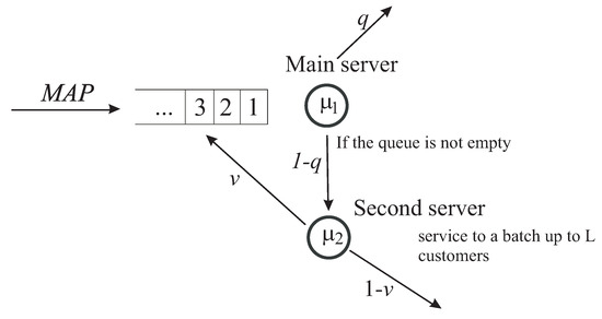
Figure 1. Structure of the system under study.

3. $QBD$ Approach to the Steady State Analysis

We will analyze the queueing model under study in steady state. The analysis can be carried out either via the $QBD$ process or via $GI/M/1$-type. In this section, we will take the $QBD$ approach, and in the next section, we briefly highlight the other approach. As it is known, the $QBD$ process is a special case of continuous-time Markov chain ($CTMC$). $QBD$ processes in the context of stochastic modeling have been extensively studied in the literature (see, e.g., refs. [26,29,30,31,32,33,37]).

3.1. Description of the $QBD$ Process Governing the System and Its Generator

Suppose that we denote, at time $t,t\ge 0$, that

•

$i_t$ is the number of customers in the system, $i_t\ge 0;$

•

$n_t$ is the number of customers in service at the secondary server, $n_t\in \{0,\cdots ,\min \{i_t,L\}\}$; (note that when $n_t=0$, the system does not have a secondary server);

•

${\xi }_t$ is the state of the underlying process of the $MAP$ describing the arrivals of the customers, ${\xi }_t=1,\cdots ,m.$

Then, the stochastic process, $\{{\zeta }_t=\{i_t,n_t,{\xi }_t\},t\ge 0\},$ describing the behavior of the model under study is a regular irreducible $CTMC$. Enumerating the states of the $CTMC$, $\{{\zeta }_t,t\ge 0\},$ in lexicographic order and denoting the level i, for $i\ge 0$, to be the set of states $\left\{\right(i,n,k):0\le n\le \min \{i,L\left\}\right\},1\le k\le m\}$, the (infinitesimal) generator, Q, of this $CTMC$ is given in the following theorem.

Theorem 1.

The infinitesimal generator Q of the $CTMC$$\{{\zeta }_t,t\ge 0\},$ has a block tri-diagonal structure:

$$Q=\left(\begin{array}{ccccccccccc}{Q}_{0,0}& Q_{0,1}& O& O& \dots & O& O& O& O& O& \dots \\ Q_{1,0}& Q_{1,1}& Q_{1,2}& O& \dots & O& O& O& O& O& \dots \\ O& Q_{2,1}& Q_{2,2}& Q_{2,3}& \dots & O& O& O& O& O& \dots \\ ⋮& ⋮& ⋮& ⋮& \ddots & ⋮& ⋮& ⋮& ⋮& ⋮& \ddots \\ O& O& O& O& \dots & Q_{L,L-1}& Q_{L,L}& Q^{+}& O& O& \dots \\ O& O& O& O& \dots & O& Q^{-}& Q^0& Q^{+}& O& \dots \\ O& O& O& O& \dots & O& O& Q^{-}& Q^0& Q^{+}& \dots \\ ⋮& ⋮& ⋮& ⋮& \ddots & ⋮& ⋮& ⋮& ⋮& ⋮& \ddots \end{array}\right),$$

(3)

where the non-zero blocks $Q_{i,j},$ are defined as follows:

$$\begin{array}{c}{Q}_{0,0}=D_0,\\ \\ Q_{i,i}=I_{i+1}\otimes D_0+\nu {\mathit{\mu }}_2{E}_i^{-}\otimes I_m-({\mathit{\mu }}_1{\widehat{I}}_i+{\mathit{\mu }}_2(I_{i+1}-{\overline{I}}_i))\otimes I_m,1\le i\le L,\\ \\ Q_{i,i}=Q^0=I_{L+1}\otimes D_0+\nu {\mathit{\mu }}_2{E}_L^{-}\otimes I_m-({\mathit{\mu }}_1{I}_{L+1}+{\mathit{\mu }}_2(I_{L+1}-{\overline{I}}_L))\otimes I_m,i>L,\\ \\ Q_{i,i+1}=E_i^{+}\otimes D_1,0\le i\le L-1,\\ \\ Q_{i,i+1}=Q^{+}=I_{L+1}\otimes D_1,i\ge L,\\ \\ Q_{1,0}=(1-\nu ){\mathit{\mu }}_2{\tilde{E}}_1^{-}\otimes I_m+{\mathit{\mu }}_1{I}_1^{-}\otimes I_m,1\le i\le L,\\ \\ Q_{i,i-1}=(1-\nu ){\mathit{\mu }}_2{\tilde{E}}_i^{-}\otimes I_m+q{\mathit{\mu }}_1{I}_i^{-}\otimes I_m+(1-q){\mathit{\mu }}_1{I}_i^{+}\otimes I_m,1\le i\le L,\\ \\ Q_{i,i-1}=Q^{-}=(1-v){\mathit{\mu }}_2{E}_L^{-}\otimes I_m+q{\mathit{\mu }}_1{I}_{(L+1)m}+(1-q){\mathit{\mu }}_1{I}^{+}\otimes I_m,i>L.\end{array}$$

(4)

In Equation (4), the notation used is as follows:

•

O and I are, respectively, zero and identity matrices of appropriate dimensions as indicated in the suffix;

•

⊗ indicates the Kronecker product of matrices (see, e.g., [51,52,53,54]);

•

$E_l^{+}$ is a matrix of dimension $(l+1)\times (l+2)$ with ${\left(E_l^{+}\right)}_{k,k}=1,0\le k\le l,$ and all other entries are zero;

•

$E_l^{-}$ is a square matrix of dimension $l+1$ with ${\left(E_l^{-}\right)}_{k,k-1}=1,1\le k\le l,$ and all other entries are zero;

•

${\widehat{I}}_l$ is a square matrix of dimension $l+1$ with ${\left({\widehat{I}}_l\right)}_{k,k}=1,0\le k\le l-1,$ and all other entries are zero;

•

${\overline{I}}_l$ is a square matrix of dimension $l+1$ with ${\left({\overline{I}}_l\right)}_{0,0}=1$, and all other entries are zero;

•

${\tilde{E}}_l^{-}$ is a matrix of dimension $(l+1)\times l$ with ${\left({\tilde{E}}_l^{-}\right)}_{k,k-1}=1,1\le k\le l,$ and all other entries are zero;

•

$I_l^{-}$ is the matrix of dimension $(l+1)\times l$ with ${\left(I_l^{-}\right)}_{k,k}=1,0\le k\le l-1,$ and all other entries are zero;

•

$I_l^{+}$ is the matrix of dimension $(l+1)\times l$ with ${\left(I_l^{+}\right)}_{0,l-1}=1,{\left(I_l^{+}\right)}_{k,k}=1,1\le k\le l-1,$ and all other entries are zero;

•

$I^{+}$ is the matrix of dimension $(L+1)\times (L+1)$ with ${\left(I^{+}\right)}_{k,k}=1,1\le k\le L,{\left(I^{+}\right)}_{0,L}=1,$ and all other entries are zero.

Proof. 

Follows immediately by considering various possibilities with respect to the transitions in the underlying $CTMC$. □

3.2. Ergodicity Condition of the $QBD$ Process

The following result establishes the stability condition of the queueing model under study.

Theorem 2.

The $CTMC$$\{{\zeta }_t,t\ge 0\}$ is ergodic if and only if the following inequality holds good:

$$\lambda <{\mathit{\mu }}_1+{\mathit{\mu }}_2(1-\nu )\frac{L(1-q){\mathit{\mu }}_1}{L(1-q){\mathit{\mu }}_1+{\mathit{\mu }}_2}.$$

(5)

Proof. 

It is well known from Neuts’ matrix-geometric approach (see, e.g., ref. [37]) that the criterion for the ergodicity of the $QBD$ with the generator of form given in (3) is the satisfaction of the inequality

$$\mathit{y}{Q}^{-}\mathit{e}>\mathit{y}{Q}^{+}\mathit{e},$$

(6)

where the vector y is the unique solution of the system

$$\mathit{y}(Q^{-}+Q^0+Q^{+})=\mathbf{0},\mathit{y}\mathit{e}=1.$$

(7)

It can easily be verified that

$$Q^{-}+Q^0+Q^{+}=I_{L+1}\otimes (D_0+D_1)+S\otimes I_m,$$

where

$$S=\left(\begin{array}{cccccc}-{\mathit{\mu }}_1(1-q)& 0& 0& \dots & 0& {\mathit{\mu }}_1(1-q)\\ {\mathit{\mu }}_2& -{\mathit{\mu }}_2& 0& \cdots & 0& 0\\ 0& {\mathit{\mu }}_2& -{\mathit{\mu }}_2& \dots & 0& 0\\ ⋮& ⋮& ⋮& \ddots & ⋮& ⋮\\ 0& 0& 0& \dots & {\mathit{\mu }}_2& -{\mathit{\mu }}_2\end{array}\right).$$

(8)

Using the mixed product rule for the Kronecker product of matrices (see, e.g., refs. [51,52]), and using Equation (1), it is easy to verify that

$$\mathit{y}=\mathit{x}\otimes \mathit{\delta },$$

(9)

where $\mathit{\delta }$ is as given in Equation (1) and x is the solution to the system

$$\mathit{x}S=\mathbf{0},\mathit{x}\mathit{e}=1.$$

(10)

By direct substitution, it is easy to verify that the components of the vector $\mathit{x}=(x_0,x_1,\cdots ,x_L),$ which is the unique solution to the system given in (10), are given by

$$x_0=\frac{{\mathit{\mu }}_2}{L(1-q){\mathit{\mu }}_1+{\mathit{\mu }}_2},x_i=\frac{{\mathit{\mu }}_1(1-q)}{L(1-q){\mathit{\mu }}_1+{\mathit{\mu }}_2},i=1,\cdots ,L.$$

(11)

The stated result follows from Equations (6), (9), and (11) along with the expression for $\lambda$ given in Equation (2). □

Remark 1.

The stability condition given in Equation (5) can intuitively be explained as follows. Generally, the ergodicity condition requires that the arrival rate of customers per unit of time should be less than the rate of services the customers receive per unit of time when the system is overloaded (in the sense that the number of customers presenting in the system is very large). Here, the arrival rate of the customers is λ per unit of time. The service rate of the customers when the system is overloaded is the sum of ${\mathit{\mu }}_1$ (the rate of service per unit of time by the main server) and the rate of service (per unit of time) provided by the secondary server. The latter service rate is 0 when the secondary server is not present at the system, which occurs with probability $x_0.$ When the secondary server is present in the system, which occurs with probability $(1-x_0)$, the customers receive service and leave the system at a rate ${\mathit{\mu }}_2(1-\nu )$ per unit of time. Thus, the total average service rate is ${\mathit{\mu }}_1+{\mathit{\mu }}_2(1-\nu )\frac{L(1-q){\mathit{\mu }}_1}{L(1-q){\mathit{\mu }}_1+{\mathit{\mu }}_2}$ and hence the inequality seen in Equation (5).

Remark 2.

The probability, $x_0$, that when the system is overloaded the second server is not present in the system at an arbitrary time can easily be computed from the following consideration. Consider the periods of the secondary server not present in the system (clearly the average duration of this period is $\frac{1}{p{\mathit{\mu }}_1}$) alternating with the periods of the secondary server present in the system. When the system recruits a secondary server (when the system is overloaded, the secondary server is assigned to take L for services), the average duration of the secondary server continuously present in the system is given by $\frac{L}{{\mathit{\mu }}_2}.$ Hence, we have

$$x_0=\frac{\frac{1}{{\mathit{\mu }}_1(1-q)}}{\frac{1}{{\mathit{\mu }}_1(1-q)}+\frac{L}{{\mathit{\mu }}_2}}=\frac{{\mathit{\mu }}_2}{L(1-q){\mathit{\mu }}_1+{\mathit{\mu }}_2},$$

which is the expression obtained in Equation (11).

3.3. Computation of the Stationary Distribution of the $QBD$ Process

Under the assumption that the ergodicity condition given in relation (5) holds good, the following steady state probabilities of the states of the $CTMC$${\zeta }_t,t\ge 0,$ exist:

$$\pi (i,n,\xi )=\underset{t\to \infty }{lim}P\{i_t=i,n_t=n,{\xi }_t=\xi \},i\ge 0,n\in \{0,1,\cdots ,\min \{i,L\}\},\xi \in \{1,\cdots ,m\}.$$

Let us form the row vectors of the steady state probabilities ${\mathit{\pi }}_i$ as follows: the row vector $\mathit{\pi }(i,n)$ is given by $\mathit{\pi }(i,n)=\left(\pi \right(i,n,1),\cdots ,\pi (i,n,m\left)\right)$ and

$${\mathit{\pi }}_i=(\mathit{\pi }(i,0),\mathit{\pi }(i,1),\dots ,\mathit{\pi }(i,\min \{i,L\})),i\ge 0.$$

It is well known that the stationary probability vectors ${\mathit{\pi }}_i,i\ge 0,$ satisfy the system of linear algebraic equations (equilibrium equations):

$$({\mathit{\pi }}_0,{\mathit{\pi }}_1,{\mathit{\pi }}_2,\cdots )Q=\mathbf{0},({\mathit{\pi }}_0,{\mathit{\pi }}_1,{\mathit{\pi }}_2,\cdots )\mathit{e}=1,$$

(12)

where Q is the generator of the Markov chain ${\zeta }_t,t\ge 0$ and is given in Equation (3).

The solution of the problem of computing the steady state distribution of level independent $QBD$ is well known; see [37]. For the levels where transitions of $QBD$ do not depend on the level, vectors of stationary probability are found in the matrix-geometric form. The vectors of stationary probabilities of the boundary levels, at which transitions of $QBD$ depend on the level, are then directly found as the solution of the system of linear algebraic equations. However, if the number of boundary levels is large (what occurs in our model if L is large), this system has a large size. Here we present an algorithm that essentially exploits the block tri-diagonal but level-dependent structure of the generator for the levels smaller than $L+1.$

The algorithm used for solving the infinite system of equilibrium equations is presented as the following statement.

Theorem 3.

The vectors ${\mathit{\pi }}_i,i\ge 0,$ are calculated as

$${\mathit{\pi }}_i={\mathit{\alpha }}_i{\left(\mathbf{\sum }_{l=0}^{\infty }{\mathit{\alpha }}_l\mathit{e}\right)}^{-1},i\ge 0,$$

(13)

where the vector ${\mathit{\alpha }}_0$ is computed as the unique solution to the system of equations

$${\mathit{\alpha }}_0(Q_{0,0}+Q_{0,1}{G}_0)=\mathbf{0},{\mathit{\alpha }}_0\mathit{e}=1,$$

(14)

and the vectors ${\mathit{\alpha }}_i,i\ge 1,$ are defined as

$${\mathit{\alpha }}_i={\mathit{\alpha }}_0\mathbf{\prod }_{l=1}^i{\mathcal{R}}_l,i\ge 1,$$

(15)

or by the recursive formula

$${\mathit{\alpha }}_i={\mathit{\alpha }}_{i-1}{\mathcal{R}}_i,i\ge 1,$$

(16)

where

$${\mathcal{R}}_i=\left\{\begin{array}{c}-Q_{i-1,i}{(Q_{i,i}+Q_{i,i+1}{G}_i)}^{-1},1\le i\le L-1,\hfill \\ \\ -Q_{L-1,L}{(Q_{L,L}+Q^{+}G)}^{-1},i=L,\hfill \\ \\ -Q^{+}{(Q^0+Q^{+}G)}^{-1}=\mathcal{R},i>L.\hfill \end{array}\right.$$

(17)

Here, the stochastic matrices $G_i$ are calculated using the following backward recursion

$$\begin{array}{c}{G}_L=G,\\ \\ G_{L-1}=-{(Q_{L,L}+Q^{+}{G}_L)}^{-1}{Q}_{L,L-1},\\ \\ G_i=-{(Q_{i+1,i+1}+Q_{i+1,i+2}{G}_{i+1})}^{-1}{Q}_{i+1,i},i=L-2,L-3,\dots ,0,\end{array}$$

(18)

where the matrix G is the minimal nonnegative solution to the matrix-quadratic equation

$$Q^{+}{G}^2+Q^{0}G+Q^{-}=O.$$

(19)

This algorithm is an effective modification of the algorithm for the computation of the stationary distribution of the asymptotically quasi-Toeplitz $CTMC$ (see, e.g., ref. [31], pp. 145–146). In [31], the vectors ${\mathit{\pi }}_i$ are computed as ${\mathit{\pi }}_i={\mathit{\pi }}_0{F}_i,i\ge 0,$ where the matrices $F_i$ are obtained from the matrix recursion similar to Equation (16). Using the vector recursion as spelled out in Equation (16) instead of the corresponding matrix recursion allows a significant reduction in the required computer memory and the execution time.

The existence of the inverses of the matrices (all of which are irreducible sub-generators) appearing in the above algorithm follows immediately, for example, from the O. Tausska theorem [55]. Further, these matrices are semi-stable (and hence the inverses of the negative of these matrices are nonnegative), resulting in producing stable recursive procedures in the numerical implementation of the algorithm.

Corollary. For $i\ge L,$ the following formula is valid:

$${\mathit{\alpha }}_i={\mathit{\alpha }}_L{\mathcal{R}}^{i-L},$$

where

$${\mathit{\alpha }}_L={\mathit{\alpha }}_0\mathbf{\prod }_{l=1}^L{\mathcal{R}}_l.$$

3.4. Computation of the Performance Measures of the System

In order to study the queueing model under study qualitatively as well as to compare it with the corresponding classic $MAP/M/1$ queue so as to look at the impact of the recruitment process, we need to develop some key performance measures. A few of these along with their formulas are listed below.

• The probability that the system is idle at an arbitrary time $P_{idle-system}$ is computed as

  $$P_{idle-system}={\mathit{\pi }}_0\mathit{e}.$$
• The probability that the system is idle at an arrival epoch $P_{idle-arrival}$ is computed as

  $$P_{idle-arrival}=\frac{1}{\lambda }{\mathit{\pi }}_0{D}_1\mathit{e}.$$
• The probability that the main server is idle at an arbitrary time $P_{idle-main}$ is computed as

  $$P_{idle-main}=\mathbf{\sum }_{i=0}^L\mathit{\pi }(i,i)\mathit{e}.$$
• The probability that the main server is idle at an arrival epoch $P_{idle-main-arrival}$ is computed as

  $$P_{idle-main-arrival}=\frac{1}{\lambda }\mathbf{\sum }_{i=0}^L\mathit{\pi }(i,i)D_1\mathit{e}.$$
• The probability that the secondary server is not presenting in the system at an arbitrary time $P_{idle-s\mathit{e}c}$ is computed as

  $$P_{idle-s\mathit{e}c}=\mathbf{\sum }_{i=0}^{\infty }\mathit{\pi }(i,0)\mathit{e}.$$
• The probability that the main server is busy while the secondary is idle at an arbitrary time $P_{busy-idle}$ is computed as

  $$P_{busy-idle}=\mathbf{\sum }_{i=1}^{\infty }\mathit{\pi }(i,0)\mathit{e}.$$
• The probability that the secondary server is present in the system while the main server is idle at an arbitrary time $P_{idle-busy}$ is computed as

  $$P_{idle-busy}=\mathbf{\sum }_{n=1}^L\mathit{\pi }(n,n)\mathit{e}.$$
• The mean number of customers in the system at an arbitrary time $L_{system}$ is computed as

  $$L_{system}=\mathbf{\sum }_{i=1}^{\infty }i{\mathit{\pi }}_i\mathit{e}.$$
• The mean number of customers in the buffer and with the main server at an arbitrary time $L_{buffer}$ is computed as

  $$L_{buffer}=\mathbf{\sum }_{i=1}^{\infty }\mathbf{\sum }_{n=0}^{\min \{i-1,L\}}(i-n)\mathit{\pi }(i,n)\mathit{e}.$$
• The mean number of customers with the secondary server at an arbitrary time $L_{sec}$ is computed as

  $$L_{sec}=\mathbf{\sum }_{i=1}^{\infty }\mathbf{\sum }_{n=1}^{\min \{i,L\}}n\mathit{\pi }(i,n)\mathit{e}.$$
• The rate of customers departing from the system via the main server ${\lambda }_{main}$ is computed as

  $${\lambda }_{main}={\mathit{\mu }}_1\mathbf{\sum }_{i=1}^{\infty }\mathbf{\sum }_{n=0}^{\min \{i-1,L\}}\mathit{\pi }(i,n)\mathit{e}.$$
• The rate of customers departing from the system via the secondary server ${\lambda }_{sec}$ is computed as

  $${\lambda }_{sec}={\mathit{\mu }}_2(1-\nu )\mathbf{\sum }_{i=1}^{\infty }\mathbf{\sum }_{n=1}^{\min \{i,L\}}\mathit{\pi }(i,n)\mathit{e}.$$
• The fraction of customers served by the main server, $F_{main}$, is computed as $F_{main}=\frac{{\lambda }_{main}}{\lambda }.$
• The fraction of customers served by the secondary server, $F_{sec}$, is computed as $F_{sec}=\frac{{\lambda }_{sec}}{\lambda }.$
• The rate of dissatisfied customers (returning to the main server from the secondary server) ${\lambda }_{return}$ is computed as

  $${\lambda }_{return}={\mathit{\mu }}_2\nu \mathbf{\sum }_{i=1}^{\infty }\mathbf{\sum }_{n=1}^{\min \{i,L\}}\mathit{\pi }(i,n)\mathit{e}.$$

It is important in any numerical implementation that one uses as many accuracy checks as possible. Below, we list a few that are intuitively clear and whose proofs are easily verifiable.

• The vector y defined in Equation (9) should satisfy

  $$\mathit{y}(\mathit{e}\otimes I_m)=\mathit{\delta }.$$
• For the steady state vector $\mathit{\pi }=({\mathit{\pi }}_0,{\mathit{\pi }}_1,{\mathit{\pi }}_2,\cdots )$ given in Equation (12), it should be clear that

  $$\mathbf{\sum }_{i=0}^{\infty }{\mathit{\pi }}_i(\mathit{e}\otimes I_m)=\mathit{\delta }.$$
• The following relationship between various rates should hold good

  $${\lambda }_{main}+{\lambda }_{s\mathit{e}c}=\lambda .$$

4. $GI/M/1$ Approach

In this section, we briefly present how one can analyze the queueing system under study using $GI/M/1$-type queues in continuous time. Keeping track of the number of customers waiting in the queue along with the status of the main server (busy or idle) and the status of the secondary server (not present or present with a specified number of customers assigned), we can study the model as a $GI/M/1$-type $CTMC$ as follows.

Define first the state space $\mathsf{\Omega }$ of the $CTMC$, which is given by

$$\mathsf{\Omega }=\left\{\right(i,j,k):i\ge 0,0\le j\le L,1\le k\le m\}.$$

In the sequel, we take ${\mathit{e}}_r$ to be a column vector with 1 in the $r^{th}$ position and 0 elsewhere. Note that where clarification is needed we will denote the dimension within parentheses. For example, $\mathit{e}(L+1)$ will denote a column vector of ones with dimension $L+1$. The $“T”$ appearing as superscript in a vector or a matrix will stand for the transpose notation. Thus, ${\mathit{e}}^T$ will denote a row vector of ones.

Define the level $\mathit{i}=\left\{\right(i,j,k):0\le j\le L,1\le k\le m\}=\{(\mathit{i},\mathbf{0}),\cdots ,(\mathit{i},\mathit{L})\}$, $i\ge 0$. Note that level $(\mathit{i},\mathit{j})$ indicates that the main server is busy (provided $i>0$); $(i-1)$ customers are waiting in the (main) queue; the secondary server (provided $j>0$) is also busy; and the arrival process is in various phases. The level $(\mathbf{0},\mathbf{0})$ corresponds to the system being idle with the $MAP$ process in one of m phases.

The generator $\tilde{Q}$ of the $CTMC$ governing the system under study is given by

$$\tilde{Q}=\left(\begin{array}{ccccccccccccc}{B}_0& A_0& & & & & & & & & & & \\ B_1& A_1& A_0& & & & & & & & & & \\ B_2& A_2& A_1& A_0& & & & & & & & & \\ ⋮& & \ddots & \ddots & \ddots & & & & & & & & \\ B_L& & & & & A_2& A_1& A_0& & & & & \\ B_{L+1}& & & & & & A_2& A_1& A_0& & & & \\ & A_{L+2}& & & & & & & A_2& A_1& A_0& & \\ & & A_{L+2}& & & & & & & A_2& A_1& A_0& \\ & & & \ddots & & & & & & & \ddots & \ddots & \ddots \end{array}\right),$$

(20)

where

$$B_0=\left(\begin{array}{cccc}{D}_0& & & \\ \tilde{\nu }{\mathit{\mu }}_{2}I& D_0-{\mathit{\mu }}_{2}I& & \\ & \tilde{\nu }{\mathit{\mu }}_{2}I& D_0-{\mathit{\mu }}_{2}I& & \\ & & \ddots & \ddots & \\ & & & \tilde{\nu }{\mathit{\mu }}_{2}I& D_0-{\mathit{\mu }}_{2}I\end{array}\right),$$

(21)

$$\begin{array}{c}{A}_0=\left(\begin{array}{cccc}{D}_1& & & \\ \nu {\mathit{\mu }}_{2}I& D_1& & \\ & \nu {\mathit{\mu }}_{2}I& D_1& & \\ & & \ddots & \ddots & \\ & & & \nu {\mathit{\mu }}_{2}I& D_1\end{array}\right),A_1=B_0-{\mathit{\mu }}_{1}I,\end{array}$$

(22)

$$\begin{array}{c}{A}_2={\mathit{\mu }}_1\Delta (q,1,\cdots ,1),B_1={\mathit{\mu }}_{1}I,\\ \\ B_r=p{\mathit{\mu }}_1({\mathit{e}}_r^T\otimes \mathit{e}(L+1)),2\le r\le L+1,A_{L+2}=B_{L+1},\end{array}$$

(23)

$\Delta (q,1,\cdots ,1)$ means the diagonal matrix with the diagonal entries listed in the brackets.

Using the results of the $GI/M/1$-type queues in continuous time (see, e.g., refs. [29,30]), for our model, it is easy to verify the following.

• Suppose that $\tilde{\mathit{y}}=({\tilde{\mathit{y}}}_0,\cdots ,{\tilde{\mathit{y}}}_L)$ is the invariant vector of $A={\displaystyle \sum _{i=0}^{L+2}}{A}_i$. Then, the vector $\tilde{\mathit{y}}$ is explicitly obtained as

  $$\begin{array}{c}{\tilde{\mathit{y}}}_0=\mathit{\delta }({\mathit{\mu }}_{2}I-D_0-D_1){[{\mathit{\mu }}_{2}I+Lp{\mathit{\mu }}_{1}I-D_0-D_1]}^{-1},\\ \\ {\tilde{\mathit{y}}}_r=p{\mathit{\mu }}_1{\mathbf{\pi }}_0{({\mathit{\mu }}_{2}I-D_0-D_1)}^{-1},1\le r\le L.\end{array}$$

  (24)
• The stability condition, $\tilde{\mathit{y}}{A}_0\mathit{e}<\tilde{\mathit{y}}{\displaystyle \sum _{i=1}^{L+2}}(i-1)A_i\mathit{e}$, reduces to the inequality given in Equation (5).
• Suppose R denotes the rate matrix. Then R satisfies the nonlinear matrix equation given by

  $$R^{L+2}{A}_{L+2}+R^2{A}_2+R{A}_1+A_0=0.$$
  Using the probabilistic interpretation of the rate matrix (or using the structure of the coefficient matrices), it is easy to verify that R is lower triangular. This fact, along with the structure of the coefficient matrices, can be exploited in computing R.
• Denoting $\tilde{\mathbf{\pi }}$ to be the steady state probability vector of the generator $\tilde{Q}$ as given in Equation (Section 4), we get the classic matrix-geometric solution here. That is, we have

  $${\tilde{\mathbf{\pi }}}_i={\tilde{\mathbf{\pi }}}_0{R}^i,i\ge 1,$$

  where ${\tilde{\mathbf{\pi }}}_0$ is obtained by solving the following system of linear equations:

  $${\tilde{\mathbf{\pi }}}_0\left[\sum _{i=0}^{L+1}{R}^i{B}_i\right]=0,{\tilde{\mathbf{\pi }}}_0\mathit{e}=1.$$
  One can develop the system performance measures for this approach similar to the one done for the $QBD$ approach. The details are omitted. It should be pointed out that we used this approach to validate the numerical results obtained using the $QBD$ approach as another accuracy check.

5. Numerical Examples

In this section, we provide a few illustrative examples using five different arrival processes. Of these five, three are renewal processes and two are correlated ones. Specifically, we take the five $MAPs$ as:

ERL: This is an Erlang of order 5 with parameter 2.5 in each of the 5 states. Note that here we have $\lambda =0.5,\sigma =0.899427$, and ${\rho }_c=0$.

EXP: This is exponential with a rate of 0.5. Note that here we have $\lambda =0.5,\sigma =2$, and ${\rho }_c=0$.

HEX: This is a hyperexponential distribution with mixing probability given by $(0.5,0.3,0.15,0.04,0.01)$ with the corresponding rates of the exponential distribution to be $(1.09,0.545,0.2725,0.13625,0.068125)$. Here we have $\lambda =0.5,\sigma =3.3942$, and ${\rho }_c=0$.

The two correlated, negative and positive, processes are as follows:

NCR: This is a negatively correlated $MAP$, with representation matrices given by

$$D_0=\left(\begin{array}{ccccc}-1.125& 1.125& 0.& 0.& 0.\\ 0.& -1.125& 1.125& 0.& 0.\\ 0.& 0.& -1.125& 1.125& 0.\\ 0.& 0.& 0.& -1.125& 0.\\ 0.& 0.& 0.& 0.& -2.25\end{array}\right),$$

$$D_1=\left(\begin{array}{ccccc}0.& 0.& 0.& 0.& 0.\\ 0.& 0.& 0.& 0.& 0.\\ 0.& 0.& 0.& 0.& 0.\\ 0.01125& 0.& 0.& 0.& 1.11375\\ 2.2275& 0.& 0.& 0.& 0.0225\end{array}\right).$$

Note that here we have $\lambda =0.5,\sigma =2.02454$, and ${\rho }_c=-0.57855$.

PCR: This is a positively correlated $MAP$, with representation matrices given by

$$D_0=\left(\begin{array}{ccccc}-1.125& 1.125& 0.& 0.& 0.\\ 0.& -1.125& 1.125& 0.& 0.\\ 0.& 0.& -1.125& 1.125& 0.\\ 0.& 0.& 0.& -1.125& 0.\\ 0.& 0.& 0.& 0.& -2.25\end{array}\right),$$

$$D_1=\left(\begin{array}{ccccc}0.& 0.& 0.& 0.& 0.\\ 0.& 0.& 0.& 0.& 0.\\ 0.& 0.& 0.& 0.& 0.\\ 1.11375& 0.& 0.& 0.& 0.01125\\ 0.0225& 0.& 0.& 0.& 2.2275\end{array}\right).$$

Note that here we have $\lambda =0.5,\sigma =2.02454$ and ${\rho }_c=0.57855$.

It is clear by looking at the above five $MAPs$ that they are all qualitatively different. It is worth pointing out that the arrival process labeled PCR is ideal for situations where the arrivals of the customers are highly irregular with periods alternating between system congestion and system starvation. Such arrivals are common in practice, especially in telecommunications and service industries. Note, further, that the arrival process labeled HEX is known to exhibit a similar irregular behavior in the sense that arrivals with shorter inter-arrival times are separated by long ones. However, the difference between these two processes is the (positive) correlation that is present in the PCR process. The impact of the (positive) correlation as well as the high variability in the inter-arrival times such as the above two processes has been well documented in the literature (see, e.g., refs. [29,30]).

We discuss three illustrative and representative numerical examples to bring out the qualitative nature of the model under study.

Illustrative Example 1:

Here, we discuss the impact of the parameter L on some selected system performance measures for all five $MAP$s. We first fix ${\mathit{\mu }}_1=1,{\mathit{\mu }}_2=0.5,q=0.5,$ and $\nu =0.4,$ and vary L from 1 to 30.

Figure 2 clearly illustrates the effect of the irregularity in the arrival process, namely, PCR. The average number of customers in the system in the case of PCR is many times larger as compared to the other $MAPs$. It is worth pointing out that for the first four $MAPs$, the measure $L_{system}$ is a non-decreasing function of L, whereas for PCR, a non-increasing trend is seen. This explains the role of the correlation, especially positive, and should not be ignored. Further, a large value of L indicates that when a secondary server is recruited, more customers will be assigned and, due to the nature of the slowness of the secondary server (as compared to the main server), there is a high probability, especially for the cases of the first four $MAPs$, for the system to have more customers in the system on the average. Similar to what is known in the classic queue—namely, the mean number in the system increases with increasing variability in the inter-arrival times among the renewal arrivals—we see that behavior here among the first three $MAPs$, which correspond to renewal arrivals.

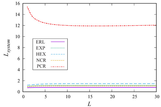
Figure 2. Impact of L on the average number of customers in the system $L_{system}$ for different $MAP$s.

However, with respect to the PCR arrivals, we see an interesting but opposite trend, namely, a decreasing one. This can intuitively be explained as follows. First, note that $L_{system}$ has a maximal value of 15.3983 when $L=1,$ which can be explained by using the fact that, when $L=1$, the secondary servers leave after serving one customer; with a probability of only 0.5 for recruitment, the queue tends to build up fast. As L is increased, secondary servers are more involved in clearing the queue, especially when the arrivals occur in spurts, and so $L_{system}$ decreases. It reaches a minimal value of 11.9757 when $L=16$ and then starts to increase due to not getting a chance to be served by the main server. For $L=30,$$L_{system}=12.0605$.

Figure 3 shows the behavior of the average number of customers with the secondary server $L_{sec}.$ As is to be expected, we see that $L_{sec}$ increases when L increases. As in the previous figure, the value of $L_{sec}$ is, generally speaking, large in the case of PCR. Only for small values of L is this value smaller for the $\mathbf{ERL}$-$\mathbf{NCR}.$ This can be explained by the high irregularity of the arrivals seen in the PCR process, which causes the system to starve, during which only the main server is busy offering services for the most part. Among $\mathbf{ERL}$-$\mathbf{HEX},$ the known effect that higher variance implies a large number of customers in the system is confirmed.

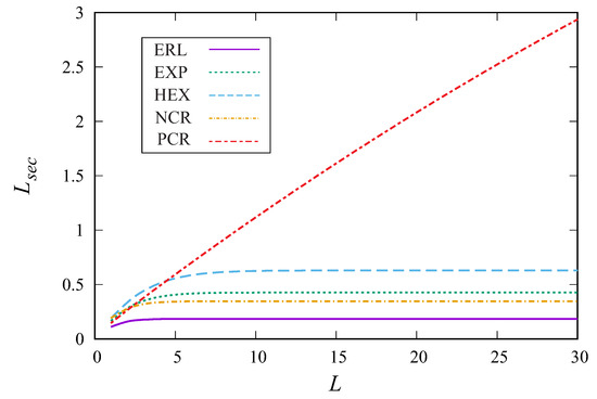
Figure 3. Dependence of the average number of customers with the secondary server $L_{sec}$ on the parameter L for different $MAP$s.

Figure 4 illustrates the behavior of the probability, $P_{idle-system}$, that the system is idle at an arbitrary moment. This figure matches Figure 2 in two respects. The first one is that it also shows a large difference in the measure when being compared to various $MAPs$. When one is interested in finding an optimal L, it is clear that it matters which measure is chosen as the objective function as well as the type of $MAPs$ used when all other parameters are fixed. For example, if we look the case of the PCR arrival process, the optimal value of L is 16 if we are tying to minimize $L_{system}.$ However, if measure $P_{idle-system}$ is the focus of the optimization problem, then $L=6$ yields the largest value for this measure.

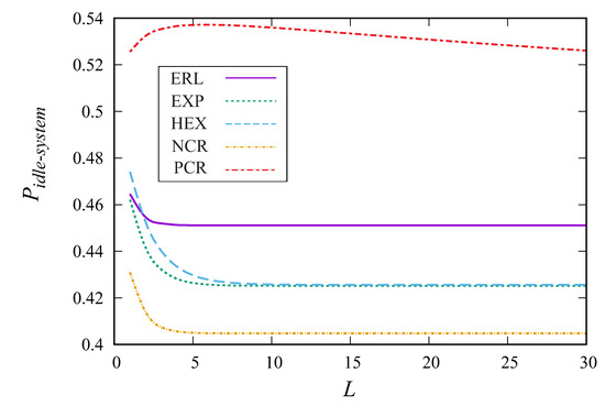
Figure 4. Dependence of the probability $P_{idle-system}$ that the system is idle at an arbitrary moment on the parameter L for different $MAP$s.

Figure 5 and Figure 6 illustrate the behavior of the probabilities $P_{idle-busy}$ and $P_{busy-idle}$, which respectively correspond to when the main server is idle with the secondary server being busy, and when the main server is busy with the secondary server being idle, at an arbitrary moment. While the first probability is increasing when L increases, the second probability is decreasing. From these figures, one can see the essential differences in these probabilities under various scenarios.

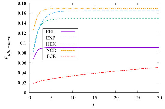
Figure 5. Dependence of the probability $P_{idle-busy}$ that the main server is idle while the secondary server is busy on the parameter L for different $MAP$s.

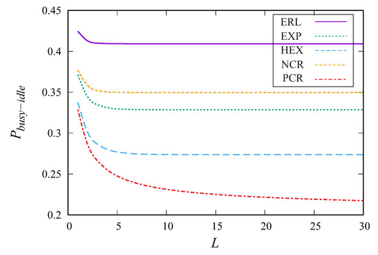
Figure 6. Dependence of the probability $P_{busy-idle}$ that the main server is busy while the secondary server is idle on the parameter L for different $MAP$s.

Illustrative Example 2:

The purpose of this example is to investigate the impact of the parameters q (recall this is the probability that a served customer refuses to act as a secondary server) and $\nu$ (this is the probability that a customer served by a secondary server is dissatisfied and sent back to the system). We fix the value of L as 10 (midpoint between the two optimal values mentioned in the first example). We also fix the service rates as ${\mathit{\mu }}_1=1$ and ${\mathit{\mu }}_2=0.5$ and investigate the dependence of several performance measures on the probabilities q and $\nu .$ We vary the values of these probabilities from 0 to 1 with step 0.05. Note that the value $q=1$ corresponds to the classic $MAP/M/1$ system with the service rate ${\mathit{\mu }}_1.$

In this example, we focus on the arrival process labeled PCR, the choice of which is based on the behavior for this process on the measures as highlighted in the first illustrative example. From Figure 7, which displays the dependence of the average number of customers in the system $L_{system}$ on the parameters q and $\nu$, we infer a number of interesting observations.

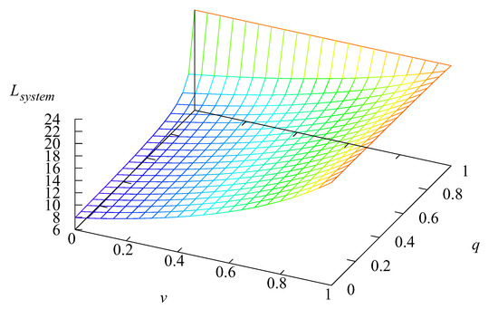
Figure 7. Dependence of the average number of customers in the system $L_{system}$ on the parameters q and $\nu$.

The value of $L_{system}$ is minimal with a value of 7.9328 when the served customer is always available to be recruited (when the system needs) and when the customer receiving service from a secondary server is always satisfied. That is the minimum attained when $q=0$ and $\nu =0$. This measure increases when either q or $\nu$ increases, and the rate of increase becomes higher when one or both q and $\nu$ approach the value 1. When $q=1$, the system transforms to the corresponding classic $MAP/M/1$ and to a system without the use of the secondary server, and $L_{system}=22.30425$ for all values of $\nu$ (as is clear). When $q=0,$ which corresponds to the case that a served customer is always recruited (when needed), even when the probability of dissatisfaction is high ($\nu =0.5$), the value of $L_{system}$ is equal to 12.91247. Therefore, the use of a secondary server essentially decreases the mean number of customers in the system by more than 40%. Also, we looked at the cut-off point, say ${\nu }^{*}$, for a dissatisfaction rate such that the classic queueing model will be better than the model proposed here. For the parameters of this example, the cut-off point is ${\nu }^{*}\simeq 0.985$, in that the dissatisfaction rate has to be more than 98.5% for the classic model to perform better.

To test further the amount of reduction in the mean number, we increased $\lambda$ by 50% to $\lambda =0.75$. Keeping all other parameters (except for the normalization of the parameters of the arrival process to arrive at this specific $\lambda$) the same, we obtained a reduction percentage of more than 52.8%. Thus, an increased load to the system will highly benefit from having a secondary server to help the system even with a high customer dissatisfaction rate of 50% with this secondary server.

Figure 8 shows the dependence of the average number of customers with the secondary server $L_{sec}$ on the parameters q and $\nu .$ This probability significantly decreases when q approaches 1 and when the customers are rarely recruited to serve as secondary servers. $L_{sec}$ has the maximal value when q is equal to zero, i.e., all customers are recruited (when needed) to become secondary servers, and when $\nu$ is close to 1. Obviously, in the latter case, almost all customers served by a secondary server have to be sent back to the system due dissatisfaction. This explains the creation of additional work to the system and should be discouraged by resorting to the classic queue as opposed to recruiting (bad) secondary servers. It is worth pointing out that such a (bad) system may reflect badly on the system itself for providing services that cannot be replicated by other (served) customers.

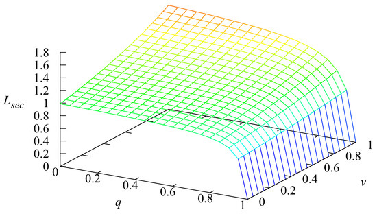
Figure 8. Dependence of the average number of customers with the secondary server $L_{sec}$ on the parameters q and $\nu$.

In Figure 9, the behavior of the probability $P_{idle-system}$ that the system is idle at an arbitrary moment as a function of q and $\nu$ is displayed. This probability has the minimal value of 0.4445 when $\nu =1$ and $q=0,$ which is intuitively clear, as having to serve customers again after going through a secondary server puts a load on the system.

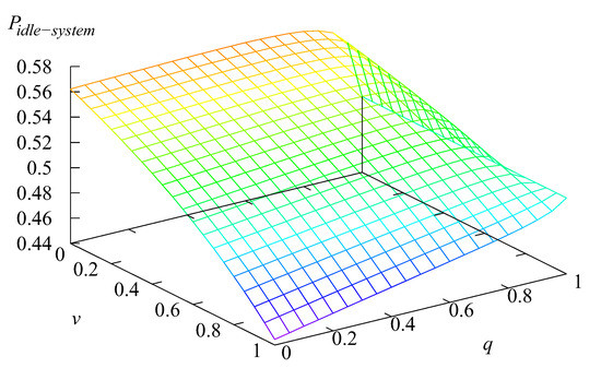
Figure 9. Dependence of the probability $P_{idle-system}$ that the system is idle at an arbitrary moment on the parameters q and $\nu$.

The probability that $P_{idle-system}$ increases when q increases and/or $\nu$ decreases: the maximal value 0.5652 of this probability is achieved when $q=0.65$ and $\nu =0.$ In the corresponding classic $MAP/M/1$ system, this measure is $P_{idle-system}=0.5$.

Figure 10 shows the behavior of the probability $P_{idle-arrival}$, as a function of q and $\nu$, that the system is idle at an arrival epoch. As can be expected, the behavior of the probability that the system is idle at an arrival epoch is similar to the behavior of the probability that the system is idle at an arbitrary moment. However, the former probability is less than the latter one. This is easily explained by the above-stated observation that in the case of PCR, wherein there are periods alternating between rare and frequent arrivals to the system, there is high likelihood that an arriving customer may be in the period of frequent arrivals leading to a high probability of seeing the system idle. It is worth pointing it out that for the corresponding classic $MAP/M/1$ system, this measure has a value of 0.358.

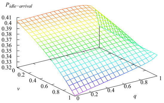
Figure 10. Dependence of the probability $P_{idle-arrival}$ that the system is idle at an arbitrary arrival moment on the parameters q and $\nu$.

Figure 11 and Figure 12 show dependencies, respectively, of the probability $P_{idle-busy}$ that the main server is idle while the secondary server is busy, and the probability $P_{busy-idle}$ that the main server is busy while the secondary server is idle on q and $\nu .$ The probability $P_{idle-busy}$ is significantly small and obviously tends to zero when probability q tends to 1. On the other hand, the probability $P_{busy-idle}$ appears to be much larger than $P_{idle-busy}.$ The probability $P_{busy-idle}$ tends to increase when q is increased to 1.

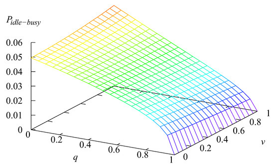
Figure 11. Dependence of the probability $P_{idle-busy}$ that the main server is idle while the secondary server is busy on the parameters q and $\nu$.

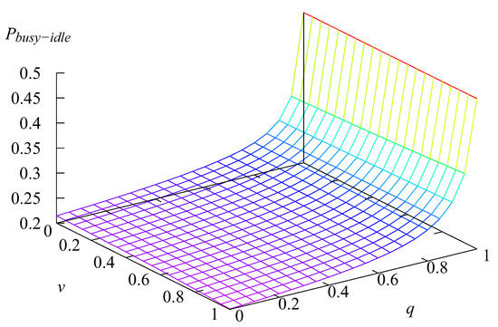
Figure 12. Dependence of the probability $P_{busy-idle}$ that the main server is busy while the secondary server is idle on the parameters q and $\nu$.

Illustrative Example 3:

In this final example, we investigate the impact of the varying the service rates ${\mathit{\mu }}_1$ and ${\mathit{\mu }}_2$ when all other parameters are fixed. Towards this end, we fix $L=10$, $q=0.5,$$\nu =0.4$, and $\lambda =0.5$. The rates ${\mathit{\mu }}_1$ and ${\mathit{\mu }}_2$ are varied from 0.25 to 2.0 in increments of 0.05. It is worth mentioning that, to fulfill the ergodicity condition (see Equation (5)), we additionally restrict the value of ${\mathit{\mu }}_2$ whenever ${\mathit{\mu }}_1$ is small. In particular, when ${\mathit{\mu }}_1=0.25,$ the minimal value of the rate ${\mathit{\mu }}_2$ is chosen (with the pre-described above step as 0.05) to be no less than 0.65. When ${\mathit{\mu }}_1=0.3,$ the rate ${\mathit{\mu }}_2$ is chosen to be no less than 0.45. When ${\mathit{\mu }}_1=0.35,$ the rate ${\mathit{\mu }}_2$ is chosen to be no less than 0.3. Only for ${\mathit{\mu }}_1\ge 0.4$ can the value of ${\mathit{\mu }}_2$ be varied from 0.25 as originally pointed out.

With the above restrictions on the choice of ${\mathit{\mu }}_1$ and ${\mathit{\mu }}_2$, we display in Figure 13 and Figure 14 the dependence of the measure $L_{system}$ on ${\mathit{\mu }}_1$ and ${\mathit{\mu }}_2.$ In Figure 13, most of the surface showing the dependence looks flat. This is due to the fact that, for many combinations of the parameter values with small rate ${\mathit{\mu }}_1$, the ergodicity condition is violated and the measure $L_{system}$ becomes very large. Therefore, in Figure 14, the dependence of $L_{system}$ on ${\mathit{\mu }}_1$ and ${\mathit{\mu }}_2$ is displayed only for non-small values of ${\mathit{\mu }}_1.$ Clearly, one can see a decreasing trend as $L_{system}$ quickly decreases when ${\mathit{\mu }}_1$ increases for fixed ${\mathit{\mu }}_2$ and vice-versa.

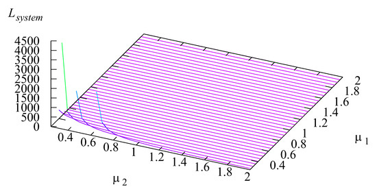
Figure 13. Dependence of the average number of customers in the system $L_{system}$ on the parameters ${\mathit{\mu }}_1$ and ${\mathit{\mu }}_2$.

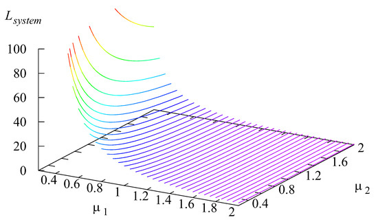
Figure 14. Dependence of the average number of customers in the system $L_{system}$ on the parameters ${\mathit{\mu }}_1$ and ${\mathit{\mu }}_2$.

Figure 15 shows the behavior of the average number of customers with the secondary server $L_{sec}.$ The value of $L_{sec}$ is maximized with a value of about 5 when ${\mathit{\mu }}_1$ and ${\mathit{\mu }}_2$ are small. This is intuitively clear since for small values of ${\mathit{\mu }}_1$ and ${\mathit{\mu }}_2$, the ergodicity condition is close to being violated, causing a high recruitment rate for secondary servers who in all likelihood before leaving the system will serve a group of size $L=10$. Thus, the average number of customers in service at an arbitrary moment is about 5. With an increase in ${\mathit{\mu }}_1$ and ${\mathit{\mu }}_2,$ the value of $L_{sec}$ decreases as one would expect. For small values of ${\mathit{\mu }}_1$, the decrease is significant as ${\mathit{\mu }}_2$ is increased; for larger values of ${\mathit{\mu }}_1,$ we notice an insignificant rate of decrease in $L_{sec}$ with an increase in ${\mathit{\mu }}_2$.

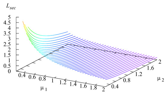
Figure 15. Dependence of the average number of customers with the secondary server $L_{sec}$ on the parameters ${\mathit{\mu }}_1$ and ${\mathit{\mu }}_2$.

Figure 16 and Figure 17 illustrate the behavior of $P_{idle-system}$ and $P_{idle-arrival}.$ As in the previous example, $P_{idle-arrival}$ is less than that of $P_{idle-system}.$

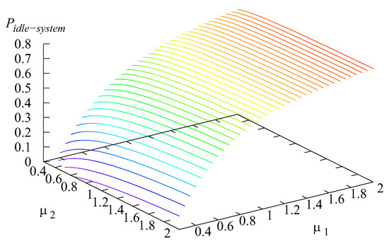
Figure 16. Dependence of the probability $P_{idle-system}$ that the system is idle at an arbitrary moment on the parameters ${\mathit{\mu }}_1$ and ${\mathit{\mu }}_2$.

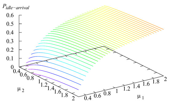
Figure 17. Dependence of the probability $P_{idle-arrival}$ that the system is idle at an arbitrary arrival moment on the parameters q and $\nu$.

Figure 18 and Figure 19 illustrate the behavior of $P_{idle-busy}$ and $P_{busy-idle}.$ These performance characteristics can be quite interesting if the economic arguments are taken into account. For example, if the work of the secondary server is not gratis, then the analysis of the secondary server to stay idle or busy while the main server is busy or idle should shed more light and will be a topic of interest for a future study.

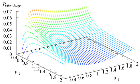
Figure 18. Dependence of the probability $P_{idle-busy}$ that the main server is idle while the secondary server is busy on the parameters q and $\nu$.

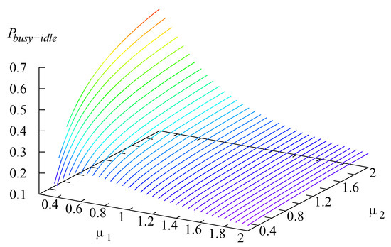
Figure 19. Dependence of the probability $P_{busy-idle}$ that the main server is busy while the secondary server is idle on the parameters ${\mathit{\mu }}_1$ and ${\mathit{\mu }}_2$.

6. Conclusions

In this paper, we analyzed a queueing system in which there is an opportunity to recruit a (served) customer as a secondary server to help the main server by assigning a group of a finite number of waiting customers. The arrival process is modeled using a versatile Markovian point process, $MAP.$ The possibility of customer dissatisfaction with the service provided by the secondary server causing those customers to be fed back into the system is taken into account. The steady state analysis of the multi-dimensional Markov chain describing behavior of the system is implemented, and illustrative numerical results potentially useful for making managerial decisions are presented.

The model studied in this paper can be generalized in a number of ways. For example, (i) the service provided by the secondary server can be done in groups; (ii) relax the assumption of having only one secondary server to more than one and see the impact of just increasing it to, say, 2; (iii) use phase-type services possibly with different representations for the main and secondary server; (iv) incorporate impatience of the customers in both the main and secondary buffers; (v) implement a recruitment process depending on the observed queue length based on a threshold-type control policy; (vi) allow group arrivals; and finally (vii) incorporate the possibility of recruiting many secondary servers with two types of customers such that only one type will qualify to act as secondary servers.

References

- Chaurasia, N.; Kumar, M.; Chaudhry, R.; Verma, O.P. Comprehensive survey on energy-aware server consolidation techniques in cloud computing. J. Supercomput. 2021, 77, 11682–11737. [Google Scholar] [CrossRef]
- Maccio, V.J.; Down, D.G. Structural properties and exact analysis of energy-aware multiserver queueing systems with setup times. Perform. Eval. 2018, 121, 48–66. [Google Scholar] [CrossRef]
- Mitrani, I. Trading power consumption against performance by reserving blocks of servers. In Computer Performance Engineering; Springer: Berlin/Heidelberg, Germany, 2013; pp. 1–15. [Google Scholar]
- Mitrani, I. Managing performance and power consumption in a server farm. Ann. Oper. Reasearch 2013, 202, 121–134. [Google Scholar] [CrossRef]
- Mitrani, I. Service center trade-offs between customers impatience and power consumation. Perform. Eval. 2011, 68, 1222–1231. [Google Scholar] [CrossRef]
- Lui, J.C.S.; Golubchik, L. Stochastic complement analysis of multi-server threshold queues with hysteresis. Perform. Eval. 1999, 35, 19–48. [Google Scholar] [CrossRef]
- Gortsev, A.M.; Nazarov, A.A.; Terpugov, A.F. Control and Adaptation in Queueing Systems; Tomsk University Press: Tomsk, Russia, 1978. (In Russian) [Google Scholar]
- Rykov, V.; Efrosinin, D. Optimal Control of Queueing Systems with Heterogeneous Servers. Queueing Syst. 2004, 46, 389–407. [Google Scholar] [CrossRef]
- Ibe, O.C.; Keilson, J. Multi-server threshold queues with hysteresis. Perform. Eval. 1995, 21, 185–213. [Google Scholar] [CrossRef]
- Li, H.; Yang, T. Queues with a variable number of servers. Eur. J. Oper. Res. 2000, 124, 615–628. [Google Scholar] [CrossRef]
- Chou, C.F.; Golubchik, L.; Lui, J.C.S. Multiclass Multiserver Threshold-Based Systems: A Study of Noninstantaneous Server Activation. IEEE Trans. Parallel Distrib. Syst. 2007, 18, 96–110. [Google Scholar] [CrossRef]
- Kitaev, M.Y.; Rykov, V.V. Controlled Queueing Systems; CRC Press: New York, NY, USA, 1995. [Google Scholar]
- Rykov, V.V. Monotone Control of Queueing Systems with Heterogeneous Servers. Queueing Syst. 2001, 37, 391–403. [Google Scholar]
- Efrosinin, D.; Breuer, L. Threshold policies for controlled retrial queues with heterogeneous servers. Ann. Oper. Res. 2006, 141, 139–162. [Google Scholar] [CrossRef]
- Nobel, R.D.; Tijms, H.C. Optimal control of a queueing system with heterogeneous servers and setup costs. IEEE Trans. Autom. Control 2000, 45, 780–784. [Google Scholar] [CrossRef]
- Nobel, R. A retrial queueing system with a variable number of active servers: Dynamic manpower planning in a call center. In International Conference on Queueing Theory and Network Applications; Springer: Cham, Switzerland, 2018; pp. 33–47. [Google Scholar]
- Lin, W.; Kumar, P. Optimal control of a queueing system with two heterogeneous servers. IEEE Trans. Autom. Control 1984, 29, 696–703. [Google Scholar] [CrossRef]
- Walrand, J. A note on “Optimal control of a queuing system with two heterogeneous servers”. Syst. Control Lett. 1984, 4, 131–134. [Google Scholar] [CrossRef]
- Schwartz, C.; Pries, R.; Tran-Gia, P. A queuing analysis of an energy-saving mechanism in data centers. In Proceedings of the International Conference on Information Network, Bali, Indonesia, 1–3 February 2012; pp. 70–75. [Google Scholar]
- Ivaneshkin, A.I. Optimizing a multiserver queuing system with a variable number of servers. Cybern. Syst. Anal. 2007, 43, 542–548. [Google Scholar] [CrossRef]
- Efrosinin, D.; Sztrik, J. An algorithmic approach to analysing the reliability of a controllable unreliable queue with two heterogeneous servers. Eur. J. Oper. Res. 2018, 271, 934–952. [Google Scholar] [CrossRef]
- Efrosinin, D.; Stepanova, N. Estimation of the optimal threshold policy in a queue with heterogeneous servers using a heuristic solution and artificial neural networks. Mathematics 2021, 9, 1267. [Google Scholar] [CrossRef]
- Klimenok, V.; Dudin, A.; Samouylov, K. Analysis of the BMAP/PH/N queueing system with backup servers. Appl. Math. Model. 2018, 57, 64–84. [Google Scholar] [CrossRef]
- Dudin, A.; Dudina, O.; Dudin, S.; Gaidamaka, Y. Self-service system with rating dependent arrivals. Mathematics 2022, 10, 297. [Google Scholar] [CrossRef]
- Artalejo, J.R.; Gomez-Correl, A.; He, Q.M. Markovian arrivals in stochastic modelling: A survey and some new results. SORT-Stat. Oper. Res. Trans. 2010, 34, 101–144. [Google Scholar]
- Bladt, M.; Nielsen, B.F. Matrix-Exponential Distributions in Applied Probability; Springer: Boston, MA, USA, 2017. [Google Scholar]
- Chakravarthy, S.R. The Batch Markovian Arrival Process: A Review and Future Work. Adv. Probab. Theory Stoch. Process. 2001, 1, 21–49. [Google Scholar]
- Chakravarthy, S.R. Markovian Arrival Processes. In Wiley Encyclopedia of Operations Research and Management Science; Wiley: Hoboken, NJ, USA, 2010. [Google Scholar]
- Chakravarthy, S.R. Introduction to Matrix-Analytic Methods in Queues 1: Analytical and Simulation Approach—Basics; ISTE Ltd.: London, UK; John Wiley and Sons: New York, NY, USA, 2022. [Google Scholar]
- Chakravarthy, S.R. Introduction to Matrix-Analytic Methods in Queues 2: Analytical and Simulation Approach—Queues and Simulation; ISTE Ltd.: London, UK; John Wiley and Sons: New York, NY, USA, 2022. [Google Scholar]
- Dudin, A.N.; Klimenok, V.I.; Vishnevsky, V.M. The Theory of Queuing Systems with Correlated Flows; Springer Nature: Berlin/Heidelberg, Germany, 2020. [Google Scholar]
- He, Q.-M. Fundamentals of Matrix-Analytic Methods; Springer: New York, NY, USA, 2014. [Google Scholar]
- Latouche, G.; Ramaswami, V. Introduction to Matrix Analytic Methods in Stochastic Modeling; SIAM: Philadelphia, PA, USA, 1999. [Google Scholar]
- Lucantoni, D.; Meier-Hellstern, K.S.; Neuts, M.F. A single-server queue with server vacations and a class of nonrenewal arrival processes. Adv. Appl. Probab. 1990, 22, 676–705. [Google Scholar] [CrossRef]
- Lucantoni, D. New results on the single server queue with a batch Markovian arrival process. Stoch. Model. 1991, 7, 1–46. [Google Scholar] [CrossRef]
- Neuts, M.F. A versatile Markovian point process. J. Appl. Probab. 1979, 16, 764–779. [Google Scholar] [CrossRef]
- Neuts, M.F. Matrix-Geometric Solutions in Stochastic Models; The Johns Hopkins University Press: Baltimore, MD, USA, 1981. [Google Scholar]
- Neuts, M.F. Structured Stochastic Matrices of M/G/1 Type and Their Applications; Marcel Dekker: New York, NY, USA, 1989. [Google Scholar]
- Neuts, M.F. Models based on the Markovian arrival processes. IEICE Trans. Commun. 1992, E75-B, 1255–1265. [Google Scholar]
- Naumov, V.; Gaidamaka, Y.; Yarkina, N.; Samouylov, K. Matrix and Analytical Methods for Performance Analysis of Telecommunication Systems; Springer Nature: Berlin/Heidelberg, Germany, 2021. [Google Scholar]
- Chakravarthy, S.R. A Multi-server Queueing Model with Markovian Arrivals and Multiple Thresholds. Asia-Pac. J. Oper. Res. 2007, 24, 223–243. [Google Scholar] [CrossRef]
- Chakravarthy, S.R.; Agnihothri, S.R. A Server Backup Model with Markovian Arrivals and Phase Type Services (with). Eur. J. Oper. Res. 2008, 184, 584–609. [Google Scholar] [CrossRef]
- Chakravarthy, S.R. A stochastic model for a dynamic service facility with threshold and lead time. In Proceedings of the Second International Conference on Stochastic Modelling and Simulation, Tamil Nadu, India, 17–19 December 2012; pp. 3–22. [Google Scholar]
- Chakravarthy, S.R.; Kulshrestha, R. A queueing model with server breakdowns, repairs, vacations, and backup server. Oper. Res. Perspect. 2020, 7, 100131. [Google Scholar] [CrossRef]
- Kim, C.S.; Dudin, A.; Dudin, S.; Dudina, O. Hysteresis control by the number of active servers in queueing system with priority service. Perform. Eval. 2016, 101, 20–33. [Google Scholar] [CrossRef]
- Chakravarthy, S.R.; Dudin, A.N. A Queueing Model for Crowdsourcing. J. Oper. Res. Soc. 2017, 68, 221–236. [Google Scholar] [CrossRef]
- Arslan, A.M.; Agatz, N.; Kroon, L.; Zuidwijk, R. Crowdsourced delivery—A dynamic pickup and delivery problem with ad hoc drivers. Transp. Sci. 2019, 53, 222–235. [Google Scholar] [CrossRef]
- Savelsbergh, M.W.; Ulmer, M.W. Challenges and opportunities in crowdsourced delivery planning and operations. 4OR 2022, 20, 1–21. [Google Scholar] [CrossRef]
- Sun, L.; Yang, Q.; Chen, X.; Chen, Z. RC-chain: Reputation-based crowdsourcing blockchain for vehicular networks. J. Netw. Comput. Appl. 2021, 176, 102956. [Google Scholar] [CrossRef]
- Fatehi, S.; Wagner, M.R. Crowdsourcing last-mile deliveries. Manuf. Serv. Oper. Manag. 2022, 24, 791–809. [Google Scholar] [CrossRef]
- Graham, A. Kronecker Products and Matrix Calculus with Applications; Ellis Horwood: Cichester, UK, 1981. [Google Scholar]
- Steeb, W.-H.; Hardy, Y. Matrix Calculus and Kronecker Product; World Scientific Publishing: Singapore, 2011. [Google Scholar]
- Horn, R.A.; Johnson, C.R. Topics in Matrix Analysis; Cambridge University Press: Cambridge, UK, 1991. [Google Scholar]
- Zhang, H.; Ding, F. On the Kronecker products and their applications. J. Appl. Math. 2013, 2013, 296185. [Google Scholar] [CrossRef]
- Gantmacher, F.R. Theory of Matrices, 1st ed.; Science USSR: Moscow, Russia, 1967. [Google Scholar]
Disclaimer/Publisher’s Note: The statements, opinions and data contained in all publications are solely those of the individual author(s) and contributor(s) and not of MDPI and/or the editor(s). MDPI and/or the editor(s) disclaim responsibility for any injury to people or property resulting from any ideas, methods, instructions or products referred to in the content. |
© 2023 by the authors. Licensee MDPI, Basel, Switzerland. This article is an open access article distributed under the terms and conditions of the Creative Commons Attribution (CC BY) license (https://creativecommons.org/licenses/by/4.0/).