Article

A New Alpha Power Cosine-Weibull Model with Applications to Hydrological and Engineering Data

by
Abdulaziz S. Alghamdi
1 and
M. M. Abd El-Raouf
2,*
1
Department of Mathematics, College of Science & Arts, King Abdulaziz University, P.O. Box 344, Rabigh 21911, Saudi Arabia
2
Basic and Applied Science Institute, Arab Academy for Science, Technology and Maritime Transport (AASTMT), Alexandria P.O. Box 1029, Egypt
*
Author to whom correspondence should be addressed.
Mathematics 2023, 11(3), 673; https://doi.org/10.3390/math11030673
Submission received: 12 December 2022 / Revised: 19 January 2023 / Accepted: 24 January 2023 / Published: 28 January 2023
(This article belongs to the Special Issue Advances in Applied Probability and Statistical Inference)

Abstract

:
Modifying the existing probability models in the literature and introducing new extensions of the existing probability models is a prominent and interesting research topic. However, in the most recent era, the extensions of the probability models via trigonometry methods have received great attention. This paper also offers a novel trigonometric version of the Weibull model called a new alpha power cosine-Weibull (for short, “NACos-Weibull”) distribution. The NACos-Weibull distribution is introduced by incorporating the cosine function. Certain distributional properties of the NACos-Weibull model are derived. The estimators of the NACos-Weibull model are derived by implementing the maximum likelihood approach. Three simulation studies are provided for different values of the parameters of the NACos-Weibull distribution. Finally, to demonstrate the effectiveness of the NACos-Weibull model, three applications from the hydrological and engineering sectors are considered.

1. Introduction

In the class of probability distributions (for short, “PDs”) defined on R + , the Weibull (for short, “Wei”) has a special place. The consideration of the Wei distribution is one of the first selections of researchers to implement for analyzing data in the (i) business and financial sectors Silahli et al. [1] ), (Teamah et al. [2]), (Ahmad et al. [3])], (ii) hydrological fields (Chaito and Khamkong [4]), (iii) irrigation Shahmari (et al. [5]). (iv) meteorology (Suwarno and Zambak [6]), and (v) Engineering (Al-Babtain et al. [7]).
Suppose X has the Wei distribution represented by X W ϕ , δ , with cumulative distribution function (CDF) expressed by B x ; ψ and probability density function (PDF) b x ; ψ . Then, the CDF of X is
B x ; ψ = 1 e ϕ x δ x 0 0 o t h e r w i s e ,
where ψ = ϕ , δ , ϕ > 0 , and δ > 0 . Corresponding to B x ; ψ in Equation (1), the PDF is
b x ; ψ = δ ϕ x δ 1 e ϕ x δ x > 0 0 o t h e r w i s e .
Due to certain limitations of the Wei distribution (i.e., limited data modeling and monotonic hazard function, etc.), researchers have been trying to develop its updated versions. Therefore, to bring more flexibility to W ϕ , δ , its numerous extensions have been studied. For example, Strzelecki [8] introduced a 3-parameter updated version of the Wei distribution for determining the fatigue life for different stress levels. Sindhu and Atangana [9] implemented the exponentiated inverse Weibull (EI-Wei) distribution for reliability analysis. Abubakar et al. [10] consider a modified form of the Wei model for analyzing investment returns. Kovacs et al. [11] also considered a modified Weibull model for predicting the service life and spare parts forecast on an industrial scale. Liu et al. [12] used a new version of the Wei distribution to analyze the COVID-19 phenomena. Dessalegn et al. [13] implemented another modified form of the Wei distribution for investigating the bamboo fibrous tensile strength. Alyami et al. [14] studied a Topp–Leone modified Weibull distribution for analyzing the medical and engineering data sets. Bakr et al. [15] developed a novel method for generalizing the existing probability distributions for modeling data in real-life/applied sectors.
In this paper, we also contribute to improving the distributional flexibility of the Wei distribution for analyzing the hydrological and engineering data sets. The model studied in this work is called a new alpha power cosine-Weibull (for short, “NACos-Weibull”) distribution. The NACos-Weibull distribution is introduced by implementing a method based on the trigonometry function, namely alpha power transformed cosine-X (for short, “APTCos-X”) family.
Let X has the APTCos-X family with CDF G x ; α , ψ . Then G x ; α , ψ of the APTCos-X family has the below expression
G x ; α , ψ = α cos π 2 π B x ; ψ 2 1 α 1 , x R , α > 0 , α 1 ,
with PDF g x ; α , ψ given by
g x ; α , ψ = π log α b x ; ψ sin π 2 π B x ; ψ 2 2 α 1 α cos π 2 π B x ; ψ 2 , x R , α > 0 , α 1 ,
where the quantity ψ is a parameter vector associated with baseline CDF B x ; ψ , and d d x B x ; ψ = b x ; ψ .
Corresponding to G x ; α , ψ and g x ; α , ψ , the survival function (SF) S x ; α , ψ = 1 G x ; α , ψ , hazard function (HF) h x ; α , ψ = g x ; α , ψ S x ; α , ψ , cumulative HF (CHF) H x ; α , ψ = log 1 G x ; α , ψ , and reverse HF (RHF) r x ; α , ψ = g x ; α , ψ G x ; α , ψ of the APTCos-X approach are, respectively, given by
S x ; α , ψ = α α cos π 2 π B x ; ψ 2 α 1 ,
h x ; α , ψ = π log α b x ; ψ sin π 2 π B x ; ψ 2 2 α α cos π 2 π B x ; ψ 2 α cos π 2 π B x ; ψ 2 ,
H x ; α , ψ = log α α cos π 2 π B x ; ψ 2 α 1 ,
and
r x ; α , ψ = π log α b x ; ψ sin π 2 π B x ; ψ 2 2 α cos π 2 π B x ; ψ 2 1 α cos π 2 π B x ; ψ 2 .
In the next section, we are motivated to introduce the proposed NACos-Weibull distribution by using Equation (1) in Equation (3). Certain basic functions of the NACos-Weibull are presented. In addition to the basic functions, the plots for the density function of the NACos-Weibull are also obtained. In Section 3, we derive some distributional properties of the NACos-Weibull distribution. Section 4 is devoted to derive the maximum likelihood estimators and simulation study of the NACos-Weibull distribution. Section 5 deals with the practical illustration of the NACos-Weibull distribution by considering the hydrological and engineering data sets. Section 6 provides some final concluding remarks.

2. A NACos-Weibull Distribution

This section offers an introduction to the NACos-Weibull distribution by providing its basic expressions. Let X has the NACos-Weibull distribution with CDF G x ; α , ψ , if it is
G x ; α , ψ = α cos π 2 π 1 e ϕ x δ 2 1 α 1 x 0 0 o t h e r w i s e ,
with PDF g x ; α , ψ expressed by
g x ; α , ψ = π log α δ ϕ x δ 1 e ϕ x δ sin π 2 π 1 e ϕ x δ 2 2 α 1 α cos π 2 π 1 e ϕ x δ 2 x > 0 0 o t h e r w i s e .
The NACos-Weibull distribution is a useful modification of the Weibull model with a single extra additional parameter.
Figure 1 offers the visual behavior of the NACos-Weibull distribution by plotting the shape of its PDF g x ; α , ψ . From Figure 1, it can be seen that g x ; α , ψ of the NACos-Weibull model has different shapes. These shapes include (i) decreasing form (golden curve shape), (ii) symmetrical form (blue curve shape), (iii) right-skewed form (red curve shape), and (iv) left-skewed forms (green and black line shapes).
Corresponding to G x ; α , ψ (see Equation (5)) and g x ; α , ψ (see Equation (6)), the expressions for the SF, CHF, HF, and RHF of the NACos-Weibull are provided by
S x ; α , ψ = α α cos π 2 π 1 e ϕ x δ 2 α 1 ,
H x ; α , ψ = log α α cos π 2 π 1 e ϕ x δ 2 α 1 ,
h x ; α , ψ = π log α δ ϕ x δ 1 e ϕ x δ sin π 2 π 1 e ϕ x δ 2 2 α α cos π 2 π 1 e ϕ x δ 2 α cos π 2 π 1 e ϕ x δ 2 ,
and
r x ; α , ψ = π log α δ ϕ x δ 1 e ϕ x δ sin π 2 π 1 e ϕ x δ 2 2 α cos π 2 π 1 e ϕ x δ 2 1 α cos π 2 π 1 e ϕ x δ 2 ,
respectively.
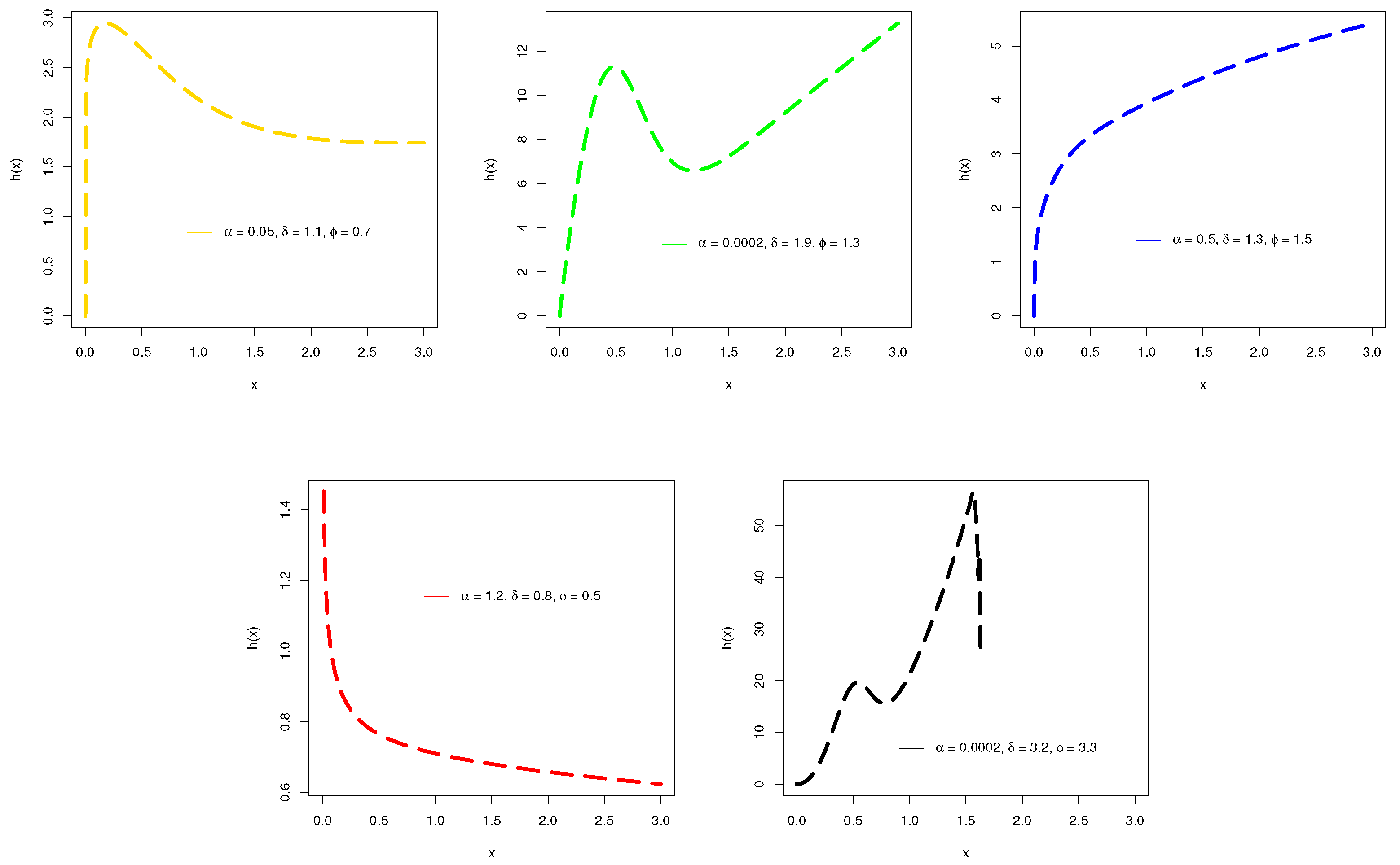
Figure 2 offers the visual behavior of the HF h x ; α , ψ of the NACos-Weibull distribution. From Figure 2, it can be seen that h x ; α , ψ of the NACos-Weibull model has different shapes. These shapes include (i) unimodal form (golden curve shape), (ii) modified unimodal form (green curve shape), (iii) increasing form (blue curve shape), (iv) decreasing form (red line shapes), and (v) bimodal form (black line shape).

3. Distributional Properties

Some basic distributional properties of the NACos-Weibull distribution are derived in this section. These properties include the (i) quantile function (QF), (ii) kth moment, (iii) characteristic function (CF), and (iv) moment generating function (MGF).

3.1. The QF

For a series of practical applications, especially for generating random numbers, it is crucial to derive the QF of a statistical distribution. Using the inverse version of Equation (5), we obtain the QF of the NACos-Weibull distribution as given by
Q u = 1 ϕ log 2 π cos 1 Δ 1 / δ ,
where
Δ = log 1 + α 1 u log α .
Using the expression of QF presented in Equation (7), we can derive several distributional properties of the NACos-Weibull model. These distributional properties may include the (i) median (it is also called the 2nd quartile) denoted by Q 2 , (ii) 1st quartile denoted by Q 1 , and (iii) 3rd quartile denoted by Q 3 . These quartiles i . e . , Q 1 , Q 2 , Q 3 can be utilized to obtain further distributional properties of the NACos-Weibull model. Galton [16] and Moors [17] used the quantile functions to obtain the measures of skewness and kurtosis, respectively. We can use the values of the quartiles to obtain the Galton skewness (GS) and Moor kurtosis (MK) of the NACos-Weibull distribution. The expressions of the GS and MK are respectively given by
G S = Q 6 / 8 2 Q 4 / 8 + Q 2 / 8 Q 6 / 8 Q 2 / 8 ,
and
M K = Q 7 / 8 Q 5 / 8 Q 1 / 8 + Q 3 / 8 Q 6 / 8 Q 2 / 8 .

3.2. The kth Moment

The moments play a significant role to derive the basic properties of probability distributions. With the help of moments, we can find the location or mean point. They can also be used to obtain the variance. Furthermore, the skewness and kurtosis of probability models can also be obtained with the help of moments. Therefore, we derive the kth moment of the NACos-Weibull distribution. Let X has the NACos-Weibull distribution, then, its kth moment is computed as
μ k = Ω x k g x ; α , ψ d x .
Using Equation (4) in Equation (8), we have
μ k = Ω x k π log α b x ; ψ sin π 2 π B x ; ψ 2 2 α 1 α cos π 2 π B x ; ψ 2 d x ,
μ k = j = 0 log α j j ! Ω x k π log α b x ; ψ sin π 2 π B x ; ψ 2 2 α 1 cos π 2 π B x ; ψ 2 j d x ,
μ k = j = 0 π log α j + 1 j ! 2 α 1 Ω x k b x ; ψ 1 cos π 2 π B x ; ψ 2 cos π 2 π B x ; ψ 2 j d x ,
μ k = j = 0 π log α j + 1 j ! 2 α 1 Ω x k b x ; ψ cos π 2 π B x ; ψ 2 j d x j = 0 π log α j + 1 j ! 2 α 1 Ω x k b x ; ψ cos π 2 π B x ; ψ 2 j + 1 d x .
Using Equations (1) and (2) in Equation (9), we have
μ k = j = 0 π log α j + 1 j ! 2 α 1 0 δ ϕ x k + δ 1 e ϕ x δ cos π 2 e ϕ x δ j d x j = 0 π log α j + 1 j ! 2 α 1 0 δ ϕ x k + δ 1 e ϕ x δ cos π 2 e ϕ x δ j + 1 d x ,
μ k = j = 0 π log α j + 1 j ! 2 α 1 κ j x j = 0 π log α j + 1 j ! 2 α 1 κ j + 1 x ,
where κ j x and κ j + 1 x are, respectively, given by
κ j x = 0 δ ϕ x k + δ 1 e ϕ x δ cos π 2 e ϕ x δ j d x ,
and
κ j + 1 x = 0 δ ϕ x k + δ 1 e ϕ x δ cos π 2 e ϕ x δ j + 1 d x .

3.3. The MGF

The approach of MGF is another useful way for generating the basic moments of any probability distribution. It may be expressed by M t x = E e t x . So, the expression of the NACos-Weibull distribution, say M t x , is derived as
M t x = E e t x = k = 0 t k k ! Ω x k g x ; α , ψ d x .
Using Equation (4) in Equation (10), we have
M t x = k = 0 t k k ! Ω x k π log α b x ; ψ sin π 2 π B x ; ψ 2 2 α 1 α cos π 2 π B x ; ψ 2 d x .
Using Equations (1) and (2) in Equation (11), and solving, we get
M t x = j , k = 0 π log α j + 1 t k k ! j ! 2 α 1 κ j x j , k = 0 π log α j + 1 t k k ! j ! 2 α 1 κ j + 1 x .

3.4. The CF

Another useful approach for generating the basic moments of any probability distribution is called the CF. Here, we represent the CF by η i t x . Let X has the NAC-Weibull distribution, then the CF of the NACos-Weibull distribution, say η i t x , is derived as
η i t x = E e ( i t ) x = k = 0 ( i t ) k k ! Ω x k g x ; α , ψ d x .
Using Equation (4) in Equation (12), we have
η i t x = k = 0 ( i t ) k k ! Ω x k π log α b x ; ψ sin π 2 π B x ; ψ 2 2 α 1 α cos π 2 π B x ; ψ 2 d x .
Using Equations (1) and (2) in Equation (13), and solving, we get
η i t x = j , k = 0 π log α j + 1 ( i t ) k k ! j ! 2 α 1 κ j x j , k = 0 π log α j + 1 ( i t ) k k ! j ! 2 α 1 κ j + 1 x .

4. Estimation and Simulation

This section carries two aims including the derivation of the maximum likelihood estimators (MLEs) δ ^ M L E , ϕ ^ M L E , α ^ M L E of the NACos-Weibull distribution and simulation study to judge the performances of δ ^ M L E , ϕ ^ M L E , and α ^ M L E .

4.1. Estimation

In this subsection, we accomplish the first aim of this section by deriving the MLEs of the NACos-Weibull distribution. Let x 1 , x 2 , , x n be a set of n observed values from g x ; α , ψ of the NACos-Weibull distribution. Then, corresponding to g x ; α , ψ in Equation (4), the likelihood function (LF) expressed by κ α , ψ | x ̲ is given by
κ α , ψ | x ̲ = i = 1 n g x i ; α , ψ .
Using Equation (6) in Equation (14), we have
κ α , ψ | x ̲ = i = 1 n π log α δ ϕ x i δ 1 e ϕ x i δ sin π 2 π 1 e ϕ x i δ 2 2 α 1 α cos π 2 π 1 e ϕ x i δ 2 .
Linked to κ α , ψ | x ̲ of the NACos-Weibull distribution, the log LF (LLF) expressed by η x ̲ | α , ψ is given by
η α , ψ | x ̲ = n log π + n log log α + n log δ + n log ϕ + δ 1 i = 1 n log x i ϕ i = 1 n x i δ n log 2 α 2 + i = 1 n log sin π 2 π 1 e ϕ x i δ 2 + i = 1 n cos π 2 π 1 e ϕ x i δ 2 log α .
Corresponding to η α , ψ | x ̲ of the NACos-Weibull distribution, the partial derivatives are respectively provided by
δ η α , ψ | x ̲ = π ϕ 2 i = 1 n log x i x i δ e ϕ x i δ sin π 2 π 1 e ϕ x i δ 2 log α π ϕ 2 i = 1 n log x i x i δ e ϕ x i δ cot π 2 π 1 e ϕ x i δ 2 + n δ + i = 1 n log x i ϕ i = 1 n log x i x i δ ,
ϕ η α , ψ | x ̲ = n ϕ i = 1 n x i δ π 2 i = 1 n x i δ e ϕ x i δ cot π 2 π 1 e ϕ x i δ 2 + π 2 i = 1 n x i δ e ϕ x i δ sin π 2 π 1 e ϕ x i δ 2 log α ,
and
α η α , ψ | x ̲ = n log α α 2 n 2 α 2 + i = 1 n 1 α cos π 2 π 1 e ϕ x i δ 2 .
Solving the expressions δ η α , ψ | x ̲ = 0 , ϕ η α , ψ | x ̲ = 0 , and α η α , ψ | x ̲ = 0 simultaneously yield the estimators δ ^ M L E , ϕ ^ M L E , α ^ M L E of the parameters δ , ϕ , α .
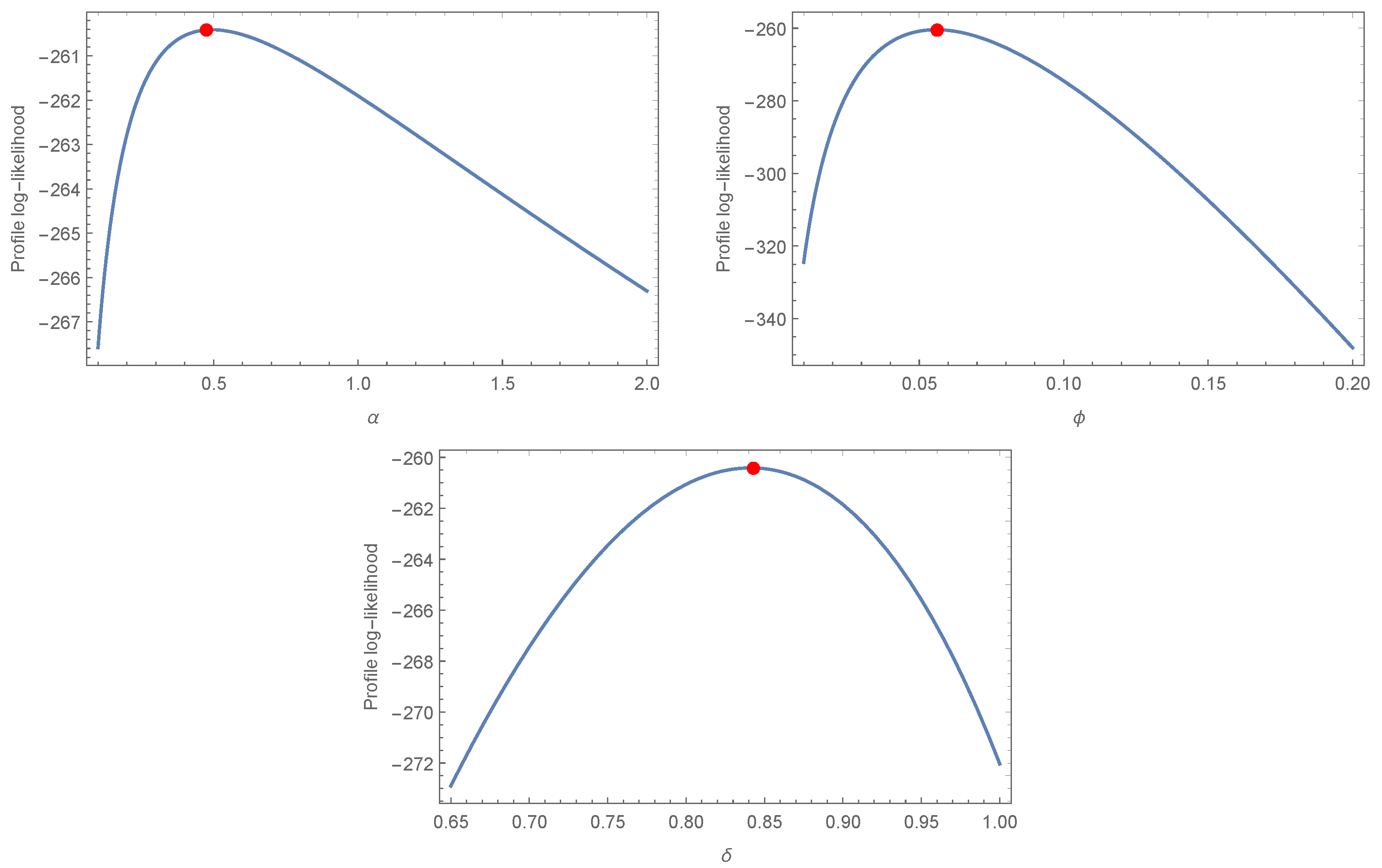
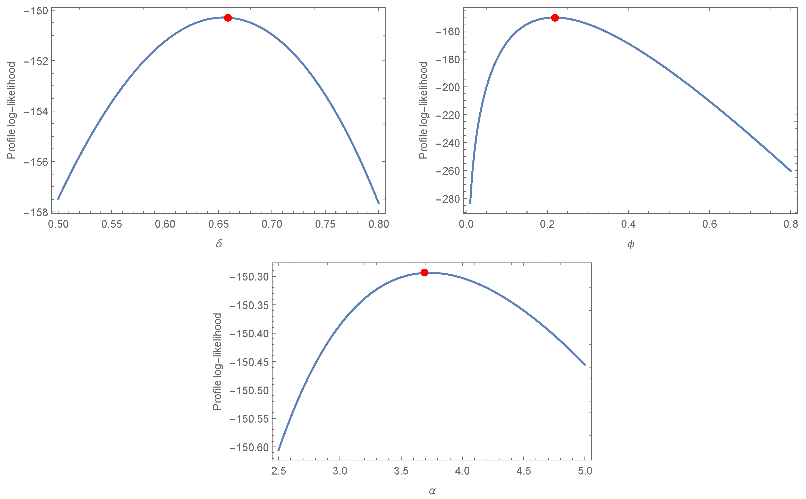
As we can see, the expressions of the MLEs of the NACos-Weibull distribution are not explicit forms. Therefore, we can implement the Newton–Raphson iteration method to obtain the exact value of the MLEs. In order to show the uniqueness of the MLEs, we plot the profiles of the log-likelihood functions of δ ^ M L E , ϕ ^ M L E , and α ^ M L E ; see Figure 3, Figure 4 and Figure 5. Using the hydrological data set (see Section 5), the plots in Figure 3 confirm the uniqueness of δ ^ M L E , ϕ ^ M L E , and α ^ M L E , whereas using the first and second engineering data sets (see Section 5), the plots in Figure 4 and Figure 5 confirm the uniqueness of δ ^ M L E , ϕ ^ M L E , and α ^ M L E , respectively.

4.2. Simulation

In this subsection, we accomplish the second aim that is concerned with the evaluation of δ ^ M L E , ϕ ^ M L E ,  and α ^ M L E through a brief simulation study (SS).
The SS of the NACos-Weibull distribution is carried out by choosing random samples, say n = 25 , 50 , , 1000 . These samples are obtained using the inverse CDF (also known as quantile function) given by
Q u = 1 ϕ log 2 π cos 1 Δ 1 / δ ,
where Δ is defined in Section 3.
The SS is conducted for three different combination of δ , ϕ , and α . These combination values are given by (i) δ = 0.7 , ϕ = 1.0 , α = 1.2 , (ii) δ = 0.6 , ϕ = 1.0 , α = 1.4 , and (iii) δ = 0.7 , ϕ = 1.2 , α = 1.5 .
The judgement about the performances of the δ ^ M L E , ϕ ^ M L E ,  and α ^ M L E are made by considering two evaluation criteria. These criteria are given by
  • Mean square error (MSE)
    M S E δ ^ M L E = 1 1000 i = 1 1000 δ ^ i δ 2 .
  • Bias
    B i a s δ ^ M L E = 1 1000 i = 1 1000 δ ^ i δ .
The above evaluation criteria are also computed for ϕ ^ M L E and α ^ M L E .
The SS is performed using the optim ( ) R -function with argument method = L - BFGS - B . The simulation code is also provided in the Appendix A. After performing the SS, the obtained results are presented numerically (see Table 1, Table 2 and Table 3) and visually (see Figure 6, Figure 7 and Figure 8). From the results of the SS of the NACos-Weibull distribution presented in Table 1, Table 2 and Table 3 and Figure 6, Figure 7 and Figure 8, we can see that
  • As n increases (i.e., as n ), the values of δ ^ M L E , ϕ ^ M L E , and α ^ M L E tend to become stable.
  • As n , the MSEs of δ ^ M L E , ϕ ^ M L E , and α ^ M L E decay to zero.
  • As n , the Biases of δ ^ M L E , ϕ ^ M L E , and α ^ M L E tend toward zero.
Table 1. The numerical illustration of the SS of the NACos-Weibull distribution for δ = 0.7 , ϕ = 1.0 , and α = 1.2 .
nParametersMLEsMSEsBiases
δ 0.71790.01610.0179
25 ϕ 1.11790.07610.1179
α 1.99272.80290.7927
δ 0.70200.00820.0020
50 ϕ 1.06870.03820.0687
α 1.88722.45420.6872
δ 0.69680.0054−0.0031
75 ϕ 1.05710.02770.0571
α 1.84432.27570.6443
δ 0.69270.0045−0.0072
100 ϕ 1.05420.02490.0542
α 1.77742.03460.5774
δ 0.69390.0027−0.0060
200 ϕ 1.03630.01620.0363
α 1.65111.58510.4511
δ 0.69780.0012−0.0021
400 ϕ 1.01320.00700.0132
α 1.38830.66740.1883
δ 0.69830.0007−0.0016
600 ϕ 1.00930.00510.0093
α 1.34560.48510.1456
δ 0.70160.00040.0016
800 ϕ 1.00130.00250.0013
α 1.23620.16960.0362
δ 0.70090.00020.0009
1000 ϕ 1.00020.00170.0002
α 1.22670.11660.0267
Table 2. The numerical illustration of the SS of the NACos-Weibull distribution for δ = 0.6 , ϕ = 1.0 , and α = 1.4 .
nParametersMLEsMSEsBiases
δ 0.63130.01390.0313
25 ϕ 1.07300.06610.0730
α 1.92762.33470.5276
δ 0.61740.00660.0174
50 ϕ 1.03800.03370.0380
α 1.85152.00220.4515
δ 0.60880.00380.0088
75 ϕ 1.01570.02230.0157
α 1.77711.80680.3771
δ 0.60420.00320.0042
100 ϕ 1.02610.02050.0261
α 1.79701.68470.3970
δ 0.60620.00160.0062
200 ϕ 1.00360.00990.0036
α 1.58940.98110.1894
δ 0.60340.00020.0034
800 ϕ 0.99350.0014−0.0064
α 1.38480.1150−0.0151
δ 0.60290.00010.0029
1000 ϕ 0.99400.0007−0.0059
α 1.39150.0422−0.0284
δ 0.60480.00070.0048
400 ϕ 0.99500.0048−0.0049
α 1.44650.42700.0465
δ 0.60540.00030.0054
600 ϕ 0.99050.0021−0.0094
α 1.36390.1265−0.0360
Table 3. The numerical illustration of the SS of the NACos-Weibull distribution for δ = 0.7 , ϕ = 1.2 , and α = 1.5 .
nParametersMLEsMSEsBiases
δ 0.73900.02090.0390
25 ϕ 1.28890.09710.0889
α 2.06372.63660.5637
δ 0.71690.00980.0169
50 ϕ 1.24980.04910.0498
α 2.03152.45950.5315
δ 0.71190.00620.0119
75 ϕ 1.22370.03300.0237
α 1.94222.16150.4422
δ 0.70400.00470.0040
100 ϕ 1.23480.02970.0348
α 2.01972.27860.5197
δ 0.70070.00310.0007
200 ϕ 1.21930.01810.0193
α 1.91121.80010.4112
δ 0.70500.00140.0050
400 ϕ 1.19930.0091−0.0006
α 1.63010.80880.1301
δ 0.70640.00090.0064
600 ϕ 1.18800.0054−0.0119
α 1.50420.41000.0042
δ 0.70440.00060.0044
800 ϕ 1.19110.0035−0.0088
α 1.49670.2741−0.0032
δ 0.70470.00040.0047
1000 ϕ 1.19150.0026−0.0084
α 1.49940.1718−0.0205
Figure 6. The visual illustration of the SS of the NACos-Weibull distribution for δ = 0.7 , ϕ = 1.0 , and α = 1.2 .
Mathematics 11 00673 g006
Figure 7. The visual illustration of the SS of the NACos-Weibull distribution for δ = 0.6 , ϕ = 1.0 , and α = 1.4 .
Mathematics 11 00673 g007
Figure 8. The visual illustration of the SS of the NACos-Weibull distribution for δ = 0.7 , ϕ = 1.2 , and α = 1.5 .
Mathematics 11 00673 g008

5. Applications Using the Hydrological and Engineering Data Sets

This section offers the illustration and applicability of the NACos-Weibull distribution. These facts are shown by taking three data sets from the hydrological and engineering sectors.
Using the hydrological and engineering data sets, we compare the results of the NACos-Weibull model with four other different well-known variants of the Wei model, namely the (i) logarithmic Weibull (for short, “L-Weibull”) distribution, (ii) new exponential cosine Weibull (for short, “NEC-Weibull”) distribution, (iii) new exponential Weibull (for short, “NE-Weibull”) distribution, and (iv) exponentiated Weibull (for short, “E-Weibull”), distribution.
The distribution functions of the above competing models are respectively expressed by
G x ; β , η , ψ = 1 1 η 1 e ϕ x δ η log 1 e ϕ x δ β , x 0 , β , η > 0 ,
G x ; η , ψ = 1 cos π 2 1 e ϕ x δ 1 1 η e ϕ x δ , x 0 , η > 0 ,
G x ; θ , ψ = 1 1 1 e ϕ x δ θ e 1 e ϕ x δ θ , x 0 , θ > 0 ,
and
G x ; θ , ψ = 1 e ϕ x δ θ , x 0 , θ > 0 .
To carry out the comparison of the NACos-Weibull and other above-mentioned models (i.e., competing distributions), we consider different selection criteria. These criteria are taken with the aim to figure out the most suitable model for the hydrological and engineering data sets. The selection criteria are given by
  • The Anderson Darling (represented by AD) test
    The AD test is a statistical quantity used to show the fitting power of a particular probability model for the underline data set. The main work of the AD test is to show if a considered sample of data is taken from the target population using a specific statistical model. The AD test can also be considered as an alternative test to the χ 2 test and computed as
    A D = n w ,
    where w is given by 1 n j = 1 n log G x j + log 1 G x n j + 1 2 j 1 .
  • The Cramer-Von-Messes (denoted by CVM) test
    The CVM test is another useful evaluating criterion for comparing the fitting power (or fitting results) of two or more probability models. A probability model with the lowest value of the CVM criterion is preferred. The numerical value of the CVM test is obtained as
    1 n j = 1 k log 1 G x n j + 1 + log G x j 2 j 1 n .
  • The Kolmogorov–Smirnov (expressed by KS) test
    Another criterion that we considered for comparing the NACos-Weibull and other competing models is the KS test. Let G n x and G ^ x represent the fitted CDF (i.e., CDF of the selected model) and empirical CDF, respectively. Then, the value of the KS criterion is computed as
    s u p x G k x G ^ x .
  • Akaike information criterion (AIC) The Akaike information criterion (AIC) is another decisive tool for checking how well a particular probability model fits the underlined data set. Let k represent the number of parameters of a model and represent the corresponding LLF of the model; then, the value of AIC is obtained as
    2 k 2 .
In addition to the above-selected criteria, we also consider the p-value for comparative purposes. For a particular data set, a probability model with smaller values of AIC, AD, CVM, KS, and the highest p-value is termed as the best suitable probability model.
The numerical values of the AD, CVM, and KS tests along with p-value are computed with the help of computer software called R - package using the SANN method.

5.1. Analysis of the Hydrological Data Set

Here, we apply the NACos-Weibull distribution using the hydrological data set. This data set consists of seventy-three observations and represents the exceedances of the flood peaks measured in m 3 / s e c . This data set was recorded at the Wheaton River, which is situated near Carcross in Yukon Territory, Canada. This data set has also been analyzed by numerous authors; see Bourguignon et al. [18], Merovci and Puka [19], and Hameldarbandi and Yilmaz [20].
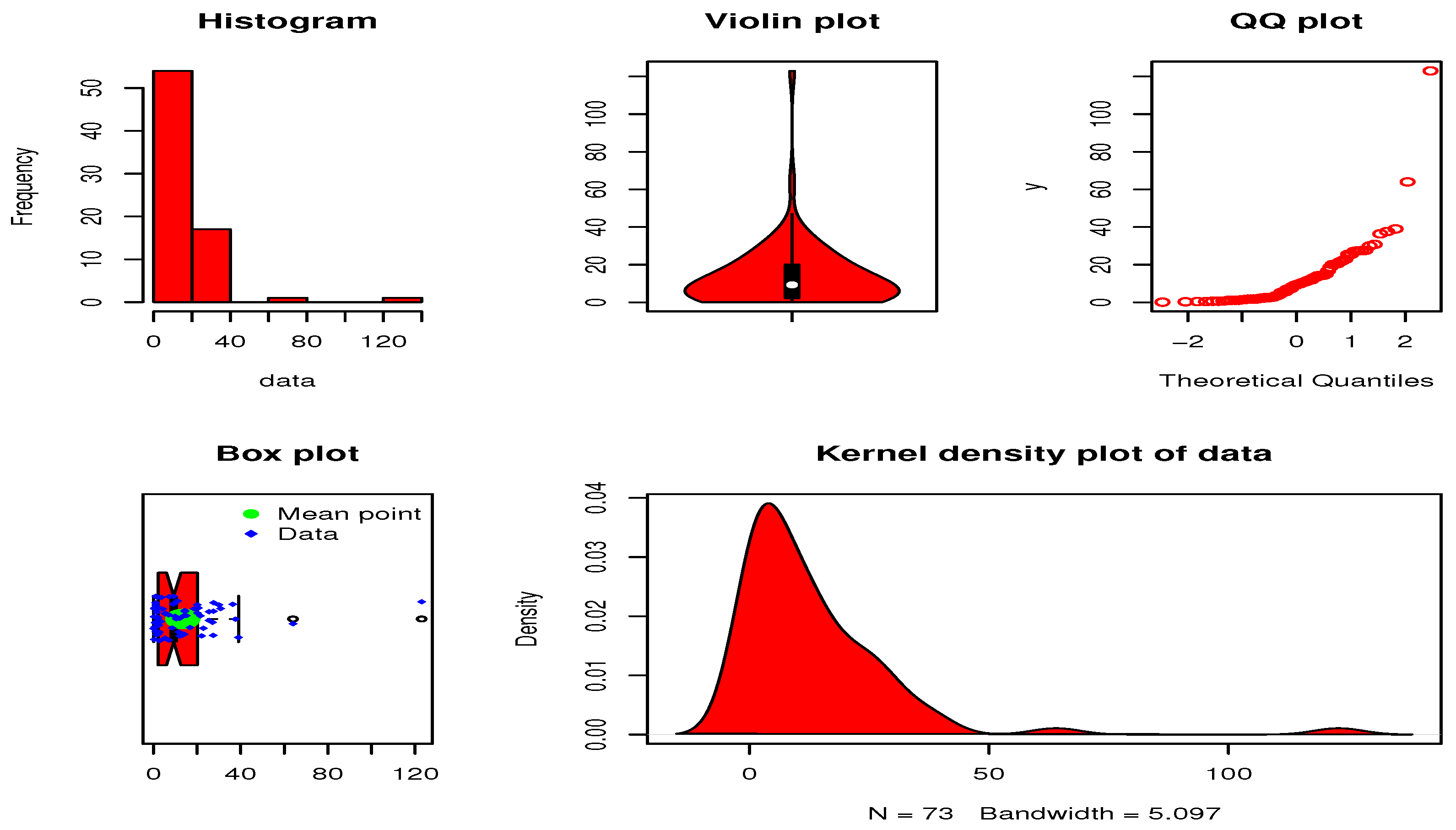
The flood peaks data set along with its some key summary measures are presented in Table 4. Corresponding to this data set, some basic description plots are presented in Figure 9.
After performing the numerical analysis, the values of δ ^ M L E , ϕ ^ M L E , α ^ M L E , θ ^ M L E , β ^ M L E , and η ^ M L E are presented in Table 5. The values of AIC, AD, CVM, and KS tests with p-value of the fitted models are provided in Table 6.
From Table 6, it can be seen that based on the AIC, AD, CVM, and KS tests with p-value, the proposed NACos-Weibull is the best probability model for analyzing the flood peaks data set because the values of the selected statistical tools (i.e., AD, KS, CVM, and AIC) for the NACos-Weibull distribution are smaller and have high p-value.
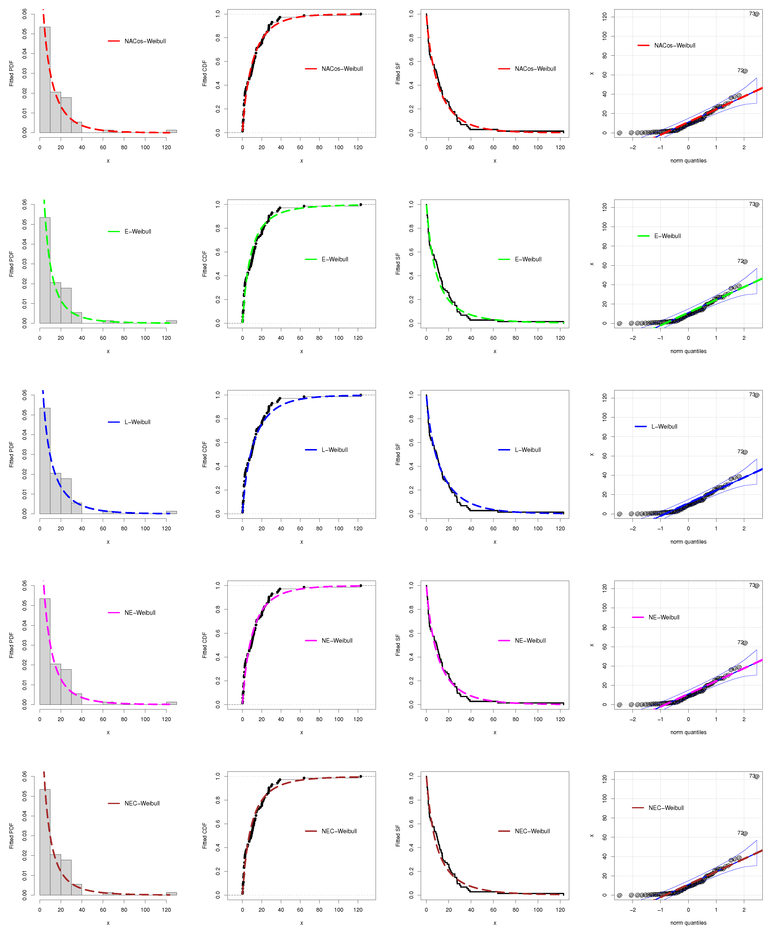
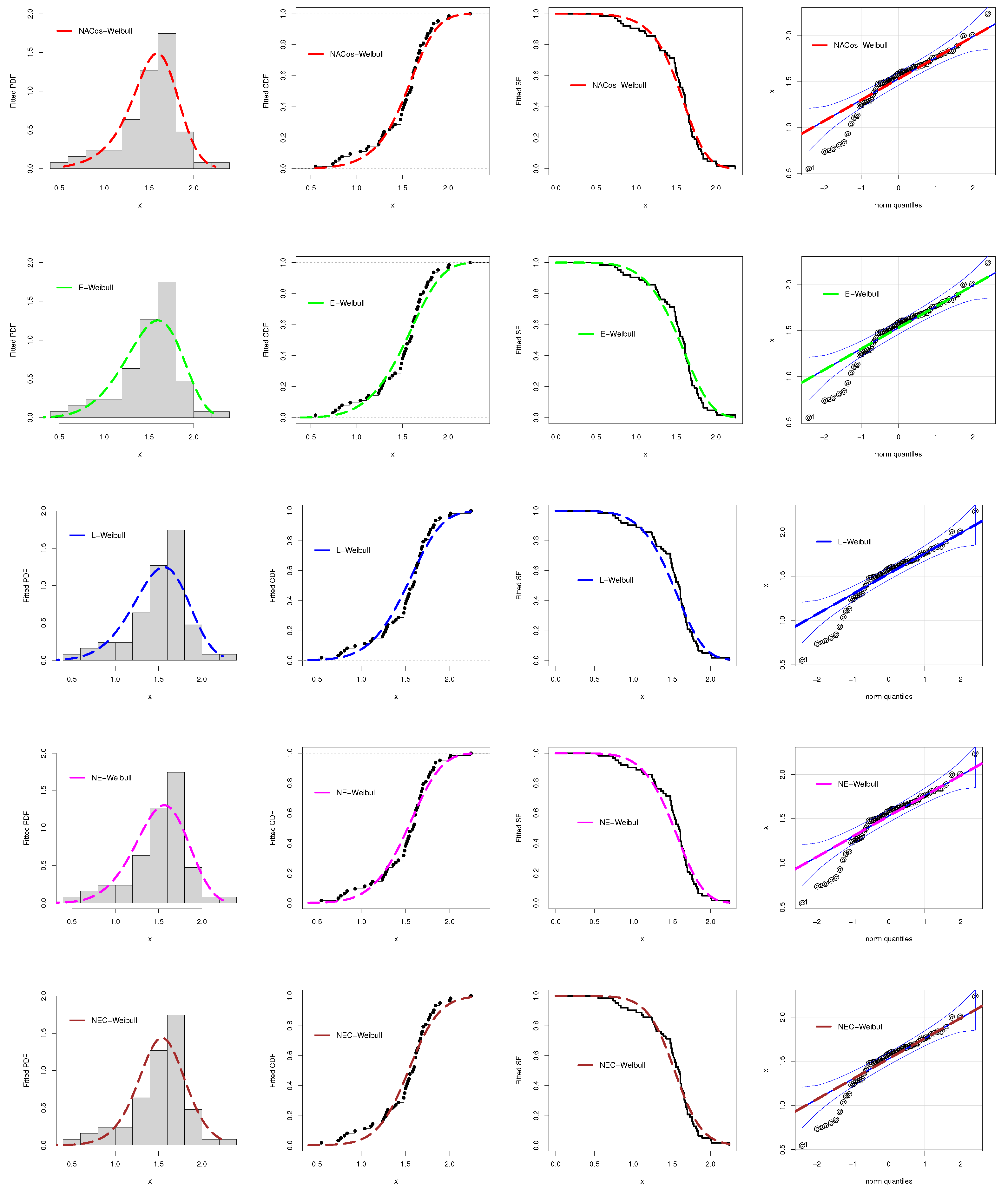
After the numerical comparison of the NACos-Weibull distribution and other variants of the Wei distribution in Table 6, we also provide a visual comparison of these fitted models. For the visual comparison, we select the plots of the fitted PDF, SF, quantile-quantile (QQ), and estimated CDF (see Figure 10). The plots in Figure 10 illustrate that the NACos-Weibull distribution closely follows the estimated SF, CDF, and PDF.

5.2. Analysis of the Engineering Data Sets

In this subsection, we analyze the engineering data sets to illustrate the applicability of the NACos-Weibull distribution in the engineering sector. The first engineering data set represents the failure times of electronic items, whereas the second engineering data set represents the strengths of glass fibers.

5.2.1. The Failure Times Data

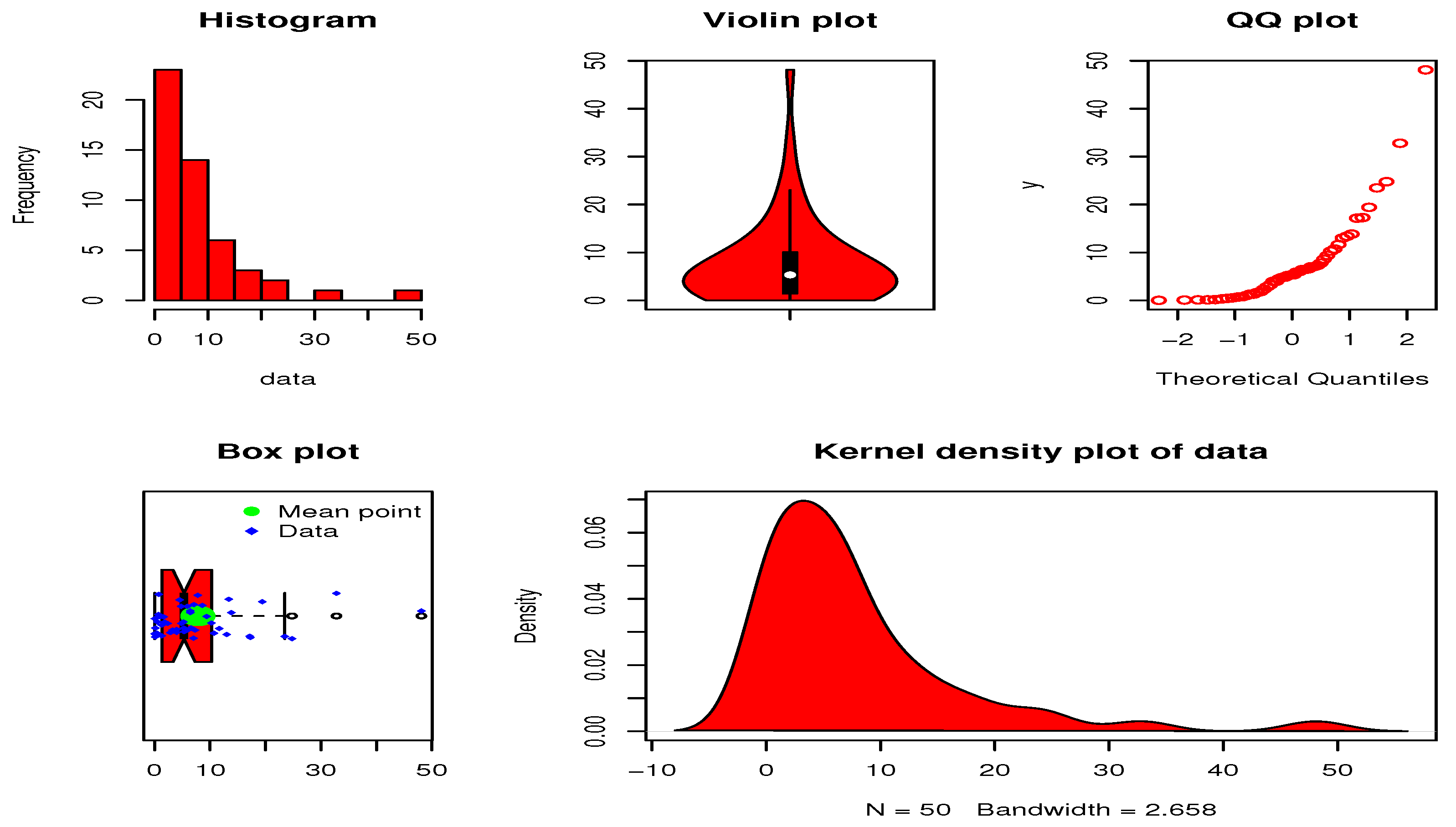
Here, we provide the second practical illustration of the NACos-Weibull model by analyzing the engineering data set. This data set consists of fifty observations and represents the failure times of electronic items measured in weeks (see Murthy et al. [21]). The failure times data set along with its some key summary measures are provided in Table 7. Furthermore, some basic description plots of this data set are also presented in Figure 11.
Corresponding to the failure times data, the values of δ ^ M L E , ϕ ^ M L E , α ^ M L E , θ ^ M L E , β ^ M L E , and η ^ M L E of the fitted distributions are presented in Table 8, whereas the values of the AIC, AD, CVM, and KS tests with the p-value of the fitted competing models are provided in Table 9.
From Table 8, it is obvious that the NACos-Weibull distribution has the smallest values of the statistical measures and a high p-value. Thus, we conclude that using the failure times data, the NACos-Weibull again performs better as compared to the other fitted distributions.
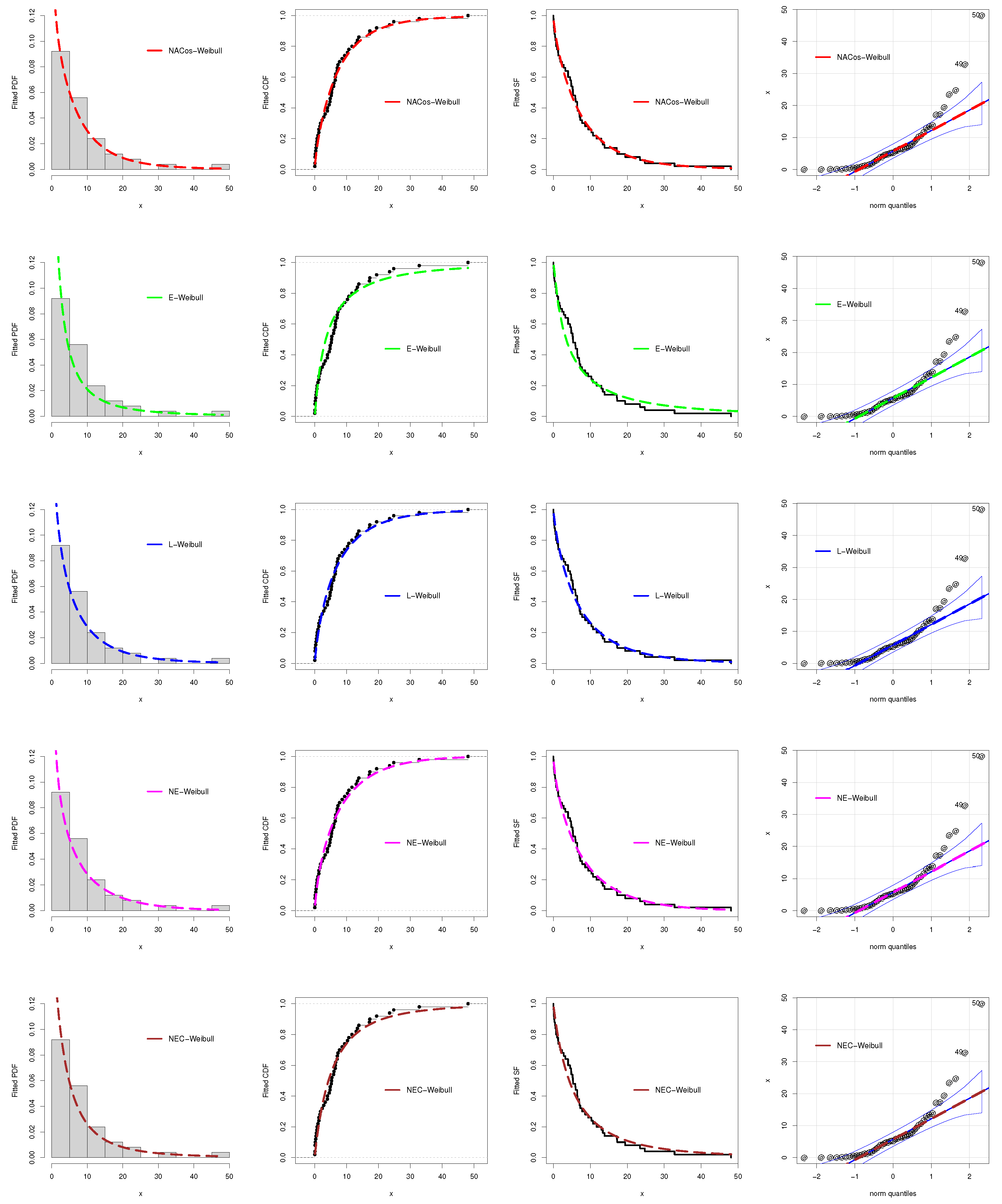
Besides the numerical comparison of the NACos-Weibull distribution and other competing distributions in Table 9, we also provide a visual comparison of these fitted probability models. For the visual comparison, we again selected the plots of the fitted PDF, CDF, QQ, and SF. The plots in Figure 12 also confirm the best-/close-fitting capability of the NACos-Weibull distribution.

5.2.2. The Glass Fibers Data

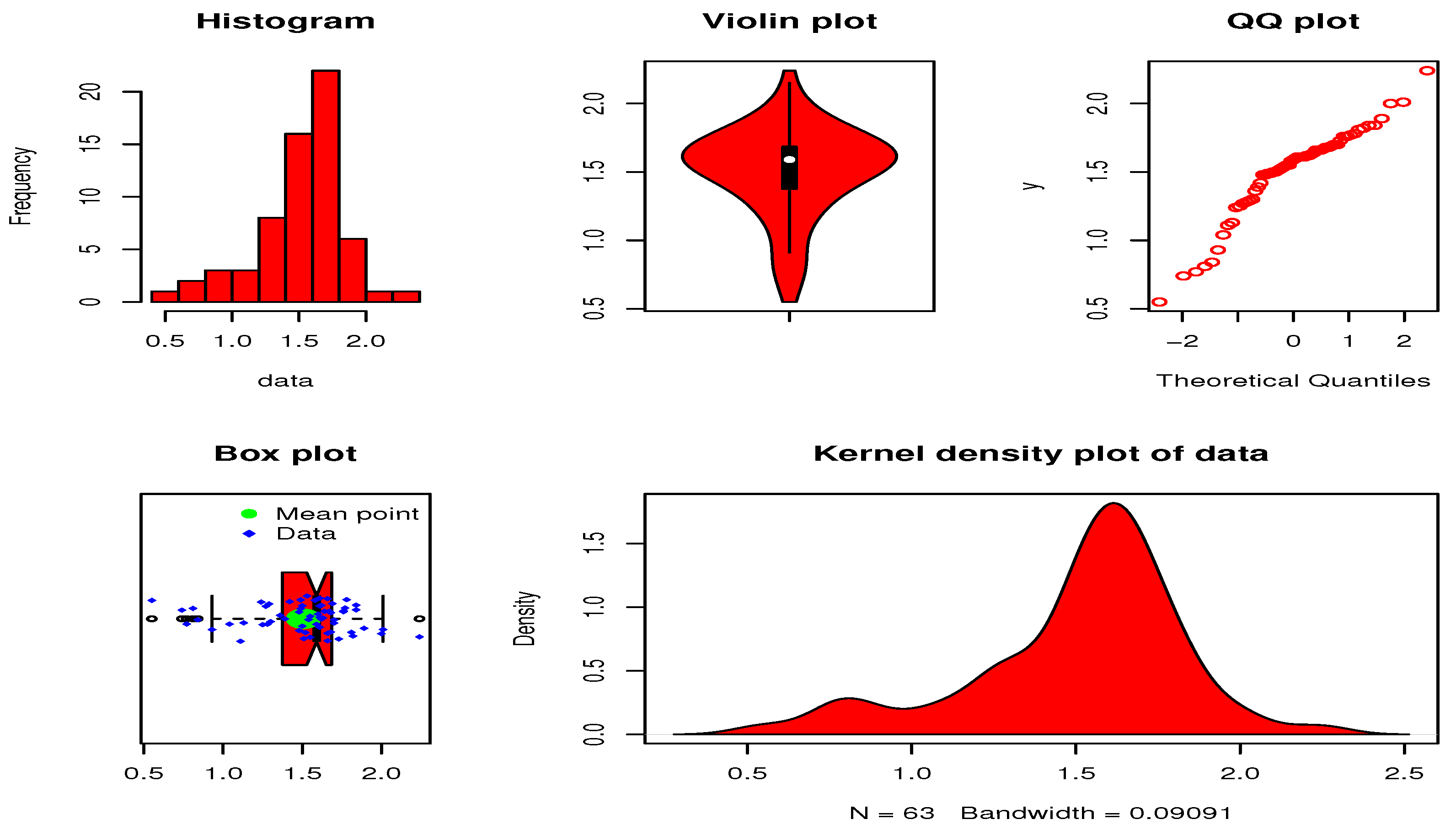
Here, we provide the third practical illustration of the NACos-Weibull model by analyzing another engineering data set. This data set consists of sixty-three observations and represents the strengths of 1.5 cm glass fibers (see Smith and Naylor [22]). The glass fibers data set along with its some key summary measures are presented in Table 10. Corresponding to the glass fibers data, some description plots are also presented in Figure 13.
Corresponding to the glass fibers data, the values of δ ^ M L E , ϕ ^ M L E , α ^ M L E , θ ^ M L E , β ^ M L E , and η ^ M L E of the fitted distributions are reported in Table 11, whereas the values of the statistical criteria of the fitted competing models are reported in Table 12.
Based on the given results in Table 12, it is clear that the NACos-Weibull distribution has again the smallest values of the statistical criteria and a high p-value. Therefore, we conclude that using the glass fibers data, the NACos-Weibull again outperforms the other fitted models.
In addition to the numerical comparison of the NACos-Weibull distribution and other fitted distributions presented in Table 12, we also provide a visual comparison of these fitted competing models. For this activity, we again consider the plots of the fitted PDF, CDF, QQ, and SF. Based on the visual comparisons in Figure 14, it is clear that the NACos-Weibull distribution fits the glass fibers data closely.

6. Conclusions

A new probability model, based on the Weibull distribution and trigonometric function, has been proposed and its different distributional properties are studied. The idea was to utilize the cosine function to obtain a new updated version of the Weibull distribution, namely a NACos-Weibull distribution. The MLEs of the NACos-Weibull distribution are derived. Furthermore, a SS was also conducted to see the behavior of the MLEs of the NACos-Weibull distribution. Finally, we showed the applicability of the NACos-Weibull distribution using three data sets. The first data set was considered from the hydrological sector, whereas the second and third data sets were taken from the engineering sector. The comparisons of the NACos-Weibull distribution were made with four well-known variants (i.e., E-Weibull, L-Weibull, NE-Weibull, and NEC-Weibull) of the Weibull distribution. Based on certain statistical criteria such as AIC, AD, KS, CVM, and p-value, we observed that the NACos-Weibull distribution was repeatedly the best competing model for the hydrological and engineering data sets.
Future work includes reduction of the parameters, bivariate extension, regression problems with covariates, acceptance sampling plane, and applications in quality control.

Author Contributions

A.S.A. was responsible for Conceptualization, methodology, investigation, writing and M.M.A.E.-R. was responsible for resources, writing, visualization. All authors have read and agreed to the published version of the manuscript.

Funding

This research received no external funding.

Data Availability Statement

All data available in the paper.

Acknowledgments

This research work was funded by Institutional Fund Projects under grant no. (IFPIP: 228-662-1443). The authors gratefully acknowledge technical and financial support provided by the Ministry of Education and King Abdulaziz University, DSR, Jeddah, Saudi Arabia.

Conflicts of Interest

The authors have no conflict of interest.

Appendix A. R Code for Simulation Study

remove(list=ls())
library(rootSolve)
library(AdequacyModel)
#################### Genertng Random Sample
rNew_Weibull=function(par,n)
{
del=par[1]; phi=par[2]; a=par[3]
u=runif(n)
x=c()
for (i in 1:n)
{
f = function(x)
((a^(cos((pi/2)-(pi/2)*(1-exp(-phi*x^(del)))))-1)/(a-1))-u[i]
#################### Loading package rootSolve
x[i] = rootSolve::uniroot.all(f , interval = c(0,100000))
}
return(x)
}
#################### PDF
dNew_Weibull <- function(par,x)
{
del= par[1]
phi= par[2]
a = par[3]
(pi*(log(a))*del*phi*(x^(del-1))*exp(-phi*x^(del))*
sin((pi/2)-(pi/2)*(1-exp(-phi*x^(del))))*
a^(cos((pi/2)-(pi/2)*(1-exp(-phi*x^(del)))))/(2*(a-1)))
}
#################### CDF
pNew_Weibull<- function(par,x)
{
del= par[1]
phi= par[2]
a = par[3]
((a^(cos((pi/2)-(pi/2)*(1-exp(-phi*x^(del)))))-1)/(a-1))
}
#################### Loglikelihood function
loglikelihoodNew_Weibull <- function(par){
del= par[1]
phi= par[2]
a = par[3]
aux = sin((pi/2)-(pi/2)*(1-exp(-phi*x^(del))))
aux1 = a^(cos((pi/2)-(pi/2)*(1-exp(-phi*x^(del)))))
if(del>0 && phi>0 && a>0 && min(x)>0 && min(aux)>0 && min(aux1)>0)
{
w = log(pi)+log(log(a))+log(del)+log(phi)+(del-1)*log(x)-(phi*x^del)
+log(aux)+log(aux1)-log(2*(a-1))
 return(sum(w))
}else{
return(-9999999.9)
}
}
#################### Function for simulation study
par <- c(0.7, 1, 1.2); del=0.7; phi=1; a=1.2
n_replicas = 1000
matriz_par <- matrix(0,40,3)
matriz_bias<- matrix(0,40,3)
matriz_MSE <- matrix(0,40,3)
matriz_std <- matrix(0,40,3)
 
colnames(matriz_par) <- c("del", "phi", "a")
colnames(matriz_bias)<- c("del", "phi", "a")
colnames(matriz_MSE) <- c("del", "phi", "a")
colnames(matriz_std) <- c("del", "phi", "a")
 
cont = 1
n = 25
while(n <= 1000){
par_mean <- c(0,0,0)
std_mean <- c(0,0,0)
bias <- c(0,0,0)
MSE <- c(0,0,0)
 
replica = 1
while(replica <= n_replicas){
print(paste("n = ",n, ", replica = ", replica) )
x <- rNew_Weibull(par,n)
Data <- x
####################
result=optim(c(del, phi,a), loglikelihoodNew_Weibull, hessian = F,
control = list(fnscale = -1), method = "L-BFGS-B",
lower = c(0.001, 0.001, 1.001), upper = c(5,5,5))
if (class(result) != "try-error" && result$convergence == 0){
par_mean <- par_mean + result$par
bias = bias + (result$par - par)
MSE = MSE + (result$par - par)^2
replica = replica +1
}
}
 
par_mean = par_mean/n_replicas
bias = bias/n_replicas
MSE = MSE/n_replicas
 
matriz_par[cont,] = par_mean
matriz_std[cont,] = std_mean
matriz_bias[cont,] = bias
matriz_MSE[cont,] = MSE
 
print("mean = ")
print( par_mean )
print("bias = ")
print( bias )
print("MSE = ")
print( MSE )
n = n + 25
cont = cont +1
}
print(matriz_par)
print(matriz_MSE)
print(matriz_bias)
n=seq(25, 1000, 25)
####################
plot(n,(matriz_par[,1]), type="o", col="green", lty=1, lwd=3,xlab="n",
 ylab="Estimated parameters",ylim=c(0.1,3.5))
lines(n,(matriz_par[,2]), col="blue", lty=5,lwd=3,type="o")
lines(n,(matriz_par[,3]), col="red", lty=8,lwd=3,type="o")
legend(500,3.2, legend = c(expression(paste(delta," = ","0.7")),
                           expression(paste(phi," = ","1.0")),
        expression(paste(alpha," = ","1.2"))),
lty =c(1,5,8),cex=1.2, col=c(’green’,’blue’,’red’),box.lty=0)
####################
 plot(n,matriz_MSE[,1], col="green", lty=1, lwd=3,type="o", xlab="n",
 ylab="MSE", ylim=c(0,3.5))
 lines(n,matriz_MSE[,2], col="blue", lty=5, lwd=3,type="o")
 lines(n,matriz_MSE[,3], col="red", lty=8,lwd=3,type="o")
legend(500,3.2, legend = c(expression(paste(delta," = ","0.7")),
                           expression(paste(phi," = ","1.0")),
        expression(paste(alpha," = ","1.2"))),
lty =c(1,5,8),cex=1.2, col=c(’green’,’blue’,’red’),box.lty=0)
####################
plot(n,(matriz_bias[,1]), type="o", col="green", lty=1, lwd=3, xlab="n",
ylab="Bias",ylim=c(-0.09,1))
 lines(n,(matriz_bias[,2]), col="blue", lty=5,lwd=3,type="o")
 lines(n,(matriz_bias[,3]), col="red", lty=8, lwd=3,type="o")
legend(500,0.9, legend = c(expression(paste(delta," = ","0.7")),
                           expression(paste(phi," = ","1.0")),
        expression(paste(alpha," = ","1.2"))),
lty =c(1,5,8),cex=1.2, col=c(’green’,’blue’,’red’),box.lty=0)

References

  1. Silahli, B.; Dingec, K.D.; Cifter, A.; Aydin, N. Portfolio value-at-risk with two-sided Weibull distribution: Evidence from cryptocurrency markets. Financ. Res. Lett. 2021, 38, 101425. [Google Scholar] [CrossRef]
  2. Teamah, A.E.A.; Elbanna, A.A.; Gemeay, A.M. Heavy-tailed log-logistic distribution: Properties, risk measures and applications. Stat. Optim. Inf. Comput. 2021, 9, 910–941. [Google Scholar] [CrossRef]
  3. Ahmad, Z.; Mahmoudi, E.; Dey, S. A new family of heavy tailed distributions with an application to the heavy tailed insurance loss data. Commun. Stat.-Simul. Comput. 2022, 51, 4372–4395. [Google Scholar] [CrossRef]
  4. Chaito, T.; Khamkong, M. The Length–Biased Weibull–Rayleigh Distribution for Application to Hydrological Data. Lobachevskii J. Math. 2021, 42, 3253–3265. [Google Scholar] [CrossRef]
  5. Shahmari, M.; Zarafshan, P.; Kouravand, S.; Khashehchi, M. Design and analysis of a combined savonius-darrieus wind turbine for irrigation application. J. Renew. Energy Environ. 2020, 7, 80–86. [Google Scholar]
  6. Suwarno, S.; Zambak, M.F. The Probability Density Function for Wind Speed Using Modified Weibull Distribution. Int. J. Energy Econ. Policy 2021, 11, 544. [Google Scholar] [CrossRef]
  7. Al-Babtain, A.A.; Elbatal, I.; Al-Mofleh, H.; Gemeay, A.M.; Afify, A.Z.; Sarg, A.M. The Flexible Burr XG Family: Properties, Inference, and Applications in the Engineering Science. Symmetry 2021, 13, 474. [Google Scholar] [CrossRef]
  8. Strzelecki, P. Determination of fatigue life for low probability of failure for different stress levels using 3-parameter Weibull distribution. Int. J. Fatigue 2021, 145, 106080. [Google Scholar] [CrossRef]
  9. Sindhu, T.N.; Atangana, A. Reliability analysis incorporating exponentiated inverse Weibull distribution and inverse power law. Qual. Reliab. Eng. Int. 2021, 37, 2399–2422. [Google Scholar] [CrossRef]
  10. Abubakar, H.; Muhammad Sabri, S.R. A Simulation Study on Modified Weibull Distribution for Modelling of Investment Return. Pertanika J. Sci. Technol. 2021, 29. [Google Scholar] [CrossRef]
  11. Kovacs, K.; Ansari, F.; Sihn, W. A modified Weibull model for service life prediction and spare parts forecast in heat treatment industry. Procedia Manuf. 2021, 54, 172–177. [Google Scholar] [CrossRef]
  12. Liu, X.; Ahmad, Z.; Gemeay, A.M.; Abdulrahman, A.T.; Hafez, E.H.; Khalil, N. Modeling the survival times of the COVID-19 patients with a new statistical model: A case study from China. PLoS ONE 2021, 16, e0254999. [Google Scholar] [CrossRef]
  13. Dessalegn, Y.; Singh, B.; Vuure, A.W.V.; Badruddin, I.A.; Beri, H.; Hussien, M.; Hossain, N. Investigation of Bamboo Fibrous Tensile Strength Using Modified Weibull Distribution. Materials 2022, 15, 5016. [Google Scholar] [CrossRef] [PubMed]
  14. Alyami, S.A.; Elbatal, I.; Alotaibi, N.; Almetwally, E.M.; Okasha, H.M.; Elgarhy, M. Topp–Leone Modified Weibull Model: Theory and Applications to Medical and Engineering Data. Appl. Sci. 2022, 12, 10431. [Google Scholar] [CrossRef]
  15. Bakr, M.E.; Al-Babtain, A.A.; Mahmood, Z.; Aldallal, R.A.; Khosa, S.K.; Abd El-Raouf, M.M.; Hussam, E.; Gemeay, A.M. Statistical modelling for a new family of generalized distributions with real data applications. Math. Biosci. Eng. 2022, 19, 8705–8740. [Google Scholar] [CrossRef] [PubMed]
  16. Galton, F. Inquiries into Human Faculty and Its Development; Macmillan & Company: London, UK, 1883. [Google Scholar]
  17. Moors, J.J.A. A quantile alternative for kurtosis. J. R. Stat. Soc. Ser. D 1988, 37, 25–32. [Google Scholar] [CrossRef] [Green Version]
  18. Bourguignon, M.; Silva, R.B.; Zea, L.M.; Cordeiro, G.M. The Kumaraswamy Pareto distribution. J. Stat. Theory Appl. 2012, 12, 129–144. [Google Scholar] [CrossRef] [Green Version]
  19. Merovci, F.; Puka, L. Transmuted Pareto distribution. ProbStat Forum 2014, 7, 1–11. [Google Scholar]
  20. Hameldarbandi, M.; Yilmaz, M. A new perspective of transmuted distribution. Communications Faculty of Sciences University of Ankara Series A1. Math. Stat. 2019, 68, 1144–1162. [Google Scholar]
  21. Murthy, D.P.; Xie, M.; Jiang, R. Weibull Models; John Wiley & Sons: Hoboken, NJ, USA, 2004. [Google Scholar]
  22. Smith, R.L.; Naylor, J. A comparison of maximum likelihood and Bayesian estimators for the three-parameter Weibull distribution. J. R. Stat. Soc. Ser. C (Appl. Stat.) 1987, 36, 358–369. [Google Scholar] [CrossRef]
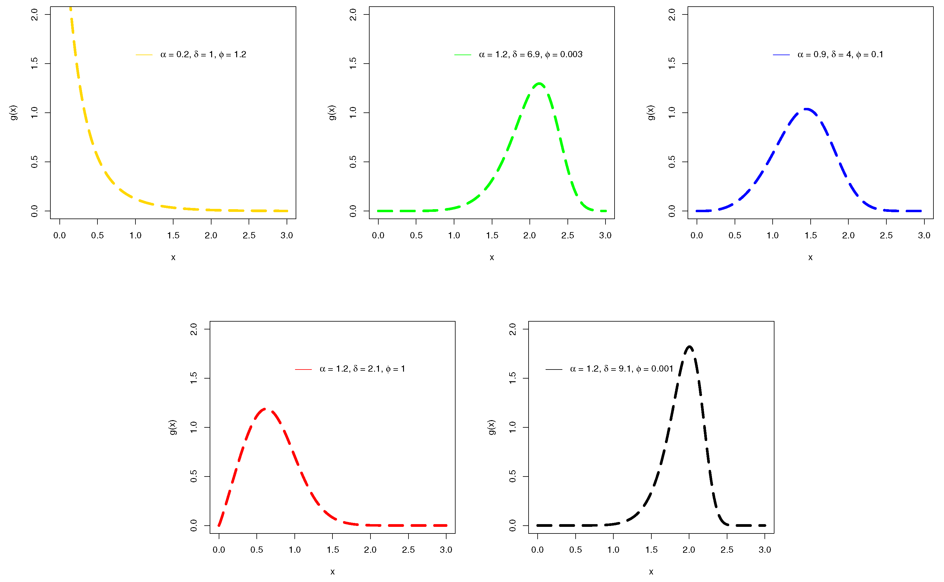
Figure 1. Illustrations of g x ; α , ψ of the NACos-Weibull for different values of α , ϕ , and δ .
Mathematics 11 00673 g001
Figure 2. Illustrations of h x ; α , ψ of the NACos-Weibull for different values of α , ϕ , and δ .
Mathematics 11 00673 g002
Figure 3. The profiles of the log-likelihood functions of δ ^ M L E , ϕ ^ M L E , and α ^ M L E using the hydrological data set.
Mathematics 11 00673 g003
Figure 4. The profiles of the log-likelihood functions of δ ^ M L E , ϕ ^ M L E , and α ^ M L E using the first engineering data set.
Mathematics 11 00673 g004
Figure 5. The profiles of the log-likelihood functions of δ ^ M L E , ϕ ^ M L E , and α ^ M L E using the second engineering data set.
Mathematics 11 00673 g005
Figure 9. Visual description of the flood peaks data set.
Mathematics 11 00673 g009
Figure 10. Using the flood peaks data set, the visual comparison of the fitted models.
Mathematics 11 00673 g010
Figure 11. Visual description of the failure times data set.
Mathematics 11 00673 g011
Figure 12. The visual comparison of the fitted models using the failure times data set.
Mathematics 11 00673 g012
Figure 13. Visual description of the glass fibers data set.
Mathematics 11 00673 g013
Figure 14. The visual comparison of the fitted models using the glass fibers data set.
Mathematics 11 00673 g014
Table 4. The flood peaks data set with summary values.
0.1, 0.3, 0.4, 0.4, 0.6, 0.6, 0.7, 1.0, 1.1, 1.1, 1.1, 1.4, 1.5, 1.7, 1.7, 1.7, 1.7, 1.9, 2.2,
2.2, 2.5, 2.5, 2.5, 2.7, 2.8, 3.4, 3.6, 4.2, 5.3, 5.3, 5.6, 7.0, 7.0, 7.3, 8.5, 9.0, 9.3, 9.7,
9.9, 10.4, 10.7, 11.0, 11.6, 11.9, 12.0, 13.0, 13.3, 14.1, 14.1, 14.4, 14.4, 15.0, 16.8,
18.7, 20.1, 20.2, 20.6, 21.5, 22.1, 22.9, 25.5, 25.5, 27.1, 27.4, 27.5, 27.6, 30.0, 30.8,
36.4, 37.6, 39.0, 64.0, 123.0.
nMin.Max. x ¯ Median V a r x
730.1000123.000013.45009.3000315.3845
Q 1 S D x Q 3 SkewnessKurtosisRange
2.200017.759020.10003.657721.6005122.9000
Table 5. Using the flood peaks data set, the values of δ ^ M L E , ϕ ^ M L E , α ^ M L E , θ ^ M L E ,   β ^ M L E , and η ^ M L E of the fitted distributions.
Models δ ^ MLE ϕ ^ MLE α ^ MLE θ ^ MLE β ^ MLE η ^ MLE
NACos-Weibull0.84320.05640.4754---
E-Weibull0.50150.5695-2.6997--
L-Weibull0.77440.8785--0.16163.2385
NE-Weibull0.95410.0517-0.9567--
NEC-Weibull0.58230.3609---1.0301
Table 6. For the flood peaks data set, the values of selection criteria of the fitted distributions.
ModelsAICCVMADKSp-Value
NACos-Weibull521.83110.08930.54560.08350.6888
E-Weibull526.99670.13520.73180.10560.3888
L-Weibull528.11780.09410.55560.10060.4500
NE-Weibull526.92490.10660.61650.08860.6147
NEC-Weibull526.97820.12880.70420.095990.5117
Table 7. The failure times data set with summary values.
0.013, 0.065, 0.111, 0.111, 0.163, 0.309, 0.426, 0.535, 0.684, 0.747, 0.997, 1.284, 1.304, 1.647,
1.829, 2.336, 2.838, 3.269, 3.977, 3.981, 4.520, 4.789, 4.849, 5.202, 5.291, 5.349, 5.911, 6.018,
6.427, 6.456, 6.572, 7.023, 7.087, 7.291, 7.787, 8.596, 9.388, 10.261, 10.713, 11.658, 13.006,
13.388, 13.842, 17.152, 17.283, 19.418, 23.471, 24.777, 32.795, 48.105
nMin.Max. x ¯ Median V a r x
500.013048.10507.82105.320084.7559
Q 1 S D x Q 3 SkewnessKurtosisRange
1.39009.206310.04302.30609.408248.0920
Table 8. Using the failure times data set, the values of δ ^ M L E , ϕ ^ M L E , α ^ M L E , θ ^ M L E , β ^ M L E , and η ^ M L E of the fitted distributions.
Models δ ^ MLE ϕ ^ MLE α ^ MLE θ ^ MLE β ^ MLE η ^ MLE
NACos-Weibull0.65860.21933.6914---
E-Weibull0.32941.3937-5.2871--
L-Weibull0.73530.1354--2.16524.8756
NE-Weibull1.53780.0090-0.4751--
NEC-Weibull0.41971.0590---3.0257
Table 9. For the failure times data set, the values of the selection criteria of the fitted distributions.
ModelsAICCVMADKSp-Value
NACos-Weibull302.58800.06190.31210.09560.7504
E-Weibull315.68840.23761.26240.17620.0896
L-Weibull309.53780.08640.43200.10620.6251
NE-Weibull306.78170.07250.36400.10650.6216
NEC-Weibull310.02370.13140.67650.11770.4923
Table 10. The glass fibers data set with summary values.
0.55, 0.93, 1.25, 1.36, 1.49, 1.52, 1.58, 1.61, 1.64, 1.68, 1.73, 1.81, 2, 0.74, 1.04, 1.27,
1.53, 1.59, 1.61, 1.66, 1.68, 1.76, 1.82, 2.01, 0.77, 1.11, 1.28, 1.42, 1.5, 1.54, 1.6, 1.62,
1.76, 1.84, 2.24, 0.81, 1.13, 1.29, 1.48, 1.5, 1.55, 1.61, 1.62, 1.66, 1.7, 1.77, 1.84, 0.84,
1.48, 1.51, 1.55, 1.61, 1.63, 1.67, 1.7, 1.78, 1.89 1.39, 1.49, 1.66, 1.69, 1.24, 1.3
nMin.Max. x ¯ Median V a r x
630.55002.24001.50701.59000.1050
Q 1 S D x Q 3 SkewnessKurtosisRange
1.37500.32411.6850−0.89993.923761.69
Table 11. Using the glass fibers data set, the values of δ ^ M L E , ϕ ^ M L E , α ^ M L E , θ ^ M L E , β ^ M L E , and η ^ M L E of the fitted distributions.
Models δ ^ MLE ϕ ^ MLE α ^ MLE θ ^ MLE β ^ MLE η ^ MLE
NACos-Weibull4.33750.11249.3757---
E-Weibull0.03960.8297-6.16298--
L-Weibull4.19490.1132--1.97011.2117
NE-Weibull1.53780.0090-0.4751--
NEC-Weibull2.71360.7702---5.3487
Table 12. For the glass fibers data set, the values of the selection criteria of the fitted distributions.
ModelsAICCVMADKSp-Value
NACos-Weibull32.44730.15850.87330.11910.3331
E-Weibull36.16570.22911.26130.14100.1632
L-Weibull38.44420.24231.32930.17000.0522
NE-Weibull36.78690.24781.36320.15570.0941
NEC-Weibull38.70780.28111.53980.13740.1846
Disclaimer/Publisher’s Note: The statements, opinions and data contained in all publications are solely those of the individual author(s) and contributor(s) and not of MDPI and/or the editor(s). MDPI and/or the editor(s) disclaim responsibility for any injury to people or property resulting from any ideas, methods, instructions or products referred to in the content.