
Micro-Thrust, Low-Fuel Consumption, and High-Precision East/West Station Keeping Control for GEO Satellites Based on Synovial Variable Structure Control


Abstract
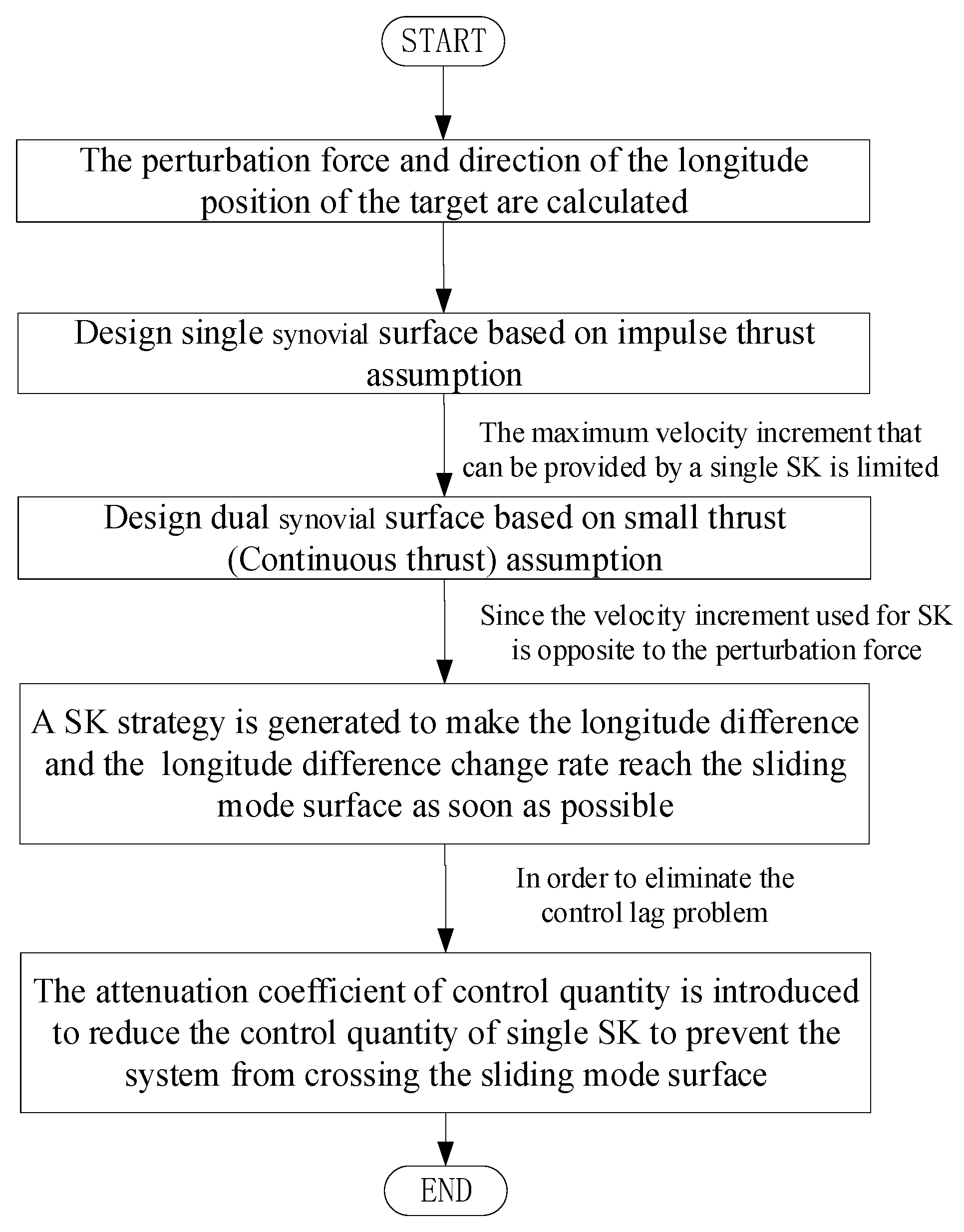
:1. Introduction
2. Mean Longitude Keeping Based on Single-Synovial Surface
- (1)
- The mean longitude keeping frequency is about once a day;
- (2)
- The thruster deviation angle is basically unchanged during the mean longitude keeping;
- (3)
- In order to achieve optimal fuel orbital capture and keeping, the velocity increment required for the mean longitude keeping is only used to overcome the orbital perturbation;
- (4)
- The longitude of the satellite satisfies the condition: ;
- (5)
- There is no constraint on the duration of capturing the target.
2.1. Mean Longitude Keeping Strategy
2.2. Calculation of Control Amount
2.3. Stability Analysis of Control Strategy
- (1)
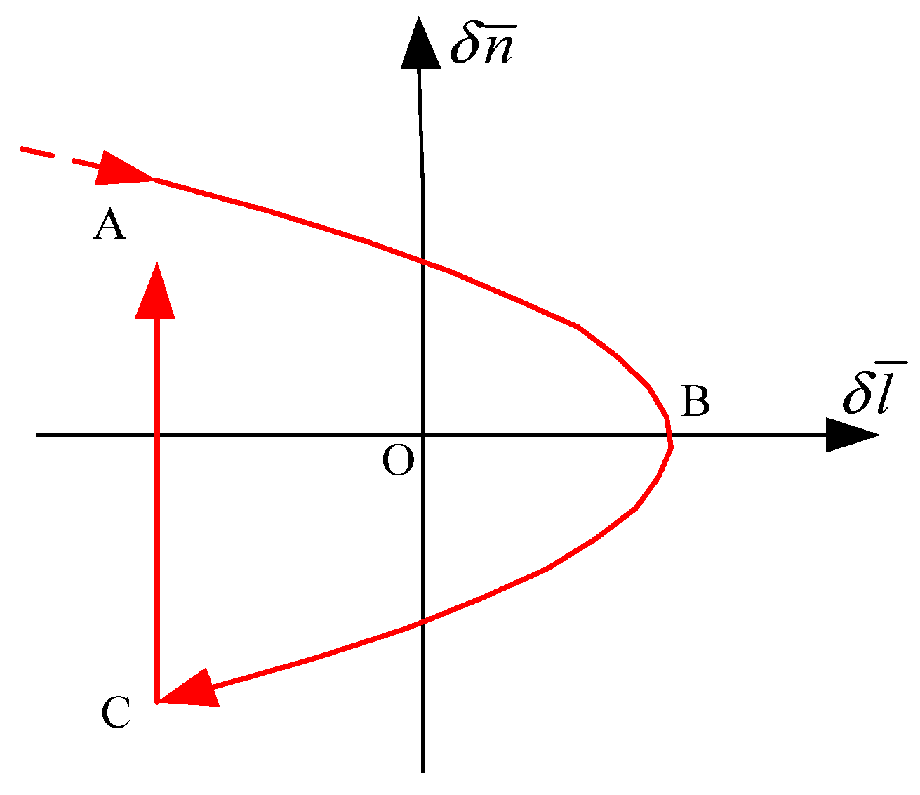
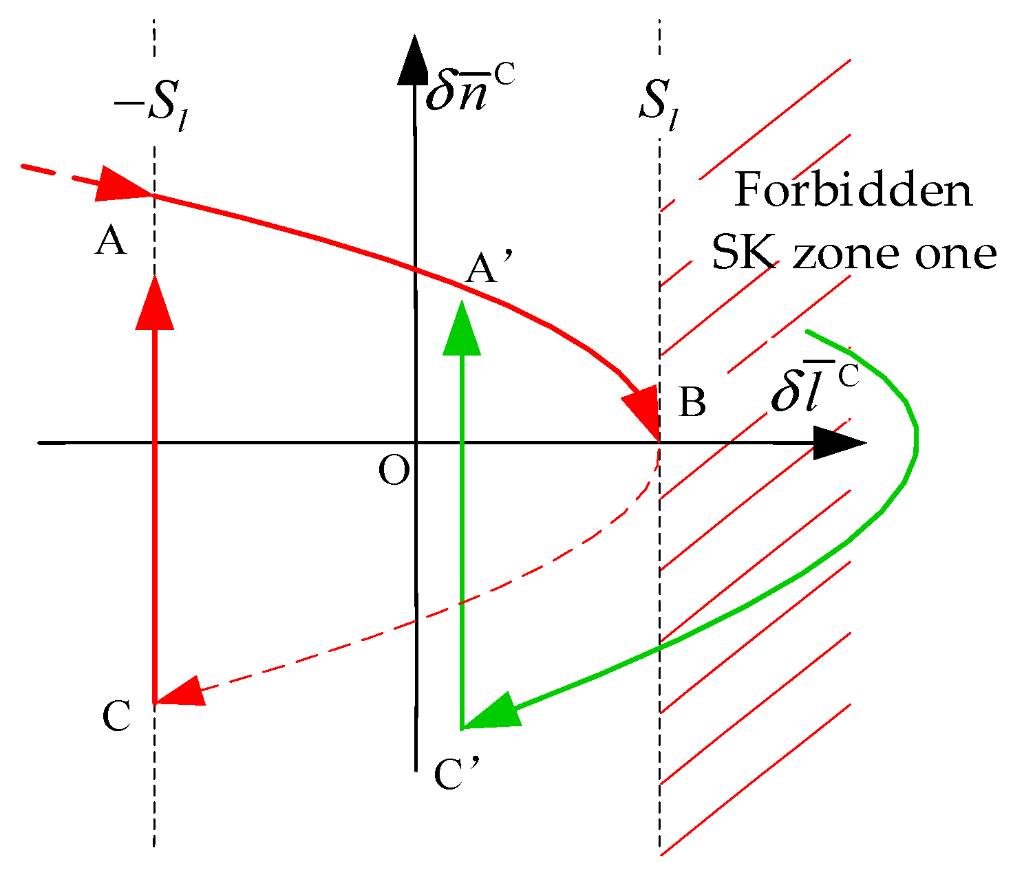
- As shown in Figure 4, when the initial mean longitude difference and the mean longitude drift rate is located at C’ (in the SK zone). Under the action of the tangential velocity increment, the mean longitude drift rate will change sign, and finally intersect with the synovial surface AB, and converge along the synovial surface AB to the vicinity of point B, achieving stable mean longitude keeping.
- (2)
- As shown in Figure 4, when the initial mean longitude difference and the mean longitude drift rate is located in the forbidden SK zone one, under the action of the earth’s non-spherical gravitational force, the curve will move along the green parabola until it entry SK controllable zone, which becomes the case (1). Then it goes through the same process of case (1) to achieve stable mean longitude keeping.
- (3)
- As shown in Figure 5, when the initial mean longitude difference and the mean longitude drift rate is in the forbidden SK zone two, under the action of the earth’s non-aspherical gravitational force, the curve will move along the green parabola to the forbidden SK zone one, which becomes case (2), and then entry SK controllable zone, which becomes the case (1). Finally, it goes through the same process of case (1) and achieve stable mean longitude keeping.
2.4. Adaptive Analysis of Control Strategy
3. Mean Longitude Keeping Based on Dual Synovial Surface
3.1. Mean Longitude Keeping Strategy
3.2. Calculation of Control Amount
3.3. Stability Analysis of Control Strategy
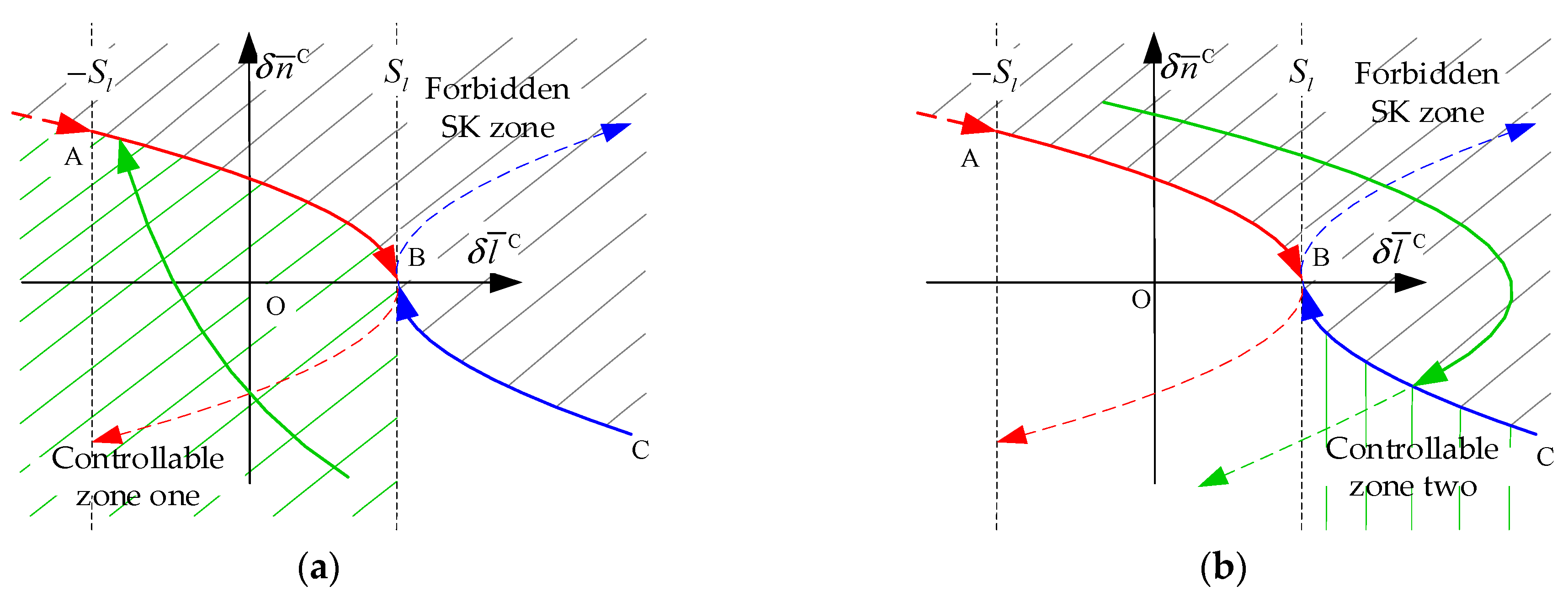
- (1)
- As shown in Figure 6a, when the initial mean longitude difference and the mean longitude drift rate is located in the controllable zone one, the same as the mean longitude based on a single-synovial surface, under the action of the tangential velocity increment, the sign of the mean longitude drift rate will change, and intersects with the synovial surface AB, and finally converges along the synovial surface AB near point B, forming a stable mean longitude keeping.
- (2)
- As shown in Figure 6b, when the initial mean longitude difference and the mean longitude drift rate is located in the controllable zone two, under the action of the tangential velocity increment, the mean longitude drift rate will change its sign and approach the synovial surface CB. If the synovial surface CB can be tracked in the controllable zone two, it will converge to the vicinity of point B along the synovial surface CB, forming a stable longitude keeping. If the synovial surface CB cannot be tracked in the controllable zone two, the control strategy switches to the controllable zone one, and finally converges along the synovial surface AB to the vicinity of point B, forming a stable longitude keeping.
- (3)
- As shown in Figure 6b, when the initial mean longitude difference and the mean longitude drift rate is located in the forbidden SK zone and is far away from the synovial surface AB and CB, under the action of the earth’s non-spherical gravitational force, the curve will move along the green parabola to the “controllable zone two”, which becomes the situation (2), and then becomes the situation (1), and finally realizes the stable mean longitude keeping. In addition, when the initial mean longitude difference and the mean longitude drift rate is located in the forbidden SK zone and is close to the synovial surface AB, it may be due to the surface modeling error of the synovial film, the curve will intersect with the synovial surface AB, and it will directly become the situation (1), and finally converge along the synovial surface AB to the vicinity of point B, forming a stable mean longitude keeping.
3.4. Adaptive Analysis of Control Strategy
4. Simulation and Analysis
4.1. Mean Longitude Keeping with Single-Synovial Surface
4.1.1. Example One
4.1.2. Example Two
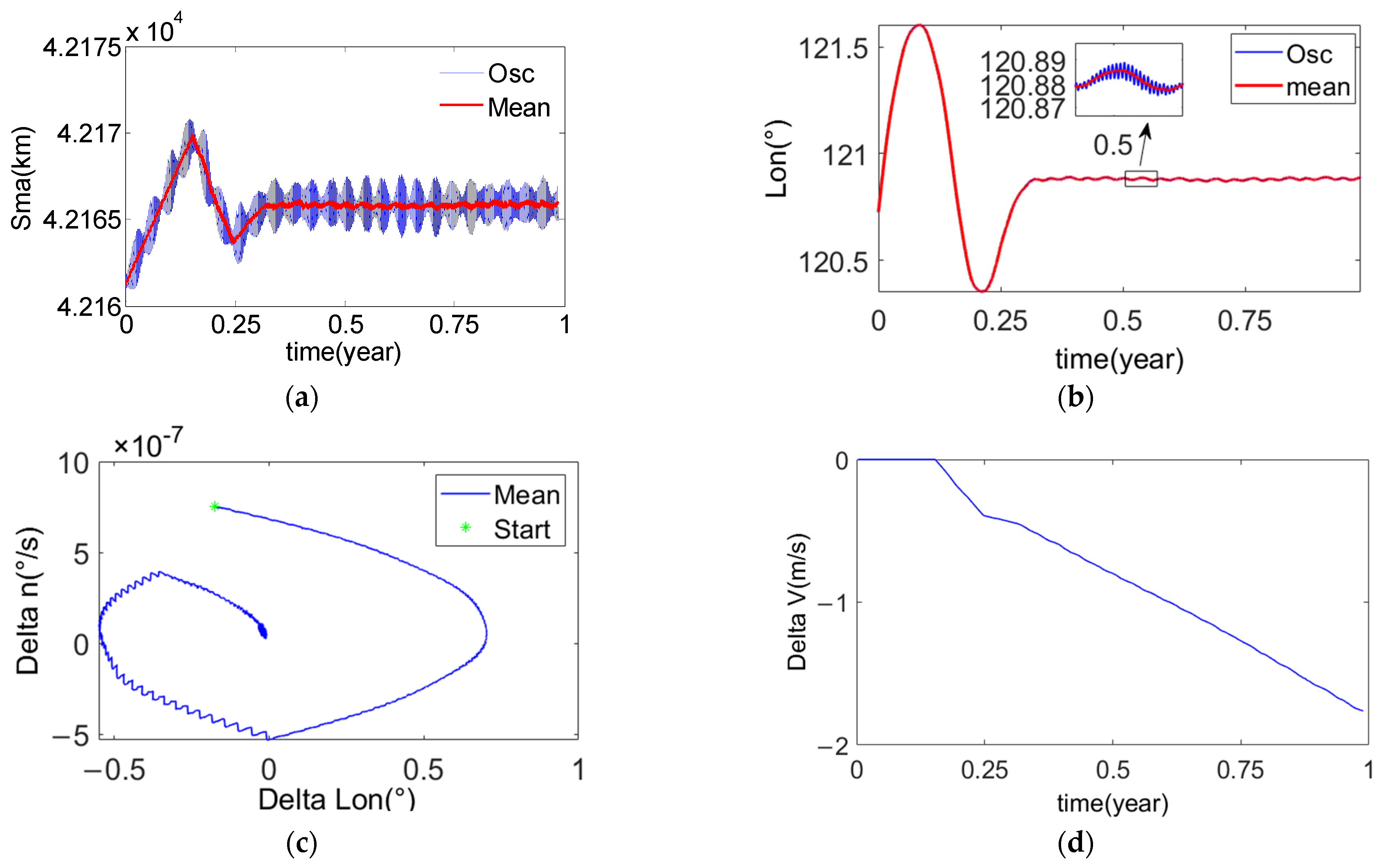
4.1.3. Example Three
4.1.4. Example Four
4.2. Mean Longitude Keeping with Dual Synovial Surface
4.2.1. Example One
4.2.2. Example Two
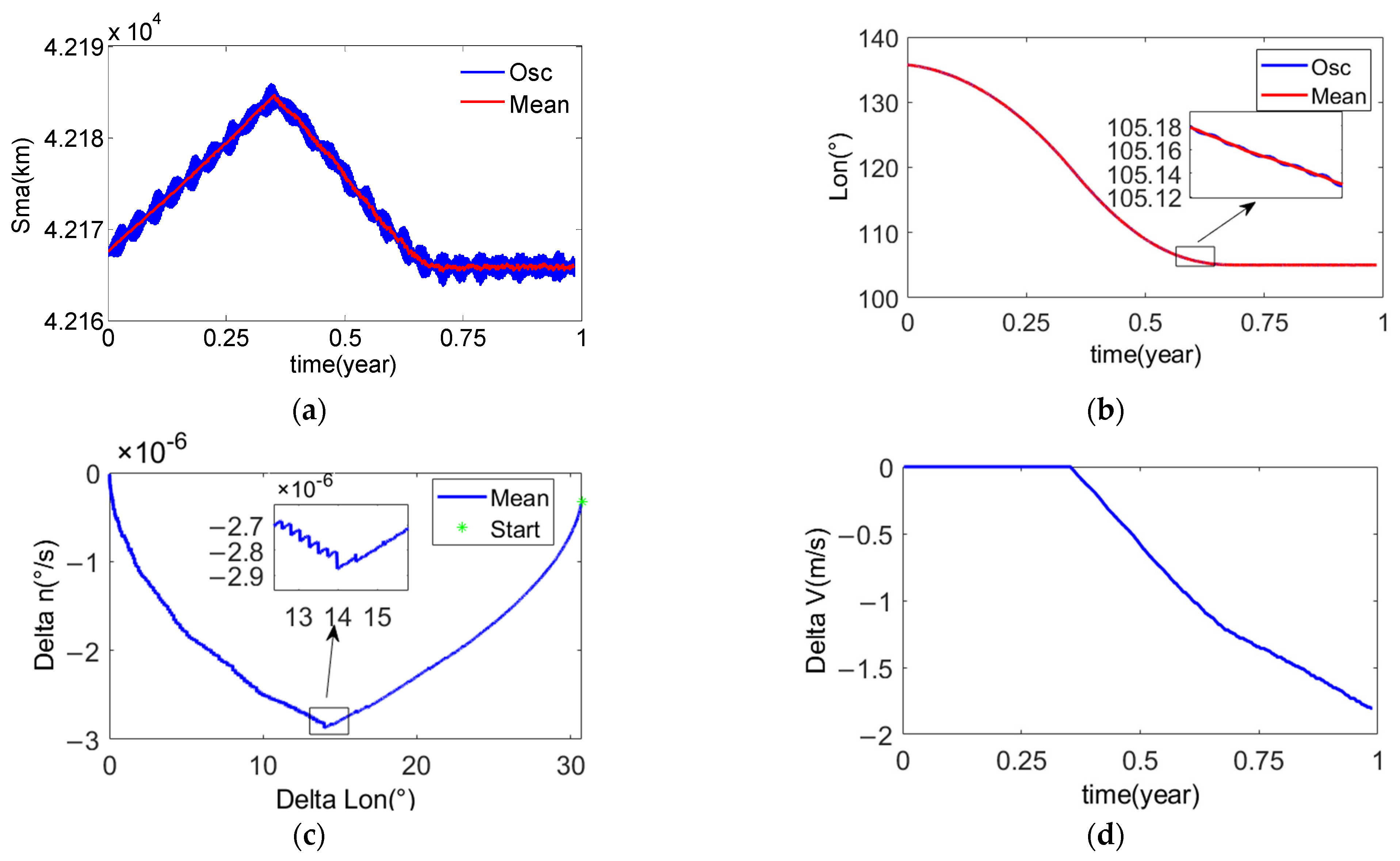
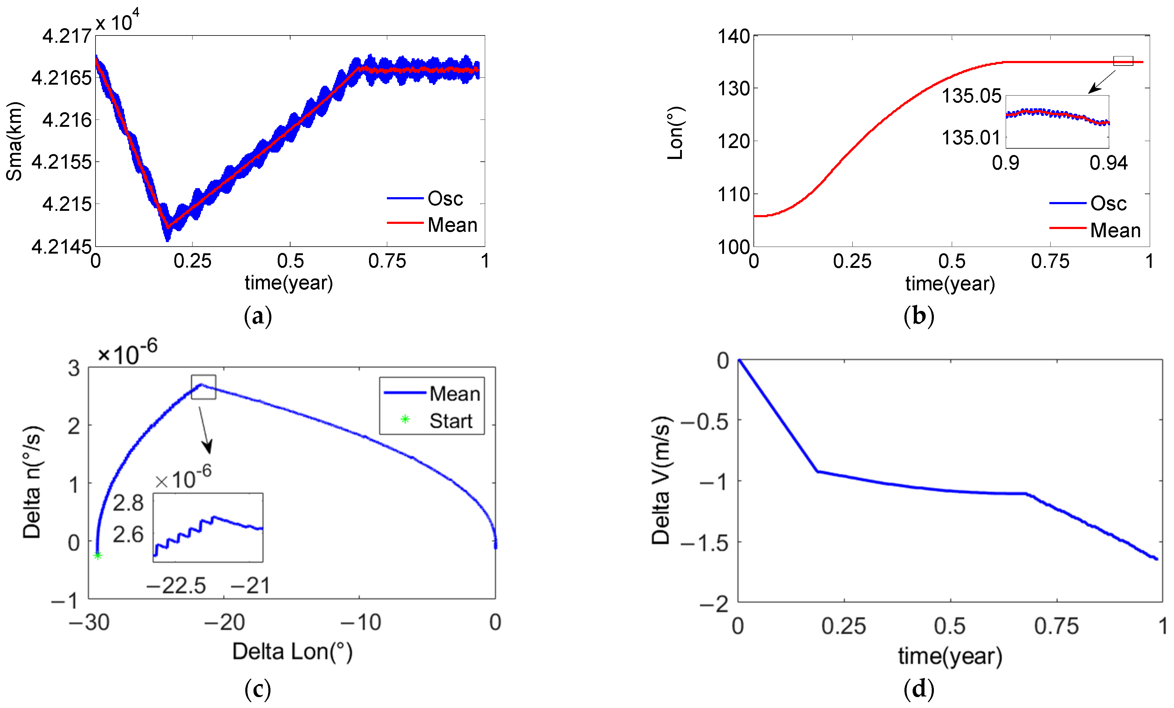
4.2.3. Example Three
5. Conclusions
Author Contributions
Funding
Data Availability Statement
Conflicts of Interest
References
- Chao, C.C. Applied Orbit Perturbation and Maintenance; The Aerospace Press: El Segundo, CA, USA, 2005. [Google Scholar]
- Wang, Z.C.; Xing, G.H.; Zhang, H.W. Handbook of Geostationary Orbits; National Defense Industry Press: Beijing, China, 1999. [Google Scholar]
- Ye, L.; Liu, C.; Zhu, W.; Yin, H.; Liu, F.; Baoyin, H. North/south Station Keeping of the GEO Satellites in Asymmetric Configuration by Electric Propulsion with Manipulator. Mathematics 2022, 10, 2340. [Google Scholar] [CrossRef]
- Possner, M.P.; Almendra, M.; Garcia, G. A New Flight Dynamics Solution for Operations of the Boeing 702 Satellite. In Proceedings of the AIAA Space 2008 Conference & Exposition, San Diego, CA, USA, 9–11 September 2008. [Google Scholar]
- Feuerborn, S.A.; Neary, D.A.; Perkins, J.M. Finding a way: Boeing’s All Elecric Propulsion Satellite. In Proceedings of the 49th AIAA/ASME/SAE/ASEE Joint Propulsion Conference, San Jose, CA, USA, 14–17 July 2013. [Google Scholar]
- Weiss, A.; Cairano, D. Station Keeping and Momentum Management of Low-thrust Satellites Using MPC. Aerosp. Sci. Technol. 2018, 76, 229–241. [Google Scholar] [CrossRef]
- Lin, S.Y.; Li, M.; Yang, Z. Position maintenance and momentum wheel unloading control of electric propulsion satellites based on model prediction and orbit recursion. In Proceedings of the 4th Annual Conference on High Resolution Earth Observation, Wuhan, China, 17–18 September 2017. [Google Scholar]
- Caverly, R.; Cairano, D.; Weiss, A. Split-Horizon MPC for Coupled Station Keeping, Attitude Control, and Momentum Management of GEO Satellites using Electric Propulsion. In Proceedings of the 2018 Annual American Control Conference (ACC), Milwaukee, WI, USA, 27–29 June 2018. [Google Scholar]
- Weiss, A.; Kalabic, U.; Cairano, S. Model Predictive Control for Simultaneous Station keeping and Momentum Management of Low-thrust Satellites. In Proceedings of the 2015 American Control Conference (ACC), Chicago, IL, USA, 1–3 July 2015. [Google Scholar]
- Walsh, A.; Cairano, D.; Weiss, A. MPC for coupled station keeping, attitude control, and momentum management of low-thrust geostationary satellites. In Proceedings of the 2016 Annual American Control Conference (ACC), Boston, MA, USA, 6–8 July 2016. [Google Scholar]
- Frederik, J.; Bruijn, D. Geostationary Satellite Station-Keeping Using Convex Optimization. J. Guid. Control Dyn. 2015, 39, 605–616. [Google Scholar]
- Gazzino, C.; Arzelier, D.; Cerri, L.; Losa, D.; Louembet, C.; Pittet, C. A Three-step Decomposition Method for Solving the Minimum-fuel Geostationary Station Keeping of Satellites Equipped with Electric Propulsion. Acta Astronatica 2019, 158, 12–22. [Google Scholar] [CrossRef] [Green Version]
- Gazzino, C.; Arzelier, D.; Losa, D.; Louembet, C.; Pittet, C.; Cerri, L. Optimal Control for Minimum-fuel Geostationary Station Keeping of Satellites Equipped with Electric Propulsion. IFAC Pap. Online 2016, 49, 379–384. [Google Scholar] [CrossRef]
- Gazzino, C.; Louembet, C.; Arzelier, D.; Jozefowiez, N.; Losa, D.; Cerri, C.P. Interger Programming for Optimal Control of Geostationary Station Keeping of Low-thrust Satellites. In Proceedings of the 20th IFAC World Congress 2017, Toulouse, France, 9–14 July 2017. [Google Scholar]
- Gazzino, C.; Arzelier, D.; Cerri, L.; Pittet, C.; Losa, D. Long-Term Electric-Propulsion Geostationary Station-Keeping via Integer Programming. J. Guid. Control Dyn. 2019, 42, 976–991. [Google Scholar] [CrossRef]
- Sukhanov, A.A.; Prado, A.F. On one Approach to the Optimization of Low-thrust Station Keeping Manoeuvres. Adv. Space Res. 2012, 50, 1478–1488. [Google Scholar] [CrossRef]
- Roth, M. Strategies for Geostationary Spacecraft Orbit SK Using Electrical Propulsion Only. Ph.D. Thesis, Czech Technical University, Prague, Czech Republic, 2020. [Google Scholar]
- Ogawa, N.; Terui, F.; Mimasu, Y.; Yoshikawa, K.; Ono, G.; Yasuda, S.; Matsushima, K.; Masuda, T.; Hihara, H.; Sano, J.; et al. Image-based autonomous navigation of Hayabusa2 using artificial landmarks: The design and brief in-flight results of the first landing on asteroid Ryugu. Astrodyn 2020, 4, 89–103. [Google Scholar] [CrossRef]
- Wang, Y.; Xu, S. Non-equatorial equilibrium points around an asteroid with gravitational orbit-attitude coupling perturbation. Astrodyn 2020, 4, 1–16. [Google Scholar] [CrossRef]
- Zhang, T.J.; Wolz, D.; Shen, H.X.; Luo, Y.-Z. Spanning tree trajectory optimization in the galaxy space. Astrodyn 2021, 5, 1–16. [Google Scholar] [CrossRef]


| Model Type | Description |
|---|---|
| Gravity Model | Earth’s Gravitational Field: EGM2008 100 × 100 Solid Tide: IERS 96 Polar Tide: IERS 96 Sea Tide: CSR 4.0 Third Body Gravity: DE405 |
| Non–conservative Force Model | Sunlight Pressure: cannonball Model Atmospheric Drag: Jacchia 71 Model |
| Initial Conditions | Illustrate | Process | ||
|---|---|---|---|---|
| Example one | Chief satellite is in the controllable zone | 1 | Lower orbital height → drift naturally → capture | |
| Example two | Chief satellite is in the controllable zone | 0.8 | Lower orbital height → drift naturally → capture | |
| Example three | Chief satellite is in the forbidden SK zone two | 0.8 | Drift naturally → capture | |
| Example four | Chief satellite is in the forbidden SK zone one | 0.8 | Drift naturally → capture |
| Name | Value |
|---|---|
| Orbital semi-major axis of the chief satellite (km) | 42,167.300 |
| Mean longitude of the target satellite | 123.500 |
| Initial mean longitude of the chief satellite | 120.725 |
| Name | Value |
|---|---|
| Orbital semi-major axis of the chief satellite (km) | 42,161.300 |
| Mean longitude of the target satellite | 120.900 |
| Initial mean longitude of the chief satellite | 120.725 |
| Name | Value |
|---|---|
| Orbital semi-major axis of the chief satellite (km) | 42,161.300 |
| Mean longitude of the target satellite | 110.500 |
| Initial mean longitude of the chief satellite | 120.725 |
| Initial Conditions | Illustrate | Process | ||
|---|---|---|---|---|
| Example one | Chief satellite is in the forbidden SK zone | 1 | Drift naturally → lower orbital height → capture | |
| Example two | Chief satellite is in the forbidden SK zone | 0.8 | Drift naturally → lower orbital height →capture | |
| Example three | Chief satellite is in the controllable zone | 0.8 | Lower orbital height → drift naturally → capture |
| Name | Value |
|---|---|
| Orbital semi-major axis of the chief satellite (km) | 42,167.300 |
| Mean longitude of the target satellite | 105 |
| Initial mean longitude of the chief satellite | 135.725 |
| Name | Value |
|---|---|
| Orbital semi-major axis of the chief satellite (km) | 42,161.300 |
| Mean longitude of the target satellite | 135 |
| Initial mean longitude of the chief satellite | 105.725 |
Disclaimer/Publisher’s Note: The statements, opinions and data contained in all publications are solely those of the individual author(s) and contributor(s) and not of MDPI and/or the editor(s). MDPI and/or the editor(s) disclaim responsibility for any injury to people or property resulting from any ideas, methods, instructions or products referred to in the content. |
© 2023 by the authors. Licensee MDPI, Basel, Switzerland. This article is an open access article distributed under the terms and conditions of the Creative Commons Attribution (CC BY) license (https://creativecommons.org/licenses/by/4.0/).
Share and Cite
Liu, F.; Ye, L.; Liu, C.; Wang, J.; Yin, H. Micro-Thrust, Low-Fuel Consumption, and High-Precision East/West Station Keeping Control for GEO Satellites Based on Synovial Variable Structure Control. Mathematics 2023, 11, 705. https://doi.org/10.3390/math11030705
Liu F, Ye L, Liu C, Wang J, Yin H. Micro-Thrust, Low-Fuel Consumption, and High-Precision East/West Station Keeping Control for GEO Satellites Based on Synovial Variable Structure Control. Mathematics. 2023; 11(3):705. https://doi.org/10.3390/math11030705
Chicago/Turabian StyleLiu, Fucheng, Lijun Ye, Chunyang Liu, Jingji Wang, and Haining Yin. 2023. "Micro-Thrust, Low-Fuel Consumption, and High-Precision East/West Station Keeping Control for GEO Satellites Based on Synovial Variable Structure Control" Mathematics 11, no. 3: 705. https://doi.org/10.3390/math11030705