Article

Numerical Investigation of Internal Flow Properties around Horizontal Layered Trees by Using the Reynolds Stress Model

1
Graduate School of Science and Engineering, Saitama University, Saitama 338-8570, Japan
2
Department of Civil Engineering, COMSATS University, Abbottabad Campus, Islamabad 22060, Pakistan
3
International Institute for Resilient Society, Saitama University, Saitama 338-8570, Japan
*
Author to whom correspondence should be addressed.
Mathematics 2023, 11(3), 712; https://doi.org/10.3390/math11030712
Submission received: 28 December 2022 / Revised: 26 January 2023 / Accepted: 29 January 2023 / Published: 31 January 2023

Abstract

:
The aim of this article is to numerically explore the effects of a horizontal double layer of trees (HDLT) across the whole width of the channel on the flow structures under a steady flow rate and subcritical conditions. The numerical domain was established in ANSYS Workbench, and post-processing (i.e., meshing + boundary conditions) along with simulation was carried out by utilizing the computational fluid dynamics tool FLUENT. The three-dimensional (3D) Reynolds stress model and Reynolds-averaged Navier–Stokes equations were used to analyze the flow properties. The numerical model was first validated and then used for simulation purposes. Two varying configurations of HDLT were selected, represented as Arrangement 1 (tall emerged trees (Tt) + short submerged trees (St)) and Arrangement 2 (short submerged trees (St) + tall emerged trees (Tt)), along with different flow heights. The model accurately captured the simulated results, as evidenced by the vertical distributions of the velocity profiles and Reynolds stresses at specific locations. The strong inflection in velocity and Reynolds stress profiles was observed at the interface of St, contributing to turbulence and giving rise to vertical transportation of momentum between flow layers. While these profiles were almost constant from the beds to the tops of trees at those locations lying in taller trees (Tt), there was an approximate 31–65% increase in streamwise velocities at locations 1–6 in cases 1–2, along with a 54–77% increase at locations 7–10 in cases 3–4, in the unvegetated zone (Z > 0.035 m) compared to the vegetated zone (Z < 0.035 m). The magnitude of turbulence kinetic energy and the eddy dissipation rate were significantly larger inside the short submerged and tall emerged trees as compared to the unvegetated region, i.e., upstream and downstream regions. Similarly, the production of turbulence kinetic energy was approximately 50% and 70% greater inside the tree region (Z < 0.035 m) as compared to above the shorter trees during cases 1–2 and 3–4, respectively.

1. Introduction

Tsunamis are catastrophic because they can destroy manmade structures and natural landscapes, and they can even take human lives [1]. Two massive tsunamis (2004, Indian Ocean; 2011, Great East Japan) occurred at the beginning of the 21st century, causing devastating havoc [2,3]. Tsunami defenses became a necessity after these massive tragedies. Several artificial (hydraulic infrastructure) and natural (coastline vegetation) approaches have been suggested for tsunami prevention [4]. Artificial structure development may be out of reach for certain developing nations because of the high initial capital outlay that is usually required [5]. Therefore, studies have concentrated on the importance of natural structures such as coastline vegetation, since they are regarded as an effective source of tsunami prevention and promote an ecologically friendly environment [6,7,8,9]. Data collected in Sri Lanka during the 2004 Indian Ocean Tsunami confirmed that vegetation with a double layer consisting of short (P. odoratissimus) and tall trees (C. equisetifolia) provided efficient protection against the tsunami. P. odoratissimus is efficient in mitigating tsunamis’ impact when the tsunami’s height is less than 5 m [10], due to the plant’s extensive aerial roots. As a result, several experimental investigations have focused on elucidating the efficacy of a VDLV (short trees among tall trees) [11,12,13]. However, growing dense shorter trees among the large trees is difficult, since the large trees need enough space to grow properly. Thus, to address the problem of insufficient space for the effective growth of tall emergent trees, this research utilizes the combination of a horizontal double layer of dense short trees as the first row, with the sparse tall trees as the second row (i.e., HDLT), and then changes the order of these two tree combinations one by one. Additionally, owing to equipment restrictions inside the vegetation region, capturing the flow characteristics among the vegetation cylinders during an experimental trial is quite difficult. To clarify the internal flow characteristics throughout this work, numerical simulation was carried out.
However, multiple numerical simulations on vegetation [14,15,16,17,18,19,20,21] have been performed to better comprehend their fundamental flow features. The turbulence flow characteristics were explored in a vegetated open channel by utilizing a large-eddy simulation (LES) model [22,23]. To analyze the flow and transport of sediments with a tree in an open channel, Wu et al. [24] used a depth-averaged two-dimensional (2D) k-ε model. Amina and Tanaka [25] utilized the volume-of-fluid (VOF) model to explore the free surface variations around a finite patch of emergent trees. In addition, the flow structure behavior around discontinuous and submerged trees was explored by Zhao and Huai [26] by utilizing LES. Furthermore, to dissipate the energy of tsunami flows, numerous studies have been conducted by planting trees as a barrier to stop the tsunami flow [27,28,29,30,31].
An earlier numerical analysis by Samarakoon et al. [32] used short trees as a front layer to lessen the impact of open gaps (such roads or rivers) among the pre-existing tall trees. However, no research on the utilization of this type of horizontal double layer of trees (HDLT) has been performed. As a result, it is important to examine the precise flow structure, including velocity and turbulent flow, utilizing an HDLT. Thus, the purpose of this study was to precisely investigate the internal flow characteristics of HDLT in terms of a detailed three-dimensional (3D) velocity structure and other flow parameters. Moreover, the use of electromagnetic flow meters (EFMs) or particle image velocity meter (PIV) for velocity measurement and shear stress meters (SSMs) for measuring bed shear stresses is limited within the trees’ area, making it difficult to capture the flow structure within the trees’ cylinders in an experimental study. The current numerical research was successful in avoiding this problem, which was one of its main advantages. To achieve this aim, a numerical study was conducted with two tree layouts: one with a short submerged patch as a first layer and a tall emergent patch as a back layer, and the other with a tall emergent patch as a first layer and a short submerged patch as a back layer. The detailed comparison between these two patches is presented in the form of 3D mean flow properties and turbulence characteristics.

2. Governing Mathematical Equations of Reynolds-Averaged Navier–Stokes (RANS) Equations for the RSM Model

The continuity and the Reynolds-averaged Navier–Stokes (RANS) equations were used to represent a steady, incompressible flow ( ρ = CONSTANT ) for the present numerical model.
In the present study, the considered flow was steady, and the density was constant; therefore, D p t = 0 . The continuity and (RANS) equations can be expressed as follows:
u i x i = 0
For incompressible flow, the Navier–Stokes equation is stated as follows:
d u i d t + u j d u i d x j = 1 ϱ p X i + g i + υ 2 u i
For the above equation, the variables stand for the following:
u = Velocity of fluid;
t = Time;
p = Fluid pressure;
υ = Kinematic viscosity;
2 = Laplacian operator.
The equation below represents the modified relation for the transport of Reynolds stresses:
R i j t + C i j = P i j + D i j ε i j + Π i j + Ω i j
where R i j denotes the rate of change of the Reynolds stresses, C i j is the transport of convection, P i j represents the production rate of the Reynolds stresses, D i j is the transport of stresses by diffusion rate, ε i j is the rate of dissipation for stresses, Π i j is a function of the stresses’ transport, and Ω i j is the transport of stresses due to rotation.
In order to accomplish the boundary conditions, the equation for Reynolds stresses known as the turbulence kinetic energy (TKE) equation was used. This equation can be expressed in a generic form as follows:
t ( ρ k ) + x i ( ρ k u i ) = x j [ ( μ + μ t σ k ) k x j ] + 1 2 [ P i i + G i i ] ρ ε ( 1 + + 2 M t 2 ) + S k
The variables are expressed as follows:
k = Kinetic energy tensor;
μ t = Turbulent viscosity;
σ k = 0.82;
ε = Rate of dissipation;
S k = Source term.
The kinetic energy tensor term is stated as follows:
k = 1 2 u i u i ¯
The rate of dissipation ( ε ) can be expressed by the following equation:
t ( ρ ε ) + x i ( ρ ε u i ) = x j [ ( μ + μ t σ ε ) ε x j ] C ε 1 1 2 [ P i i + C ε 3 G i i ] ε k C ε 2 ρ ε 2 k S ε
where the values of the variables are represented as follows: σ ε = 1.0 , C ε 1 = 1.44, C ε 2 = 1.93 , and C ε 3 represents a function of the direction of flow with respect to the gravitational vector and can be expressed and estimated by using the following equation:
C ε 3 = tanh | v u |
where v is the velocity flow component and u denotes a component of velocity that is perpendicular to the gravitational vector.
μ t = ρ C μ K 2 ε
The value of C μ is 0.09.

3. Materials and Methods

3.1. Conditions for Validation of the Numerical Model

3.1.1. Experimental Setup

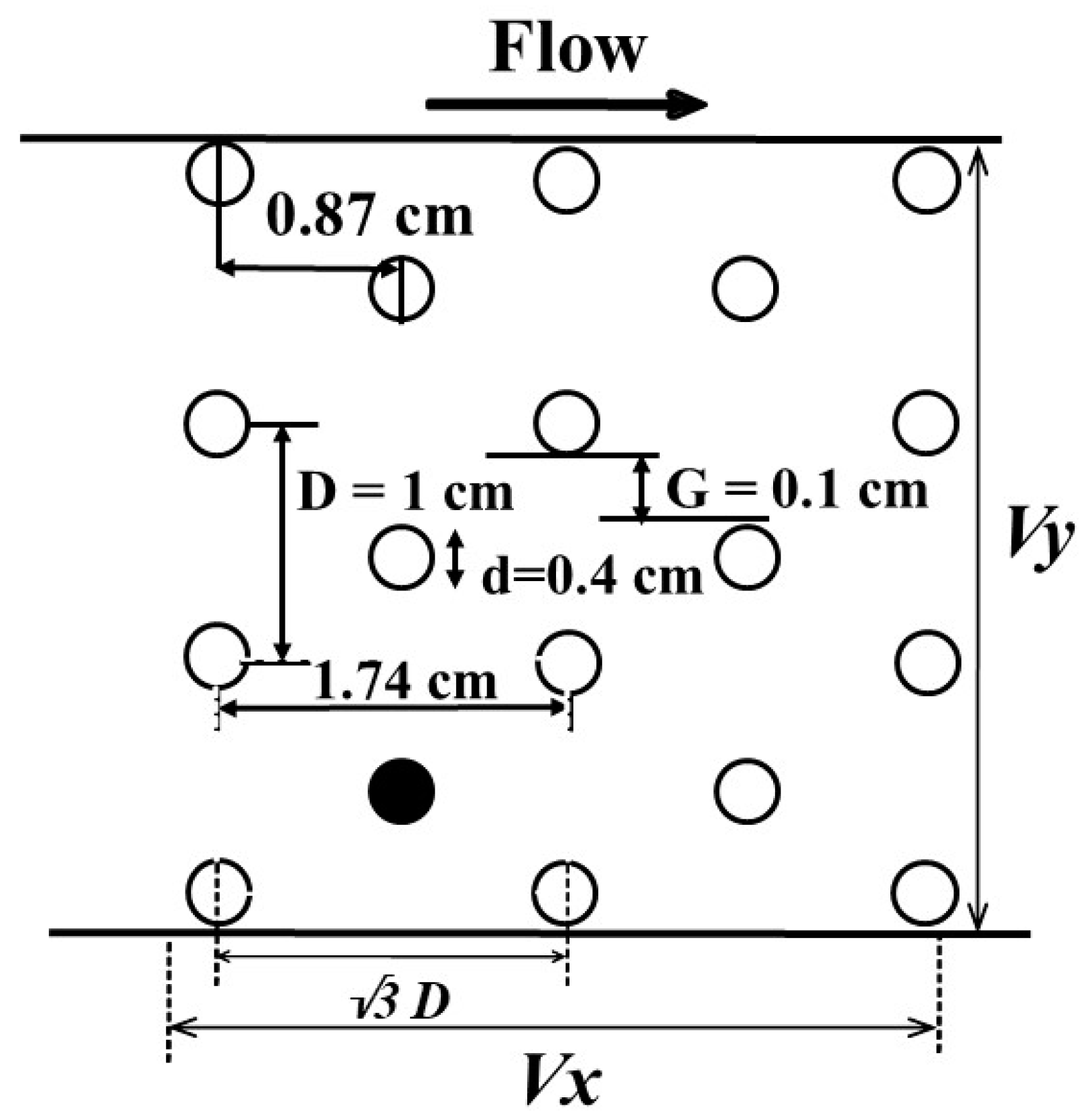
The numerical model was tested and verified to ensure its accuracy and applicability through validation. As a result, the experimental data of [33] were employed as the basis for validation. The velocity profiles were extracted while considering the vertically double-layered vegetation. The vegetation consisted of short and tall trees, where short trees were installed amongst the tall trees. The diameter of both types of trees was considered as 0.635 cm, while the heights of the tall and short tress were 15.2 cm and 7.5 cm, respectively. The dimensionless spacing between short (Sst) and tall (Sts) trees was set to 5 and 10, respectively (where Sst defines the spacing between short tress and Sts denotes the spacing between tall trees). The vegetation layer was configured in a staggered arrangement. The layout of the vegetation is presented in Figure 1.

3.1.2. Numerical Model Setup

In order to prevent a massive mesh structure and save computational cost, the channel length was shortened in order to simplify the geometry. The domain was modelled with a length of 75 cm and a width of 30 cm, in which double-layered vegetation was incorporated. The calculated flow depth was 12 cm; therefore, the domain depth was adopted as the same. Accordingly, the domain’s measurements were 75 cm long, 30 cm broad, and 12 cm deep. The trees were modelled as solid cylinders of the same diameter to allow for flow interaction with the structures of the vegetation. The multizone meshing was adopted for this simulation. The details of the preprocessing (i.e., geometry creation and meshing) and post-processing (i.e., setup and boundary conditions) are discussed in Section 3.2.4. Approximately 1.55 million grid points were generated from the meshing of a domain with dimensions of 350 nodes in the stream direction, 150 nodes in the transverse direction, and 50 nodes in the depth direction. Moreover, quality outcomes were achieved by a trial for a mesh independence test. Initially, mesh grids of 140 × 50 × 25 (0.15 million, coarse), 350 × 150 × 50 (1.55 million, medium), and 370 × 170 × 35 (2.00 million, fine) were tested. The primary velocity differences between the coarse and medium meshes were approximately 4%, whereas those between the medium and fine meshes averaged around 1%, which was appropriate. Thus, the 1.55-million-grid mesh was chosen for further analysis.
To maintain continuity (i.e., translational periodicity) throughout the channel domain, a periodic boundary condition was imposed at the channel’s inlet and outlet. For the top free surface, a symmetrical boundary condition was implemented. For the side, bed, and cylinder walls, a no-slip BC was employed. The inlet of the channel was subjected to a flow rate of 11.5 L/s, with mean averaged velocities of 0.35 m/s for high flow depth and 0.65 m/s for low flow depth, and the corresponding cylinder Reynolds numbers were roughly 1950 and 4025, respectively.

3.1.3. Validation of the Numerical Model

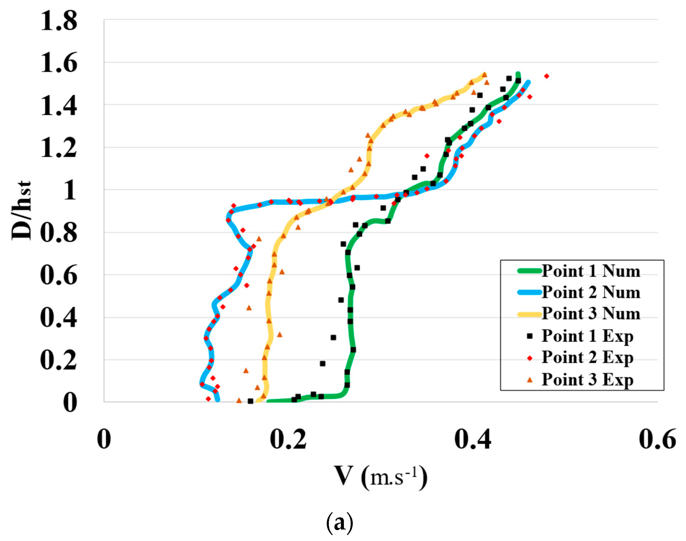
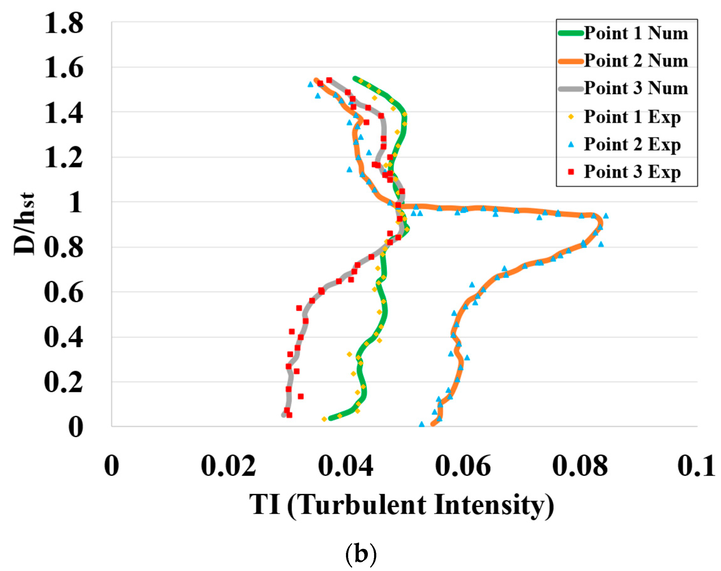
The computed velocity and turbulence intensity profiles were computed and compared with the experimental results of the abovementioned previous research. The velocity (Figure 2a) and turbulence intensity (Figure 2b) were depicted on the X-axis, while the flow depth—which was normalized with the short trees’ height—was on the Y-axis. Three positions were selected, where the velocity and turbulence intensity were measured along the depth of flow. The calculated outcomes matched the experimental outcomes quite well and showed a high degree of similarity, while a small difference between the computed and experimental results could be seen near the free surface level 1.4     D h s t 1.5 , because in this simulation the top free surface was assigned a symmetrical boundary condition, which means that the upper boundary was treated as a flat surface. Second, the difference in pressure created by the water level difference inside the vegetation in the actual flow enhanced the velocity at the free surface level [34,35,36].

3.2. Conditions for the Present Numerical Model

3.2.1. Flow Conditions for the Numerical Model

During the Great East Japan Tsunami (GEJT) of 2011, subcritical flows occurred at multiple sites in an inland forest in Miyagi Prefecture, Japan. The Froude numbers at these locations ranged from 0.7 to 1, and the estimated inundation depth was between 7.3 and 8.3 m [3]. Furthermore, the Fr values in the region of Banda Aceh were calculated at 0.64–1.04 [37]. To replicate a real-scale flow while keeping the Froude number constant, a model size/scale of 1/100 and two flow conditions were employed. Thus, without taking into account a model of trees in the rectangular channel, the values of water depth and velocity were used to establish the initial Froude number ( F r = u g d , where u is the velocity of the water, g denotes a gravitational constant, and d is the depth of the water). This numerical work established the subcritical inland flow conditions at water depths of 6 and 8 cm, yielding initial Froude numbers of 0.65 and 0.68, respectively (without a trees model).

3.2.2. Model Conditions for Trees

Existing trees in Sendai Plain, Japan, had densities, trunk heights, and diameters of 0.2 trees/m2, 15 m, and 0.4 m, respectively. During the 2004 Indian Ocean Tsunami (IOT), C. equisetifolia trees in Sri Lanka with trunk diameters greater than 0.3 m were positioned in the front line of trees, and Tanaka et al. [38] showed that they were undamaged and capable of capturing human-made debris and broken tree limbs. In addition, these trees with large trunk diameters were identified as having sparse tree density (i.e., greater spacing between individual trees). Another tree species, P. odoratissimus, has been found to be useful because of its dense organization and complicated aerial roots [39], which increase the drag coefficient [40] and, hence, provide extra protection against flood flows. It has been shown that these trees are most effective when the flow height is less than 5 m, and people living in the areas immediately behind these trees suffered minimal damage. Furthermore, Zheng et al. [41] revealed that in order to replicate the P. odoratissimus trees for modeling, they can be scaled down to rigid circular cylinders by considering the trunk diameter at its breast height. Therefore, in the current computational simulation, horizontal double layer of trees (HDLT) models with two different arrangements were considered. The first arrangement comprised a first half patch of short trees (P. odoratissimus) and a remaining half patch of tall trees (C. equisetifolia), whereas the order of the considered trees was then changed in the second arrangement. In order to better understand the internal flow behavior, this research ignored the assumption that trees may be broken as part of an actual flow behavior via the HDLT model. The diameter of both patches of trees was calculated based on the non-breaking tree trunk diameter criteria (d > 40 cm). As a result, with a model scale of 1/100, a diameter (d) of 0.004 m was chosen in the numerical modelling to represent a tree cylinder. The tall tree height ( h t ) was fixed at 18 cm to represent the trunk of the C. equisetifolia trees, while the short tree height ( h s ) was fixed at 3.5 cm to mimic the small height of P. odoratissimus trees.
The D/d value determines the density of the trees [10]. This D/d ratio shows whether the trees’ configuration is sparse, moderate, or dense. D represents the clear spacing between the located cylinders in a transverse flow, while d denotes the cylinder’s diameter. According to the previous literature regarding the calculation of trees’ density [10], the D/d values were chosen as 2.15 and 0.0425 for tall (emerged) and short (submerged) trees, respectively.

3.2.3. Selected Cases and Measurement Positions

The current domain was represented by a rectangular channel that was 2 m long and 0.3 m wide and had an HDLT that covered the whole breadth of the domain in two different arrangements (Figure 3 and Figure 4). In the first arrangement, a short submerged patch ( P S ) provided the front layer and a tall emergent patch ( P t ) provided the rear layer, while in the second arrangement P t was located as the front layer and P S as the back layer (Figure 3). Overall, four cases were chosen based on the flow conditions and arrangement types. The hydraulic conditions and the trees’ conditions are presented in Table 1. To investigate and visualize the internal flow behavior through the HDLT, Section 1 (for visualizing the turbulent parameters, i.e., TKE and TDR) was considered, which was aligned along the centerline of the channel and trees. Overall, 10 locations were selected to understand the internal flow features, including vertical velocity profiles and the distribution of Reynolds stresses.

3.2.4. Preprocessing and Post-Processing

The ANSYS computational fluid dynamics tool was used to simulate the present numerical model. This research utilized a two-stage numerical setup consisting of preprocessing and post-processing. During preprocessing, WORKBENCH—a design modeler tool—was utilized to model the geometry. In the WORKBENCH tool, a rectangular channel of 200 cm long and 30 cm broad was created along with the tree cylinders (placed in a staggered arrangement) that covered the entire width of the channel. Figure 3 depicts the cylinder placement and spacing in the trees model. Once the geometry was created, it was then transferred to a mesh tool for meshing. Effective meshing, which is defined as the splitting of the geometry into components such as cells and elements, is a crucial step and is necessary in producing high-quality results. The simulation’s accuracy, convergence, and runtime are all affected by the mesh size and density. Fine meshing requires more memory and time, while inaccurate meshing leads to incorrect results. Therefore, we first tried out several different meshing techniques in a vegetated open channel (e.g., sweep meshing, tetrahedral primitive with numerous deformable components resulted in higher skewness values and, in some cases, negative volumes); however, multizone meshing with hexahedral components yielded convergence with a reasonable computation time. When defining a boundary, the tetrahedral meshing’s exclusive use of tetra cells prevented a balanced distribution of cells. A low-quality surface mesh surrounding the tree cylinders was also produced by this method. However, multizone meshing, which combines hexahedral or brick elements with tetra elements, typically yields more accurate results at lower element counts than tetra elements alone. Moreover, the mesh quality was assessed using the skewness and orthogonal quality criterion techniques. The degree of skewness indicates how far a face or cell deviates from the ideal (equiangular quad). The definition states that a value of 0 denotes “Excellent”, while a value of 1 indicates the worst possible quality of cells (i.e., degenerate). Skewness was evaluated in this study using the equilateral volume-based technique. As per this technique, a 3D mesh is of high quality if its skewness is less than 0.35. Here, the mesh quality of the geometry being used was 0.14, which is very high. Then, the names were assigned to the faces of the geometry. The front face was given the term water inlet, while the back side was given the name outlet. For the side faces, the downward faces and tree cylinders were named as solid walls. The top surface was assigned as a free surface or symmetry.
After meshing and assigning the names, the geometry was shifted to the post-processing process. The three-dimensional (3D) Reynolds stress model (RSM) was utilized for setting up the physics and for the turbulence closure model. It has been noted that the RSM provides the most accurate simulation of the non-isotropic structure of the flows for both the empty and vegetated open-channel flow problems. Furthermore, it has been observed that the RSM is preferable to the other models in predicting the mean flow and turbulence characteristics considering the open-channel flow with submerged vegetation inside the channel [36]. In this simulation, we took both submerged and emergent vegetation in an open channel; therefore, we used this model to obtain good outcomes. After that, boundary conditions were applied to the faces of the geometry that were previously assigned in the meshing process. The periodic boundary condition was implemented at the inlet/outlet to ensure the translational periodicity and uniform flow features. A symmetrical boundary condition was used for the top free surface. The domain’s cylinders, sides, and bed walls were all given to a no-slip wall condition. For the convergence criterion and residual smoothing, low under-relaxation factor values were selected. For solution initialization, the conventional initialization procedure was employed. The method, governing equations, and turbulence model are all described in the user guide [42].

4. Results and Discussion

4.1. Vertical Distribution of Velocities

4.1.1. Vertical Distribution of Longitudinal Velocity (u)

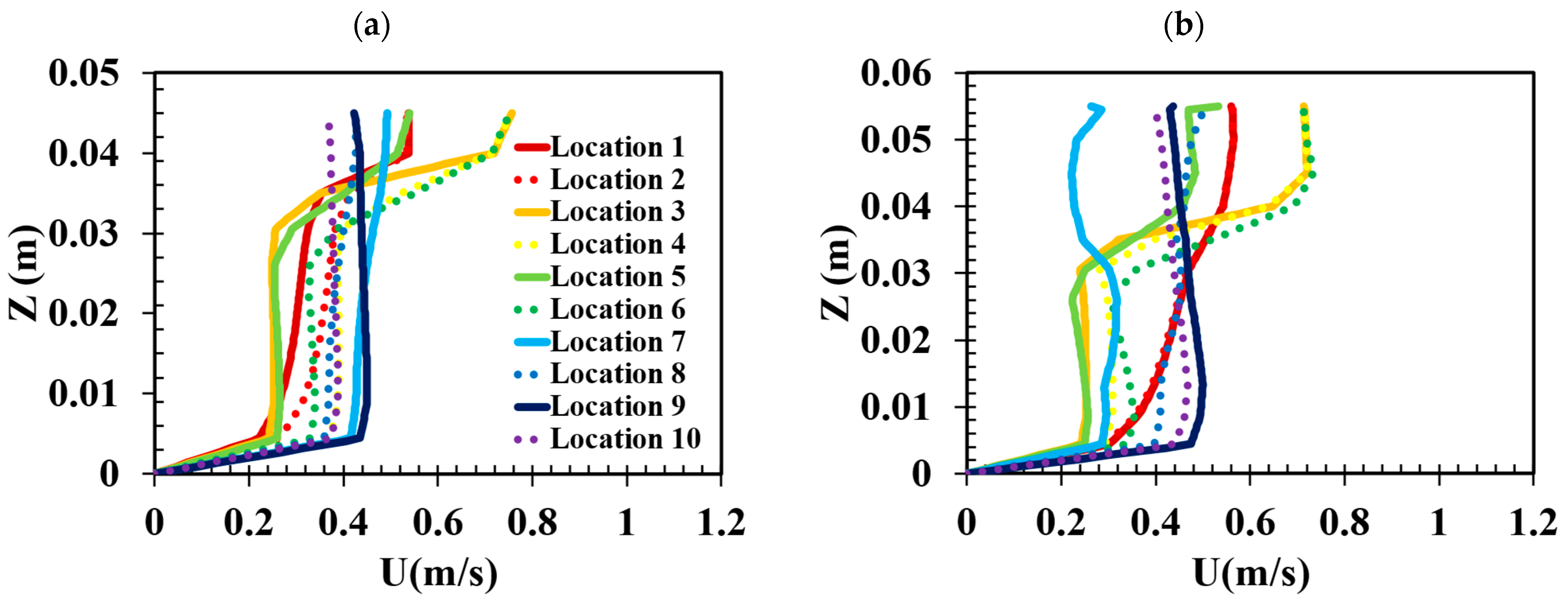
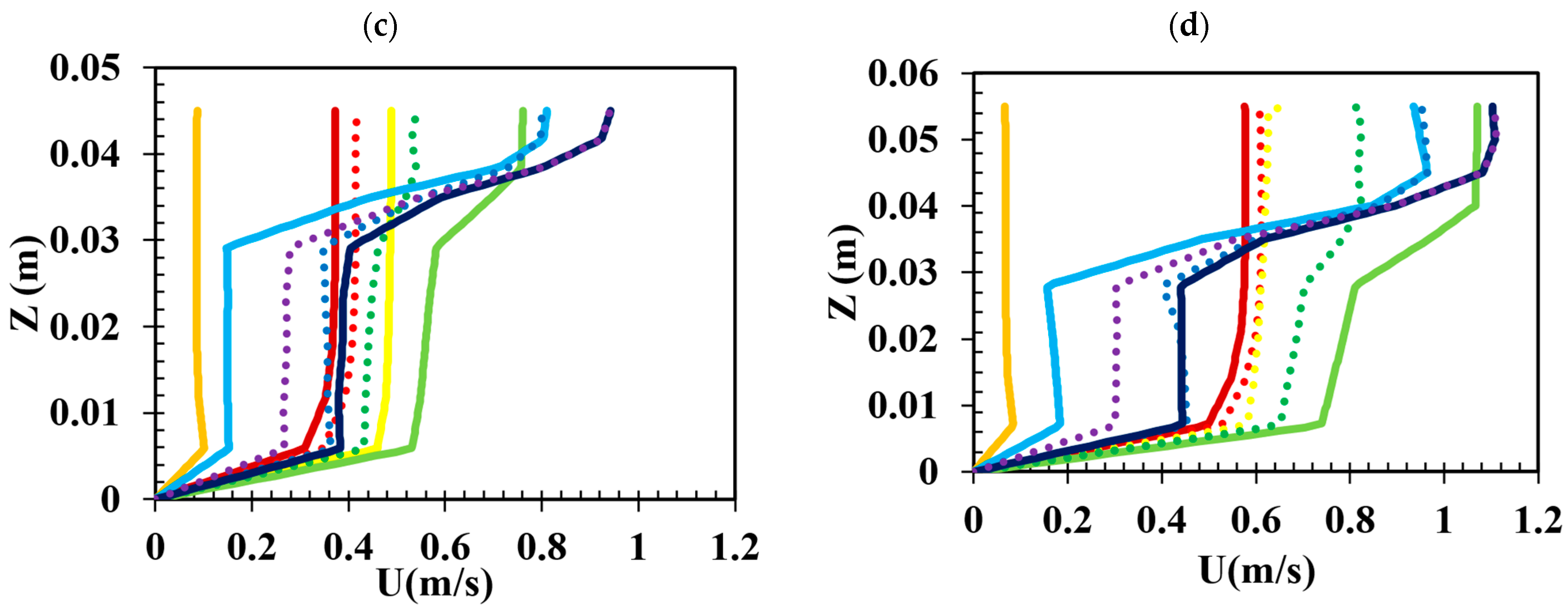
The calculated results for the vertical distribution of the longitudinal velocity component (u) at specific locations for each of the four cases are shown in Figure 5a–d. The X-axis represents the longitudinal component of velocity (u), while the Y-axis represents the vertical component of water depth (Z). From Figure 5, it is clear that three distinct portions of the plots—portions 1, 2, and 3—can be distinguished at all locations that are inside, directly upstream, or downstream of shorter submerged layers (i.e., locations 1–6 in cases 1–2 and locations 5–10 in cases 3–4.
Portion 1 of the plots is situated among the short trees adjacent to the bed. In all cases, at the aforementioned locations, the longitudinal component of velocity (u) in portion 1 has a minimal value near the bed and exhibits a linear gradient with an increasing pattern along with the depth of water. The resistance provided by the bed is the source of the minimal value of the longitudinal component of velocity close to the bed. Meanwhile, the second portion of the plots lies within the submerged/short trees (below the tops of the short trees (Z ≤ 0.035 m)), and the longitudinal velocity component (u) is almost constant along with the water depth towards the tops of the short trees. The third portion of the plot consists of an inflection point near the tops of the short trees (Z = 0.035 m), where the longitudinal velocity component is increased above the tops of the short trees because there is no hindrance or resistance by the shorter trees due to the momentum being exchanged between overlying flow and the tops of the short trees. This zone is known as the shear zone [43], and it has the highest intensity of vortices; similar behavior was reported by [21,44,45,46]. While the behavior of the velocity profile in cases 1–2 at locations 7–10 and in cases 3–4 at locations 1–4 (found in tall trees) is remarkably similar, these locations are in taller trees. The plots of these locations consist of two portions: during the first portion, the longitudinal velocity component is very small near the bed and increases towards the tops of the trees up to a certain flow depth. while in the second portion of the plot the velocity component is almost constant toward the tops of the tall trees because the tall trees continued to provide resistance to flow up to the tops of the trees. The magnitude of the longitudinal velocity component in all cases is comparatively greater at locations 2, 4, 6, 8, and 10 (located in the gap regions between cylinders) as compared to locations 1, 3, 5, 7, and 9 (located in line with the cylinders). Inside the short trees (i.e., Z < 0.035 m), 30–64% reductions in the velocities in cases 1–2 and 53–78% reductions in the velocities in cases 3–4 were observed as compared to above the submerged trees (i.e., Z > 0.035 m).

4.1.2. Vertical Distribution of Lateral Velocity (v)

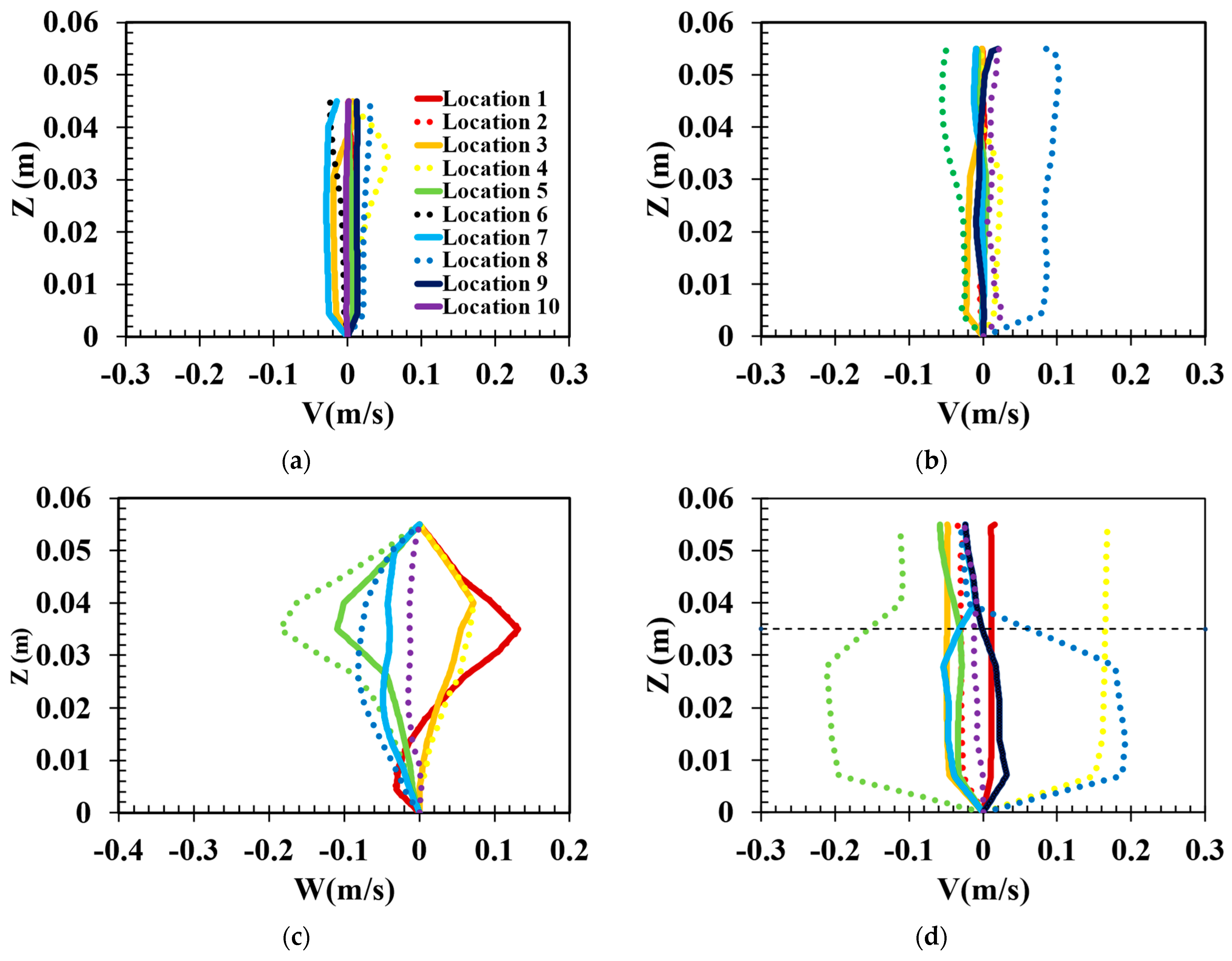
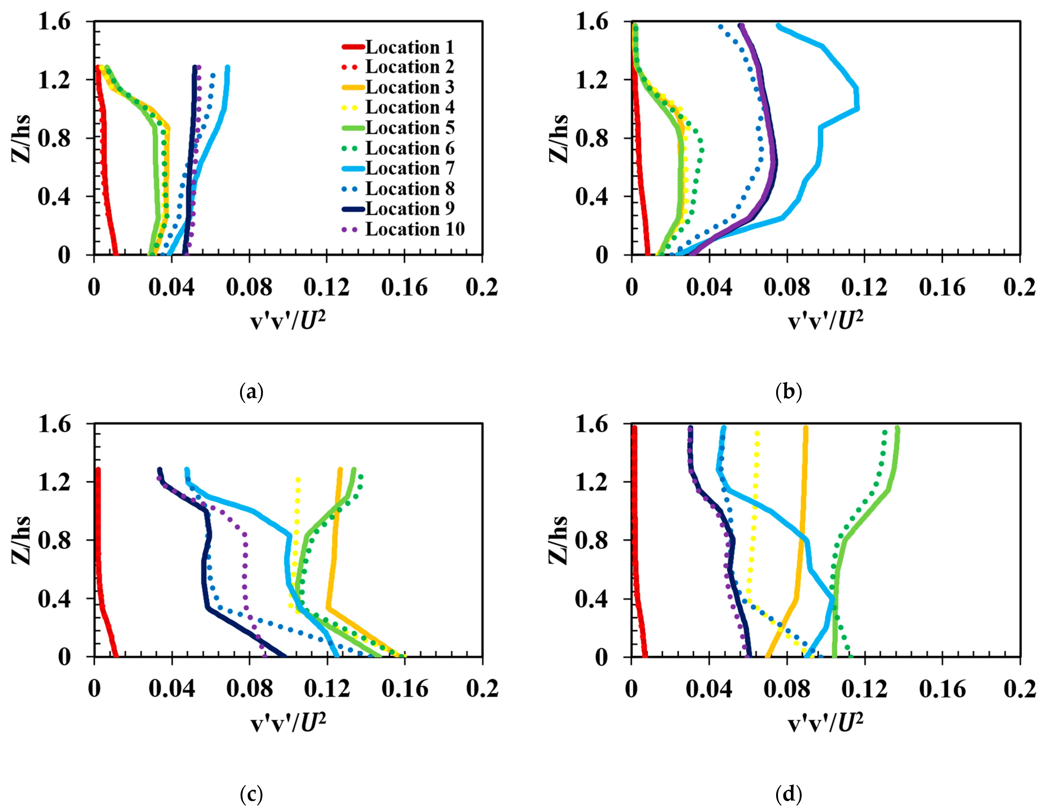
The cross-streamwise velocity component (v) of all four cases is represented in Figure 6a–d. It is evident from Figure 6 that the cross-streamwise velocities are very low upstream (locations 1–2) and downstream (locations 9–10) of the trees during all cases because there is less cross-streamwise movement at these locations, The values of the cross-streamwise velocities are positive and negative at those locations that lie inside the trees, due to the maximum lateral movement and small turbulence caused by the trees.
The plot of cross-streamwise velocities is almost constant from bed to top at locations that are located inside the tall trees (locations 7–10 in cases 1–2 and locations 1–4 in cases 3–4). The reason for this is the persistent resistance presented by the taller trees all the way to their crowns, whereas an inflection point near the tops of the short trees can be seen at locations lying inside or surrounding the short trees (locations 1–4 in cases 1–2 and locations 7–10 in cases 3–4). Within the short trees’ cylinders (Z ≤ 0.035 m), smaller fluctuations in velocity are observed due to the presence of turbulence. The overall velocities at points located in the free streamwise region (locations 2, 4, 6, 8, and 10) are comparatively higher than those at points locating in line with the trees (locations 1, 3, 5, 7, and 9) in all cases.

4.1.3. Vertical Distribution of Depthwise Velocity (w)

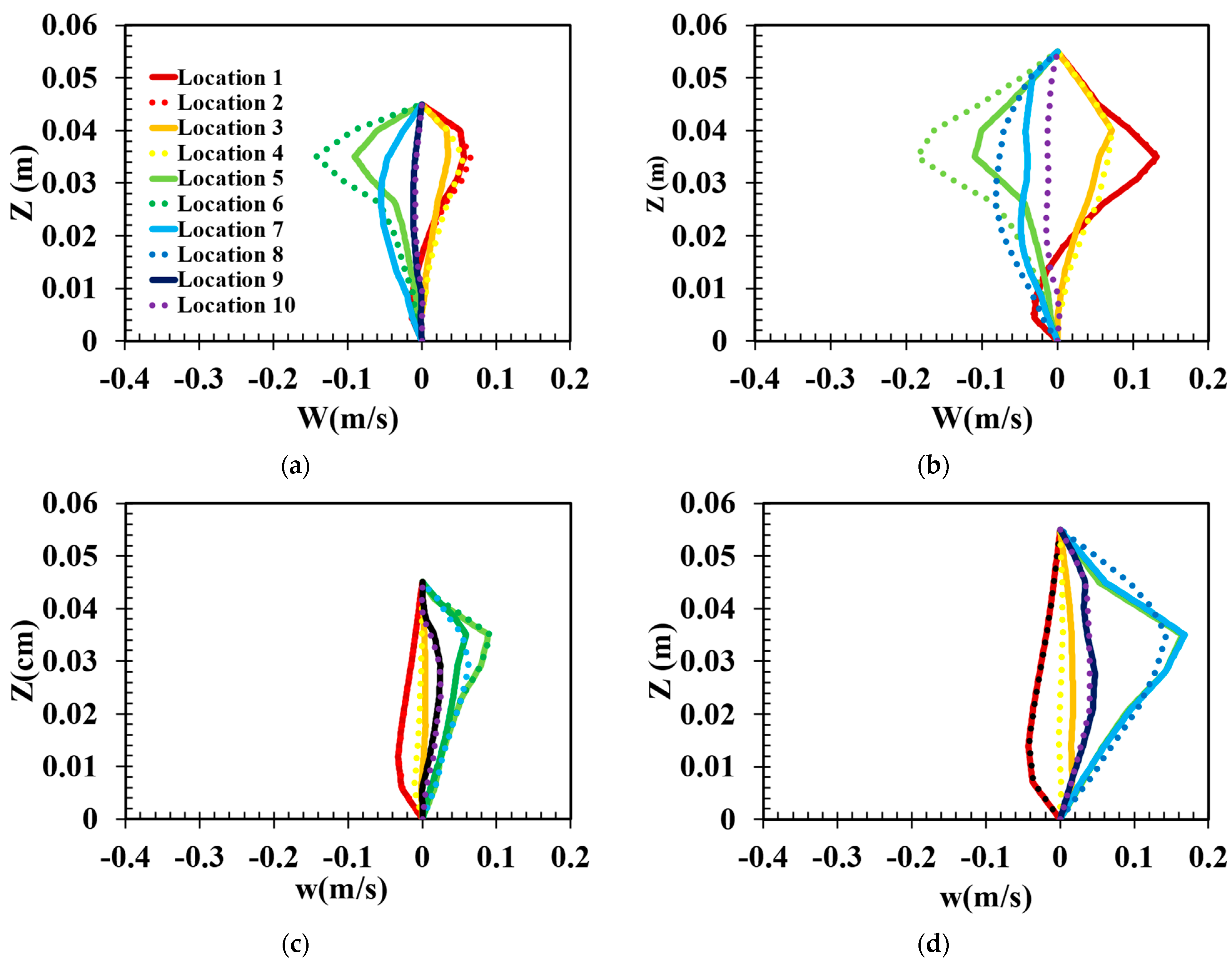
The trend of depthwise velocities (w) in case 1 is similar to that in case 2, while case 3 is similar to case 4 at specific locations, as shown in Figure 7a–d. It can be seen from the plots of depthwise velocities that a sharp inflection in depthwise velocity with maximum positive (indicating upward flow velocity) or negative values (representing downward flow motion) was visible near the tops of the short trees at all those locations lying inside or surrounding the layer of short trees.
The motion of flow was upward at locations 1–4 near the tops of the short trees in cases 1–2 (Figure 6a,b), while the negative maximum values in the plots of velocities at locations 5–8 in cases 1 and 2 indicate the downward movement of flow at these locations. The behavior of depthwise velocities at locations 9-10 was almost constant up to the tops of the trees.
Meanwhile, the velocities at locations 1–4 in cases 3–4 were almost constant from bed to top.
Similarly, an interesting trend of velocity was observed at locations 5–8 in cases 3 and 4 (Figure 6c,d), because these locations were amongst the short trees. The vertical velocities were increased along with the water depth and reached their maximum positive values inside the short trees (Z < 0.035 m), and above Z ≥ 0.035 m the velocities tended to decrease up to the free surface.
The increasing pattern of velocities inside the short trees is a depiction of upward flow, while the decreasing pattern of velocities after Z ≥ 0.035 m represents the downward direction of flow. From the plots of locations 9 and 10, it is visible that the velocities at these locations are near to zero and constant up to the top of a free surface, indicating no vertical movement of flow at these locations.
From the above discussion, it can be concluded that the upward and downward movement of flow was observed upstream and downstream of the trees, respectively, whereas the behavior of velocities amongst the taller trees was almost constant from bed to top.

4.2. Vertical Distribution of Reynolds Stresses

To learn more about turbulence, the Reynolds stresses in the computational model were calculated. Figure 8 and Figure 9 illustrate the vertical profiles of the computed Reynolds stresses (u’u’, v’v’, w’w’, and u’w’) at various specified locations, where u’, v’, and w’ represent changes in the streamwise, lateral, and vertical directions of the velocity component, respectively. Reynolds stresses, normalized by U2, are shown on the X-axis, while flow depth, normalized by hs (the smaller trees’ height), is shown on the Y-axis.

4.2.1. Normal Stresses (u’u’)

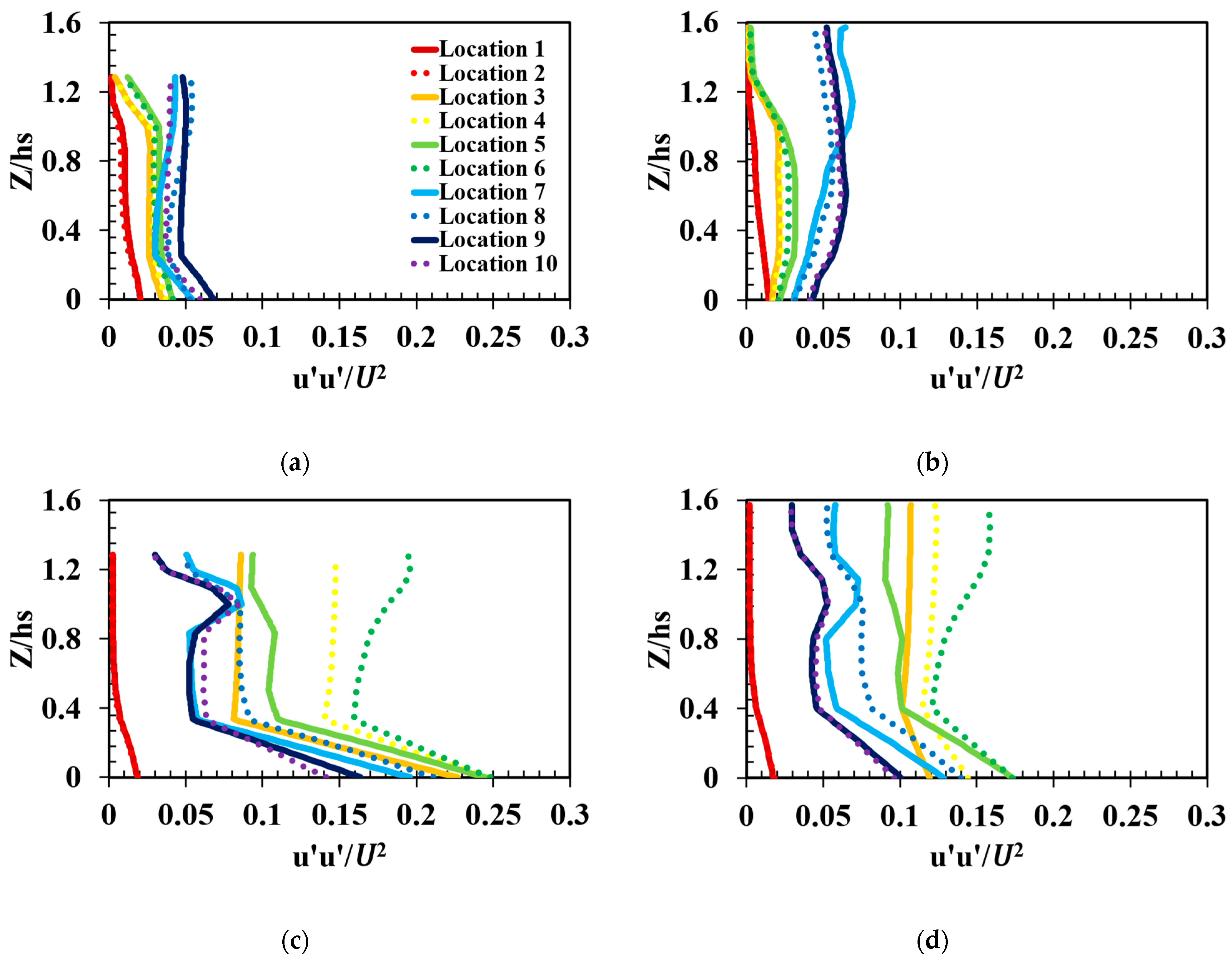
It is visible form Figure 8a–d that the normal stresses (u’u’) are maximal near the bed at all locations during all cases. The normal stresses are relatively higher at locations 7–10, which lie inside and downstream of the taller layers as compared to locations 3–6 in the smaller layers in cases 1–2, and at locations 3–6 (located in the taller layers) as compared to locations 7–10 (located in the smaller layers) in cases 3–4. The Reynolds normal stresses are almost constant form the beds to the tops of the cylinders at those points that are located amongst the taller trees (i.e., locations 1–4 in cases 3–4, and locations 7–10 in cases 1–2). The plots of locations that are located amongst the short trees (locations 1–4 in cases 1–2; locations 7–10 in cases 3–4) consist of three different behaviors: initially, normal stresses are very low near the bed up to a certain flow depth; in the second zone of the plots these stresses become constant before the tops of the trees, while in the third zone of the plots inflection points occur, where sharp variation is visible near the tops of the trees (Z/hs = 1) due to the exchange of momentum between flow layers.

4.2.2. Normal Stresses (v’v’)

In all cases, the normal stresses (v’v’) are minimal at upstream locations 1–2 as compared to downstream, and they remain constant up to the tops of the trees, as shown in Figure 9a–d. A sharp inflection point is visible in plots of normal stresses at the interface of trees and flow, due to the high turbulence at all those locations lying inside and downstream of the submerged trees (locations 3–6 in cases 1–2; locations 7–10 in cases 3–4). In contrast, the normal stresses (v’v’) are relatively higher at those locations lying inside the tall trees (i.e., locations 7–10 in cases 1–2; locations 3–6 in cases 3–4) as compared to the locations of the short trees. The stresses inside the short trees in the vegetated zone (Z/hs < 1) are higher as compared to the unvegetated zone (Z/hs > 1), while the increasing pattern of (v’v’) normal stresses inside the tree patches (i.e., Z/hs ≤ 0.8831 below the tops of submerged trees) at specified points can be arranged as 2 < 1 < 5 < 4 < 6 < 3 < 8 < 9 < 10 < 7. Meanwhile, the plot of normal stresses v’v’ depicts that the overall (v’v’) normal stresses near the tops of the short trees (i.e., Z/hs ≥ 0.8831) follows the pattern 2 < 1 < 5 < 4 < 6 < 3 < 9 <10 < 8 < 7. The overall stresses in case 2 are larger as compared to case 1 at specified points.

4.2.3. Normal Stresses (w’w’)

The normal stresses, w’w’ are minimal at locations 1–2 as compared to downstream and all other locations in all cases (Figure 10a,d), because these locations lie directly upstream of the trees, where the hindrance due to trees and backwater reflection occurs. The plot of these locations (1–2) in cases 3–4 is almost constant from bed to top, because in these cases resistance continues up to the top along with the tall trees, whereas the plot of locations 1–2 in cases 1–2 shows different behavior—initially it is relatively constant, while the inflection point is visible near the tops of submerged trees due to momentum exchange between the flow layers. The overall Reynolds normal stresses are relatively larger at those points located amongst the tall trees (i.e., locations 7–10 in cases 1–2; locations 3–6 in cases 3–4) as compared to those lying amongst the short trees.

4.2.4. Reynolds Shear Stresses (u’w’)

Figure 11 depicts the vertical distribution of Reynolds shear stresses for all cases. In all four cases, the plotted Reynolds shear stresses consist of three parts. In the first portion (Z/hs < 020), in cases 1–2 (Figure 11a,b), the stresses near the bed are greater at locations 7–10 as compared to the other locations, and the value of the stresses is positive, with a decreasing trend up to Z/hs < 0.20, whereas in cases 3-4 (Figure 11c,d) the stresses are maximally negative at all locations in the first portion of the plot (Z/hs < 0.20). Meanwhile, in the second portion, the stresses are almost constant from bed to top at locations 9-10 (located downstream of the taller layer) in cases 1–2 and locations 1–4 in cases 3–4. In the third portion of the plot, a sharp inflection in the Reynolds shear stresses can be observed at the interface of the short trees at locations 3–6 in cases 1–2 and locations 5–10 in cases 3–4. From the above discussion, it can be concluded that the Reynolds shear stresses were maximal amongst the trees of the second patch (taller trees in cases 1–2 and shorter trees in cases 3–4) near the bed (i.e., z/hs < 0.20).

4.3. Distribution of Turbulence Kinetic Energy

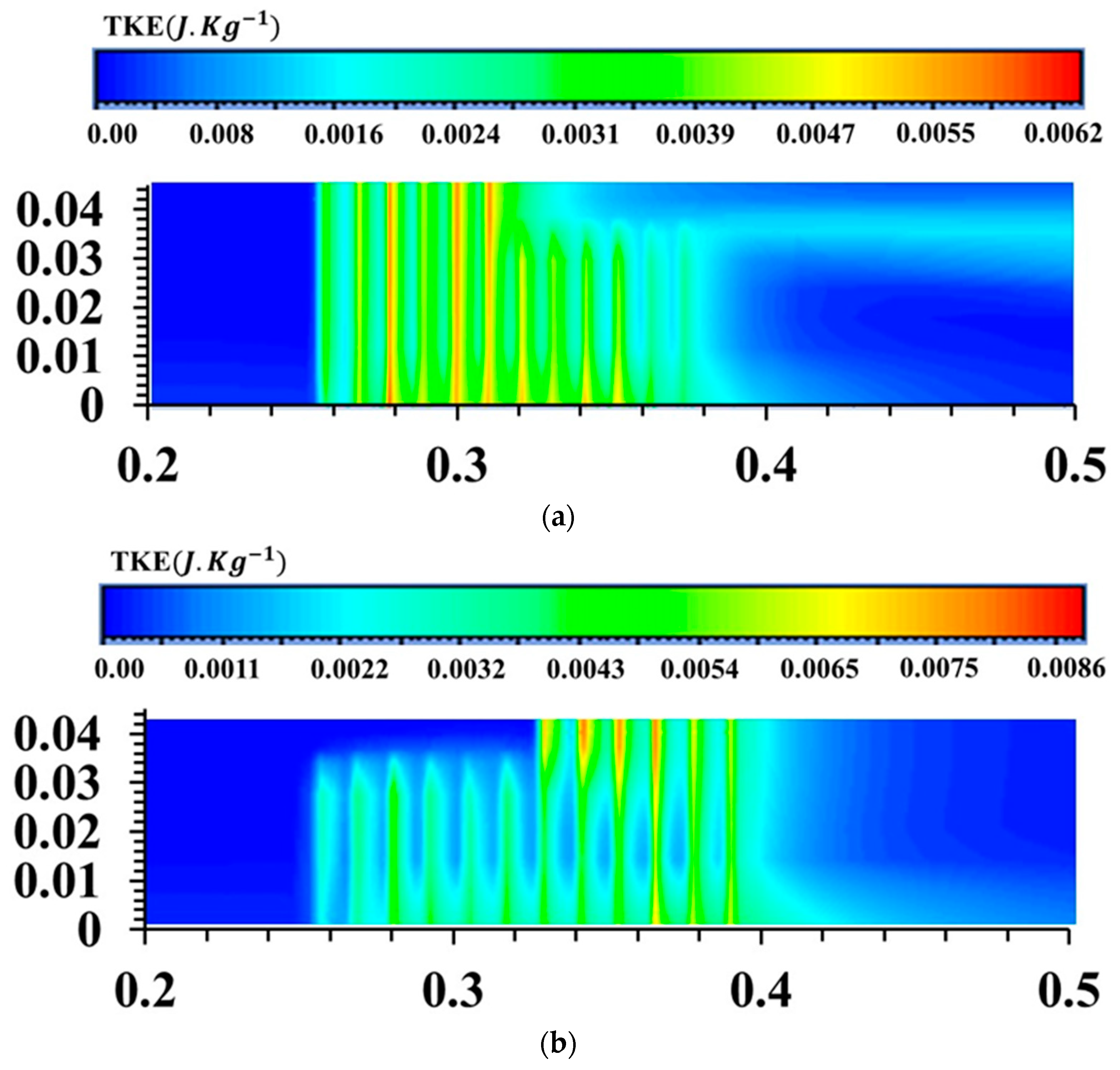
The contour plots in Figure 12a,b show the distribution of kinetic energy in turbulence along longitudinal section 1 for cases 1 and 3, respectively. The X-axis represents the channel’s length, while the Y-axis represents the water’s depth along the channel (Z). In cases 1 and 3, there is a distinct variation in the turbulence kinetic energy values between the patch of trees and the regions upstream and downstream of it. The magnitude of the turbulence kinetic energy within the patch of trees was substantially bigger than the magnitude of the turbulence kinetic energy upstream and downstream of the patch of trees. As a direct result of this, the TKE significantly increased in the region that encompassed the patch of trees, illustrating a correlation with the data presented in an earlier study [32]. The turbulence kinetic energy of the patch of trees increased by a percentage difference that ranged from 46 to 70% for case 1 and from 38 to 57% for case 3, when contrasted with the upstream and downstream regions without any trees. This is in stark contrast to the lack of trees that may be found in the regions that are upstream and downstream. The increased magnitude of turbulence kinetic energy that was seen within the patch of trees was the result of the resistance that was supplied by the tree cylinders. This was the source of the increased magnitude of turbulence kinetic energy. This resistance was not present in the locations that were either upstream or downstream of the point of study. Because of the continuous resistance of the cylinders, the behavior of the turbulence kinetic energy contained within the tall and short trees remained virtually the same from the bottom to the top of the cylinders, although it was observed that there was a sudden shift in the turbulence kinetic energy directly above the short trees in cases 1 and 3. The magnitude of the turbulence kinetic energy directly above the short trees was significantly lower when compared to the turbulence kinetic energy found inside the patch of trees. Based on these findings, it appears that the patch of trees contains a greater amount of turbulence within the trees.

4.4. Turbulence Eddy Dissipation Rate

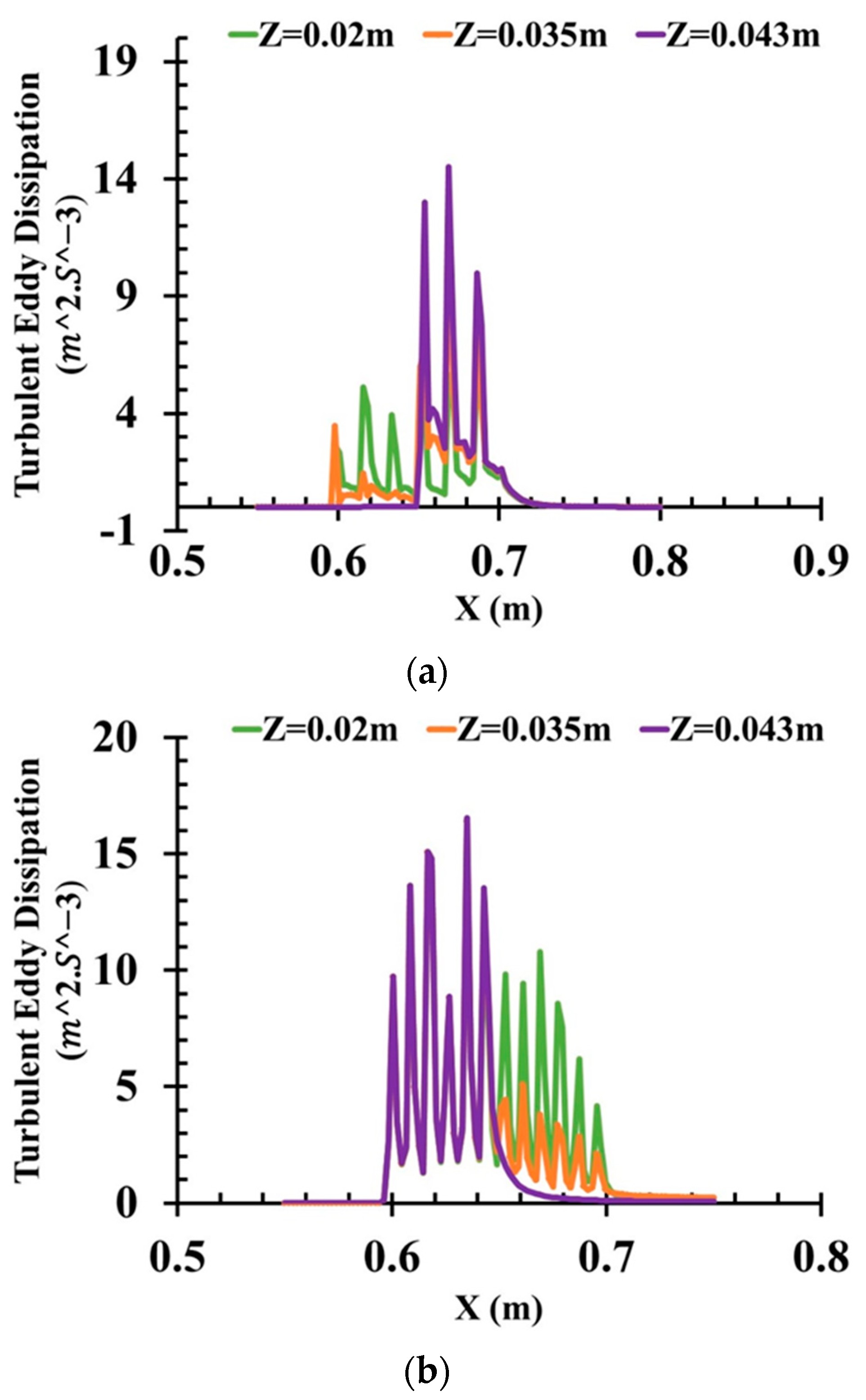
Figure 13a,b depict the profile of the turbulence eddy dissipation rate inside the tree patch (Z/hs < 1), at the tops of the short trees (Z/hs = 1), above the short trees (Z/hs > 1), and along the centerline of the tree patch (Section 1) for case 1 (short and tall trees) and case 3 (tall and short trees), respectively. The kinetic energy of the flow turbulence relates to the eddies, and this turbulence energy is lost as a result of the larger eddies dissipating into smaller ones at a faster rate than it is converted to heat by the viscous forces. The trend of the turbulence eddy dissipation rate is quite similar to that of the turbulence kinetic energy in many respects, as shown in Figure 12. A distinct contrast is clearly visible between the tree region and the region that does not have trees, i.e., upstream and downstream. When comparing cases 1 and 3, the behavior of the eddy dissipation rate is essentially same across a range of flow depths—specifically at Z/hs < 1, Z/hs = 1, and Z/h > 1. At the locations upstream and the downstream of the patch of trees, the turbulent eddy dissipation was essentially non-existent; as the flow proceeded through the tree region, there was a sawtooth pattern seen in the rising trends of the energy distribution that was being lost. In cases 1 and 3, the continuous flow obstruction up to the tops of the trees caused the magnitude of the eddy dissipation rate to be higher inside the patch of tall trees as compared to the short trees.

5. Conclusions

Detailed knowledge and comparison between flow characteristics along the flow depth in a horizontal double layers of trees with varying arrangements of short submerged trees ( P S ) and tall emergent trees ( P t ) have still not been investigated. Hence, the numerical analysis of flow structure through different arrangements of horizontal double layers of trees was carried out with the application of the numerical code Fluent (ANSYS) and Reynolds stress modeling (RSM) to replicate the vertical profiles of velocities, Reynolds stresses, turbulence kinetic energy, and turbulence eddy dissipation rate. The current computational study effectively computed the appropriate results of internal flow properties along the flow depth, and it showed great accordance with experimental outcomes of [19]. The main findings acquired from this study are as follows:
  • In all cases, the mean streamwise (u’), lateral (v’), and vertical (w’) velocity profiles consisted of a sharp inflection point in the zone 0.035 m < z < 0.04 m at all those locations lying inside, upstream, and downstream of the short trees ( P S ). This was due to the maximum generation of vortices that gave rise to the momentum transfer between the overlying flow and the tops of the shorter trees, which indicatively represent a gradient of velocity in this zone. There was an approximate 31–65% increase in the streamwise velocities at locations 1-6 in cases 1–2 and a 54–77% increase at locations 7–10 in cases 3–4 in the unvegetated zone (z > 0.035 m) compared to the vegetated zone (z < 0.035 m) below the short trees. In contrast, the trend of streamwise velocities amongst the taller trees was almost constant from bed to top due to continuous resistance up to tops of the tall trees.
  • In all cases, the normal stresses were higher at those locations lying amongst the taller trees and almost constant from bed to top as compared to the locations of submerged trees, where sharp inflection points were observed at the interface of the submerged trees due momentum exchange between the flow layers. Meanwhile, the normal stresses were lesser directly downstream of the cylinders at locations 3-7 as compared to locations 4 and 8.
  • The magnitude of the turbulence kinetic energy was significantly larger inside the short and tall tree cylinders as compared to the unvegetated regions, i.e., the upstream and downstream regions. Similarly, the production of turbulence kinetic energy was approximately 50% and 70% greater inside the tree region (Z < 0.035) as compared to above the shorter trees during cases 1–2 and cases 3–4, respectively.
  • The sawtooth pattern in the turbulence eddy dissipation rate was noticed in all cases inside the tree region, while a greater eddy dissipation rate was observed amongst the tall trees as compared to the short trees. This was due to the significantly higher continuous flow resistance offered by the tall trees up to the tops of the taller tree cylinders.
The purpose of this research was to examine the potential of a horizontal double layer of trees (HDLT) made up of both short and tall layers, as a defense mechanism against tsunami floods in inland areas. The outcomes of the present numerical study clearly show the effectiveness of a horizontal double layer of trees arranged in patches of short and tall trees to withstand the spread of tsunamis and floods. The horizontal double layer of trees arranged with short upstream and tall downstream trees was more favorable in terms of greater flow resistance and better dissipation of turbulence energy as compared to the arrangement with tall upstream and short downstream trees. Hence, this particular pattern of HDLT has the potential to be very useful during times of high flow and floods. In order to facilitate future research, it is possible to presuppose a variety of flow depths and discharges in order to examine the effects of various patch combinations on the flow structures. In addition, more measurement positions in the streamwise direction (as well as in other directions) should be sought, in order to study these variances in greater detail. Moreover, additional experimental research is required to further investigate the phenomenon and the consequent flow pattern of scouring behind the downstream forest under movable bed conditions and larger flows.

Author Contributions

Conceptualization, N.T.; Methodology, F.M.A.; Software, F.M.A. and A.; Validation, F.M.A.; Investigation, F.M.A. and A.; Writing—original draft, F.M.A. and A.; Writing—review & editing, F.M.A.; Visualization, N.T. and A.; Supervision, N.T. All authors have read and agreed to the published version of the manuscript.

Funding

This research received no external funding.

Acknowledgments

The authors acknowledge the support of the MEXT scholarship (Fakhar Muhammad Abbas and Amina) from the Japanese Ministry of Education, Culture, Sports, Science, and Technology (Monbukagakusho).

Conflicts of Interest

The authors declare no conflict of interest.

References

  1. Mori, N.; Takahashi, T. The 2011 Tohoku Earthquake Tsunami Joint Survey Group, 2012. Nationwide post event survey and analysis of the 2011 Tohoku earthquake tsunami. Coast Eng. J. 2011, 52, 1250001-1–1250001-27. [Google Scholar]
  2. Danielsen, F.; Sorensen, M.K.; Olwig, M.F.; Selvam, V.; Parish, F.; Burgess, N.D.; Hiraishi, T.; Karunagaran, V.M.; Rasmussen, M.S.; Hansen, L.B.; et al. The Asian tsunami: A protective role for coastal vegetation. Science 2005, 310, 643. [Google Scholar] [CrossRef] [Green Version]
  3. Suppasri, A.; Koshimura, S.; Imai, K.; Mas, E.; Gokon, H.; Muhari, A.; Imamura, F. Developing tsunami fragility curves from the surveyed data of the 2011 Great East Japan tsunami in Sendai and Ishinomaki Plains. Coast. Eng. J. 2012, 54, 1250008-1–1250008-16. [Google Scholar] [CrossRef]
  4. Nateghi, R.; Bricker, J.D.; Guikema, S.D.; Bessho, A. Statistical analysis of the effectiveness of seawalls and coastal forests in mitigating tsunami impacts in Iwate and Miyagi prefectures. PLoS ONE 2016, 11, e0158375. [Google Scholar] [CrossRef] [PubMed] [Green Version]
  5. Fraser, S.; Raby, A.; Pomonis, A.; Goda, K.; Chian, S.C.; Macabuag, J.; Offord, M.; Saito, K.; Sammonds, P. Tsunami damage to coastal defences and buildings in the March 11th, 2011 Mw 9.0 Great East Japan earthquake and tsunami. Bull. Earthq. Eng. 2013, 11, 205–239. [Google Scholar] [CrossRef]
  6. Osti, R.; Tanaka, S.; Tokioka, T. The importance of mangrove forest in tsunami disaster mitigation. Disasters 2009, 33, 203–213. [Google Scholar] [CrossRef] [PubMed]
  7. Kathiresan, K.; Rajendran, N. Coastal mangrove forests mitigated tsunami. Estuar. Coast. Shelf Sci. 2005, 65, 601–606. [Google Scholar] [CrossRef]
  8. Yanagisawa, H.; Koshimura, S.; Goto, K.; Miyagi, T.; Imamura, F.; Ruangrassamee, A.; Tanavud, C. The reduction effects of mangrove forest on a tsunami based on field surveys at Pakarang Cape, Thailand and numerical analysis. Estuar. Coast. Shelf Sci. 2009, 81, 27–37. [Google Scholar] [CrossRef]
  9. Yanagisawa, H.; Koshimura, S.; Miyagi, T.; Imamura, F. Tsunami damage reduction performance of a mangrove forest in Banda Aceh, Indonesia inferred from field data and a numerical model. J. Geophys. Res. 2010, 115, C06032. [Google Scholar] [CrossRef] [Green Version]
  10. Takemura, T.; Tanaka, N. Flow structures and drag characteristics of a colony type emergent roughness model mounted on a flat plate in uniform flow. Fluid Dyn. Res. 2007, 39, 694–710. [Google Scholar] [CrossRef]
  11. Huai, W.; Wang, W.; Hu, Y.; Zeng, Y.; Keith, Z.Y. Analytical model of the mean velocity distribution in an open channel with double-layered rigid vegetation. Adv. Water Resour. 2014, 69, 106–113. [Google Scholar] [CrossRef]
  12. Lima, P.; Janzen, J.; Nepf, H. Flow patterns around two neighbouring patches of emergent vegetation and possible implications for deposition and vegetation growth. Environ. Fluid Mech. 2015, 15, 881–898. [Google Scholar] [CrossRef]
  13. Shimizu, Y.; Tsujimoto, T. Numerical analysis of turbulent open-channel flow over vegetation layer using a k-ɛ turbulence model. J. Hydrosci. Hydraul. Eng. 1994, 11, 57–67. [Google Scholar]
  14. Singh, P.; Rahimi, H.R.; Tang, X. Parameterization of the modeling variables in velocity analytical solutions of open-channel flows with double-layered vegetation. Environ. Fluid Mech. 2019, 19, 765–784. [Google Scholar] [CrossRef]
  15. Poggi, D.; Porporato, A.; Ridolfi, L.; Albertson, J.D.; Katul, G.G. The effect of vegetation density on canopy sub-layer turbulence. Bound. Layer Meteorol. 2004, 111, 565–587. [Google Scholar] [CrossRef]
  16. Raupach, M.R.; Shaw, R.H. Averaging procedures for flow within vegetation canopies. Bound. -Layer Meteorol. 1982, 22, 79–90. [Google Scholar] [CrossRef]
  17. Anjum, N.; Ghani, U.; Pasha, G.A.; Latif, A.; Sultan, T.; Ali, S. To investigate the flow structure of discontinuous vegetation patches of two vertically different layers in an open channel. Water 2018, 10, 75. [Google Scholar] [CrossRef] [Green Version]
  18. Pu, J.H.; Hussain, A.; Guo, Y.K.; Vardakastanis, N.; Hanmaiahgari, P.R.; Lam, D. Submerged flexible vegetation impact on open channel flow velocity distribution: An analytical modelling study on drag and friction. Water Sci. Eng. 2019, 12, 121–128. [Google Scholar] [CrossRef]
  19. Kundu, P.; Kumar, V.; Hoarau, Y. Numerical simulation and analysis of fluid flow hydrodynamics through a structured array of circular cylinders forming porous medium. Appl. Math. Model. 2016, 40, 9848–9871. [Google Scholar] [CrossRef]
  20. Wang, W.; Huai, W.X.; Gao, M. Computation of flow structure through double layer vegetation. Math. Comput. Methods Sci. Eng. 2014, 132–136. [Google Scholar]
  21. Ghani, U.; Anjum, N.; Pasha, G.A.; Ahmad, M. Numerical investigation of the flow characteristics through discontinuous and layered vegetation patches of finite width in an open channel. Environ. Fluid Mech 2019, 19, 1469–1495. [Google Scholar] [CrossRef]
  22. Xiaohui, S.; Li, C.W. Large eddy simulation of free surface turbulent flow in partly vegetated open channels. Int. J. Numer. Methods Fluids 2002, 39, 919–937. [Google Scholar] [CrossRef]
  23. Yan, C.; Nepf, H.M.; Huang, W.X.; Cui, G.X. Large eddy simulation of flow and scalar transport in a vegetated channel. Environ. Fluid Mech. 2017, 17, 497–519. [Google Scholar] [CrossRef]
  24. Wu, W.; Shields, F.D., Jr.; Bennett, S.J.; Wang, S.S.Y. A depth averaged two-dimensional model for flow, sediment transport, and bed topography in curved channels with riparian trees. Water Resour. Res. 2005, 41, 1–15. [Google Scholar] [CrossRef]
  25. Tanaka, N. Numerical Investigation of 3D Flow Properties around Finite Emergent Trees by Using the Two-Phase Volume of Fluid (VOF) Modeling Technique. Fluids 2022, 7, 175. [Google Scholar] [CrossRef]
  26. Zhao, F.; Huai, W. Hydrodynamics of discontinuous rigid submerged trees patches in open-channel flow. J. Hydro-Environ. Res. 2016, 12, 148–160. [Google Scholar] [CrossRef]
  27. Harada, K.; Kawata, Y. Study on tsunami reduction effect of coastal forest due to forest growth. Ann. Disaster Prev. Res. Inst. 2005, 48C, 161–165. [Google Scholar]
  28. Hiraishi, T.; Harada, K. Greenbelt tsunami prevention in South-Pacific region. Rep. Port Airpt. Res. Inst. 2003, 42, 23. [Google Scholar]
  29. Tanaka, N. Variation of tree crown height effects on flow behavior around finite vegetation. J. Appl. Water Eng. Res. 2022, 1–13. [Google Scholar] [CrossRef]
  30. Tanaka, N. Experimental Study to Evaluate the Effectiveness of the Variation in Crown Portion of a Tree on the Flow Properties Considering the Finite Length Forest. Int. J. Civ. Eng. 2022, 20, 1461–1478. [Google Scholar] [CrossRef]
  31. Ishigaki, A.; Higashi, H.; Sakamoto, S.; Shibahara, S. The Great East–Japan earthquake and devastating tsunami: An update and lessons from the past great earthquakes in Japan since 1923. Tohoku J. Exp. Med. 2013, 229, 287–299. [Google Scholar] [CrossRef] [Green Version]
  32. Samarakoon, M.B.; Tanaka, N.; Iimura, K. Improvement of effectiveness of existing Casuarina equisetifolia forests in mitigating tsunami damage. J. Environ. Manag. 2013, 114, 105–114. [Google Scholar] [CrossRef] [PubMed]
  33. Liu, D.; Diplas, P.; Hodges, C.C.; Fairbanks, J.D. Hydrodynamics of flow through double layer rigid vegetation. Geomorphology 2010, 116, 286–296. [Google Scholar] [CrossRef]
  34. Roulund, A.; Sumer, B.M.; Fredsfe, J.; Michelsen, J. Numerical and experimental investigation of flow and scour around a circular pile. J. Fluid Mech. 2005, 534, 351–401. [Google Scholar] [CrossRef]
  35. Anjum, N.; Tanaka, N. Numerical investigation of velocity distribution of turbulent flow through vertically double-layered vegetation. Water Sci. Eng. 2019, 12, 319–329. [Google Scholar] [CrossRef]
  36. Choi, S.U.; Kang, H. Reynolds stress modeling of vegetated open-channel flows. J. Hydraul Res. 2004, 42, 3–11. [Google Scholar] [CrossRef]
  37. Fritz, H.M.; Borrero, J.C.; Synolakis, C.E.; Yoo, J. 2004 Indian Ocean tsunami flow velocity measurements from survivor videos. Geophys. Res. Lett. 2006, L33, 24605. [Google Scholar] [CrossRef]
  38. Tanaka, N.; Sasaki, Y.; Mowjood, M.I.M.; Jinadasa, K.B.S.N.; Homchuen, S. Coastal trees structures and their functions in tsunami protection: Experience of the recent Indian Ocean tsunami. Lands. Ecol. Eng. 2007, 3, 33–45. [Google Scholar] [CrossRef]
  39. Jayatissa, L.P.; Dahdouh Guebas, F.; Koedam, N. A review of the floral composition and distribution of mangroves in Sri Lanka. Bot. J. Linn. Soc. 2002, 138, 29–43. [Google Scholar] [CrossRef]
  40. Wolanski, E.; Jones, M.; Bunt, S.J. Hydrodynamics of a tidal creek-mangrove swamp system. Aust. J. Mar. Freshw. Res. 1980, 31, 431–450. [Google Scholar] [CrossRef]
  41. Zheng, J.H.; Wang, J.C.; Zhou, C.Y.; Zhao, H.J.; Sang, S. Numerical simulation of typhoon-induced storm surge along Jiangsu coast, Part II: Calculation of storm surge. Water Sci. Eng. 2017, 10, 8–16. [Google Scholar] [CrossRef]
  42. Fluent Inc User’s Guide; Release 19.2; ANSYS, Inc.: Canonsburg, PA, USA, 2020.
  43. Rahimi, H.R.; Tang, X.; Singh, P. Experimental and numerical study on impact of double layer vegetation in open channel flows. J. Hydrol. Eng. 2020, 25, 04019064. [Google Scholar] [CrossRef]
  44. Righetti, M.; Armanini, A. Flow resistance in open channel flows with sparsely distributed bushes. J. Hydrol. 2002, 269, 55–64. [Google Scholar] [CrossRef]
  45. Liu, D.; Diplas, P.; Fairbanks, J.D.; Hodges, C.C. An experimental study of flow through rigid vegetation. J. Geophys. Res. 2008, 113, 1–16. [Google Scholar] [CrossRef]
  46. Yan, X.; Wai, W.O.; Li, C. Characteristics of flow structure of free-surface flow in a partly obstructed open channel with vegetation patch. Environ. Fluid Mech. 2016, 16, 807–832. [Google Scholar] [CrossRef]
Figure 1. Experimental geometry of [34], where the top view of the geometry is shown and three selected positions are selected (P1, P2, P3).
Mathematics 11 00712 g001
Figure 2. Comparison between the experimental results of [33] and the computed results of (a) velocity profiles and (b) turbulence intensity profiles.
Mathematics 11 00712 g002aMathematics 11 00712 g002b
Figure 3. (a,b) Schematic diagram of the numerical domain, along with specific locations for cases 1–2 and 3–4, respectively.
Mathematics 11 00712 g003
Figure 4. Spacing between cylinders.
Mathematics 11 00712 g004
Figure 5. (ad) The simulated results of mean streamwise velocity profiles (u) at specified locations: (a) case 1; (b) case 2; (c) case 3; (d) case 4.
Mathematics 11 00712 g005aMathematics 11 00712 g005b
Figure 6. (ad) The simulated results of the lateral velocity profiles (v) at specified locations: (a) case 1; (b) case 2; (c) case 3; (d) case 4.
Mathematics 11 00712 g006
Figure 7. (ad) The simulated results of vertical velocity profiles (w) at specified locations: (a) case 1; (b) case 2; (c) case 3; (d) case 4.
Mathematics 11 00712 g007
Figure 8. (ad) The vertical profiles of normal stresses (u’u’) at specified locations: (a) case 1; (b) case 2; (c) case 3; (d) case 4.
Mathematics 11 00712 g008
Figure 9. (ad) The vertical profiles of normal stresses (v’v’) at specified locations: (a) case 1; (b) case 2; (c) case 3; (d) case 4.
Mathematics 11 00712 g009
Figure 10. (ad) The vertical profiles of normal stresses (w’w’) at specified locations: (a) case 1; (b) case 2; (c) case 3; (d) case 4.
Mathematics 11 00712 g010
Figure 11. (ad) The vertical profiles of shear stresses (−u’w’) at specified locations: (a) case 1; (b) case 2; (c) case 3; (d) case 4.
Mathematics 11 00712 g011
Figure 12. Longitudinal contour plot distribution of turbulence kinetic energy (TKE): (a) case 1; (b) case 3.
Mathematics 11 00712 g012
Figure 13. Longitudinal distribution of turbulence eddy dissipation rate: (a) case 1; (b) case 3.
Mathematics 11 00712 g013
Table 1. Hydraulic conditions of the numerical model.
Case No.Vegetation ConfigurationZ (cm)Vegetation Density (Cylinders/m2)FrCylinder Arrangement
1Short Patch + Tall Patch4.51.220.65Staggered
2Short Patch + Tall Patch5.51.220.68Staggered
3Tall Patch + Short Patch4.51.220.65Staggered
4Tall Patch + Short Patch5.51.220.68Staggered
Note: Z is the water depth; G/d is the density of the trees; U represents the initial velocity.
Disclaimer/Publisher’s Note: The statements, opinions and data contained in all publications are solely those of the individual author(s) and contributor(s) and not of MDPI and/or the editor(s). MDPI and/or the editor(s) disclaim responsibility for any injury to people or property resulting from any ideas, methods, instructions or products referred to in the content.