A Combinatorial Approach to Study the Nordhaus–Guddum-Type Results for Steiner Degree Distance

Abstract

In 1994, Dobrynin and Kochetova introduced the concept of degree distance $DD(\Gamma )$ of a connected graph $\Gamma$. Let $d_{\Gamma }\left(S\right)$ be the Steiner k-distance of $S\subseteq V(\Gamma )$. The Steiner Wiener k-index or k-center Steiner Wiener index${SW}_k(\Gamma )$ of $\Gamma$ is defined by ${SW}_k(\Gamma )={\sum }_{\stackrel{S\subseteq V(\Gamma )}{\left|S\right|=k}}{d}_{\Gamma }\left(S\right).$ The k-center Steiner degree distance${SDD}_k(\Gamma )$ of a connected graph $\Gamma$ is defined by ${SDD}_k(\Gamma )={\sum }_{\stackrel{S\subseteq V(\Gamma )}{\left|S\right|=k}}\left[{\sum }_{v\in S}de{g}_{\Gamma }\left(v\right)\right]d_{\Gamma }\left(S\right)$, where $de{g}_{\Gamma }\left(v\right)$ is the degree of the vertex v in $\Gamma$. In this paper, we consider the Nordhaus–Gaddum-type results for ${SW}_k(\Gamma )$ and ${SDD}_k(\Gamma )$. Upper bounds on ${SW}_k(\Gamma )+{SW}_k\left(\overline{\Gamma }\right)$ and ${SW}_k(\Gamma )·{SW}_k\left(\overline{\Gamma }\right)$ are obtained for a connected graph $\Gamma$ and compared with previous bounds. We present sharp upper and lower bounds of ${SDD}_k(\Gamma )+{SDD}_k\left(\overline{\Gamma }\right)$ and ${SDD}_k(\Gamma )·{SDD}_k\left(\overline{\Gamma }\right)$ for a connected graph $\Gamma$ of order n with maximum degree $\Delta$ and minimum degree $\delta$. Some graph classes attaining these bounds are also given.

1. Introduction

In this paper, all the graphs are simple and connected. We refer to [1] for graph theoretical notation and terminology not described here. For a graph $\Gamma$, let $V(\Gamma )$, $E(\Gamma )$, $\overline{\Gamma }$ and $e(\Gamma )=\left|E\right(\Gamma \left)\right|$ denote the set of vertices, the set of edges, the complement and the size of $\Gamma$, respectively. Let $de{g}_{\Gamma }\left(u\right)$ be the degree of the vertex $u\in V(\Gamma )$. The maximum degree of a vertex in $\Gamma \left(\overline{\Gamma }\right)$ is denoted by $\Delta \left(\overline{\Delta }\right)$, and the minimum degree of a vertex in $\Gamma \left(\overline{\Gamma }\right)$ is denoted by $\delta \left(\overline{\delta }\right)$. For a graph $\Gamma$ with $u,v\in V(\Gamma )$, the distance $d(u,v)=d_{\Gamma }(u,v)$ between u and v is the length of a shortest path connecting u and v. The eccentricity $\epsilon \left(v\right)$ of v is defined by $\epsilon \left(v\right)=max\left\{d\right(u,v\left)\right|u\in V(\Gamma )\}$. Furthermore, the diameter $diam(\Gamma )$ of $\Gamma$ is defined by $diam(\Gamma )=max\left\{\epsilon \right(v\left)\right|v\in V(\Gamma )\}$.

The Wiener index is one of the oldest and most thoroughly studied distance-based molecular structure-descriptors (so called “topological indices”). The Wiener index $W(\Gamma )$ of $\Gamma$ is defined by

$$W(\Gamma )=\sum _{u,v\in V(\Gamma )}{d}_{\Gamma }(u,v).$$

The primary examinations of this distance-based graph invariant were made by Harold Wiener [2] in 1947. He recognized a correlations between the boiling point and molecular structure of paraffins; we refer to [2,3,4]. For the mathematical properties of the Wiener index, we refer to the surveys [5,6,7,8], the recent papers [9,10,11,12,13,14,15,16,17,18] and the references cited therein. The Wiener index can be used for the representation of computer networks and enhancing lattice hardware security. For more variants and other versions of the Wiener index, see [19,20,21].

Dobrynin and Kochetova [22] introduced the degree distance of a graph $\Gamma$, and is defined as

$$DD=DD(\Gamma )=\sum _{\{u,v\}\subseteq V(\Gamma )}[de{g}_{\Gamma }\left(u\right)+de{g}_{\Gamma }\left(v\right)]d_{\Gamma }(u,v),$$

where $de{g}_{\Gamma }\left(u\right)$ is the degree of the vertex $u\in V(\Gamma )$, and $d_{\Gamma }(u,v)$ is the distance between the vertices $u,v\in V(\Gamma )$. For mathematical properties on degree distance, we refer to [23,24,25,26,27] and the references cited therein.

In 1989, Chartrand et al. [28] introduced the Steiner distance of a graph. For a graph $\Gamma =(V,E)$ and a set $S\subseteq V(\Gamma )\left(\right|S|\ge 2)$, an S-Steiner tree or a Steiner tree connecting S (or simply, an S-tree) is a such subgraph $T=(V^{\prime },E^{\prime })$ of $\Gamma$ that is a tree with $S\subseteq V^{\prime }$. Then the Steiner distance $d_{\Gamma }\left(S\right)$ among the vertices of S (or simply the distance of S) is the minimum size of a connected subgraphs whose vertex set contains S. Please note that if H is a connected subgraph of $\Gamma$ such that $S\subseteq V\left(H\right)$ and $\left|E\left(H\right)\right|=d_{\Gamma }\left(S\right)$, then H is a tree. Clearly, $d_{\Gamma }\left(S\right)=min\left\{\right|E\left(T\right)|,S\subseteq V\left(T\right)\}$, where T is subtree of $\Gamma$. Clearly, if $\left|S\right|=k$, then $d_{\Gamma }\left(S\right)\ge k-1$. The Steiner k-eccentricity ${\epsilon }_k\left(v\right)$ of a vertex v of $\Gamma$ is defined by ${\epsilon }_k\left(v\right)=max\{d_{\Gamma }\left(S\right)|S\subseteq V(\Gamma ),|S|=k,\mathrm{and}v\in S\}$, where n, k are positive integers with $2\le k\le n$. The Steiner k-diameter of $\Gamma$ is ${sdiam}_k(\Gamma )=max\left\{{\epsilon }_k\left(v\right)\right|v\in V(\Gamma )\}$. For more details on Steiner distance, we refer to [29,30,31,32,33,34,35].

Li et al. [36] introduced the Steiner Wiener k-index or k-center Steiner Wiener index${SW}_k(\Gamma )$ of $\Gamma$ and is defined as

$${SW}_k(\Gamma )=\sum _{\stackrel{S\subseteq V(\Gamma )}{\left|S\right|=k}}{d}_{\Gamma }\left(S\right).$$

For more details on the Steiner Wiener index, we refer to [36,37,38].

Recently, Gutman [39] introduced the k-center Steiner degree distance ${SDD}_k(\Gamma )$ of graph $\Gamma$, and is defined as

$${SDD}_k(\Gamma )=\sum _{\stackrel{S\subseteq V(\Gamma )}{\left|S\right|=k}}\left[\sum _{v\in S}de{g}_{\Gamma }\left(v\right)\right]d_{\Gamma }\left(S\right).$$

For the mathematical properties of different Steiner degree distances, see [40,41,42]. Let $\mathcal{G}\left(n\right)$ denote the class of connected graphs of order n and $\mathcal{G}(n,m)$ the subclass of $\mathcal{G}\left(n\right)$ with m edges. Let ${\mathcal{G}}_n$ denote the class of connected graphs of order n with the connected complement. Given a graph theoretic parameter $f(\Gamma )$ and a positive integer n, the Nordhaus–Gaddum problem is to determine sharp bounds for: $\left(1\right)$$f(\Gamma )+f\left(\overline{\Gamma }\right)$ and $\left(2\right)$$f(\Gamma )·f\left(\overline{\Gamma }\right)$, where $\Gamma \in {\mathcal{G}}_n$, and characterize the extremal graphs. The Nordhaus-Gaddum-type relationships have received wide investigations. In 2013, Aouchiche and Hansen published a survey paper on this subject; see [43].

The structure of the paper is as follows. In Section 2, we give bounds on $DD(\Gamma )+DD\left(\overline{\Gamma }\right)$ and $DD(\Gamma )·DD\left(\overline{\Gamma }\right)$. In Section 3, we present upper bounds on ${SW}_k(\Gamma )+{SW}_k\left(\overline{\Gamma }\right)$ and ${SW}_k(\Gamma )·{SW}_k\left(\overline{\Gamma }\right)$. In Section 4, we obtain sharp upper and lower bounds of ${SDD}_k(\Gamma )+{SDD}_k\left(\overline{\Gamma }\right)$ and ${SDD}_k(\Gamma )·{SDD}_k\left(\overline{\Gamma }\right)$ for $\Gamma \in {\mathcal{G}}_n$. In Section 5, we investigate some results on ${SDD}_k(\Gamma )+{SDD}_k\left(\overline{\Gamma }\right)$ and ${SDD}_k(\Gamma )·{SDD}_k\left(\overline{\Gamma }\right)$ for $k=n-1$ and n. Some graph classes attaining these bounds are also given. In Section 6, we will discuss the application of combinatorial thinking on this research. Future work will be shown in Section 7.

2. Nordhaus–Gaddum-Type Results for Degree Distance

In [44], Zhang and Wu studied the Nordhaus–Gaddum problem for the Wiener index.

Lemma 1

([44]). Let $\Gamma \in {\mathcal{G}}_n$. Then

$$3\left(\genfrac{}{}{0pt}{}{n}{2}\right)\le W(\Gamma )+W\left(\overline{\Gamma }\right)\le \frac{1}{6}(n^3+3n^2+2n-6).$$

Remark 1.

In [44], Zhang and Wu proved the lower bound on $W(\Gamma )+W\left(\overline{\Gamma }\right)$, but did not characterize the extremal graphs. For this we include the same proof in the following:

$$W(\Gamma )+W\left(\overline{\Gamma }\right)\ge m+2\left(\left(\genfrac{}{}{0pt}{}{n}{2}\right)-m\right)+\overline{m}+2\left(\left(\genfrac{}{}{0pt}{}{n}{2}\right)-\overline{m}\right)=3\left(\genfrac{}{}{0pt}{}{n}{2}\right)$$

as $m+\overline{m}=\left(\genfrac{}{}{0pt}{}{n}{2}\right)$. One can easily see that the above equality holds if and only if $diam(\Gamma )=diam\left(\overline{\Gamma }\right)=2$.

Remark 2.

Wang and Kang [45] obtained the upper and lower bounds of $DD(\Gamma )+DD\left(\overline{\Gamma }\right)$ by Lemma 1, due to Zhang and Wu:

$$3n(n-1)\delta \le DD(\Gamma )+DD\left(\overline{\Gamma }\right)\le \frac{n^3+3n^2+2n-6}{3}\Delta .$$

They used a wrong claim that $\overline{\Delta }=\delta$. The correct claim is that $\overline{\Delta }=n-1-\delta$.

We now give the correct result, and also obtain the upper and lower bounds of $DD(\Gamma )·DD\left(\overline{\Gamma }\right)$. For this we need the following result.

Lemma 2

([44]). Let $\Gamma \in {\mathcal{G}}_n$. Then

(1)

if $diam(\Gamma )>3$, then $diam\left(\overline{\Gamma }\right)=2$,

(2)

if $diam(\Gamma )=3$, then $\overline{\Gamma }$ has a spanning subgraph which is a double star.

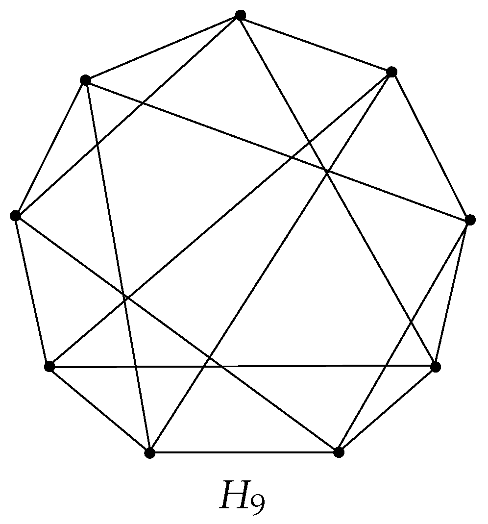
Example 1.

Let $H_n$ be an $\left(\frac{n-1}{2}\right)$-regular graph with $diam\left(H_n\right)=diam\left(\overline{H_n}\right)=2$, where n is odd. The graph $H_9$ has been shown in Figure 1. We have $DD\left(H_9\right)+DD\left(\overline{H_9}\right)=864=6min\left\{\delta ,n-1-\Delta \right\}\left(\genfrac{}{}{0pt}{}{n}{2}\right)$.

Proposition 1.

Let $\Gamma \in {\mathcal{G}}_n$ with m edges and maximum degree Δ, minimum degree δ. Then

$\left(1\right)$

$$\begin{array}{cc}& 6min\left\{\delta ,n-1-\Delta \right\}\left(\genfrac{}{}{0pt}{}{n}{2}\right)\le DD(\Gamma )+DD\left(\overline{\Gamma }\right)\\ & \le \frac{1}{3}(n^3+3n^2+2n-6)max\left\{\Delta ,n-1-\delta \right\}.\end{array}$$

(1)

The left equality holds in (1) if and only if Γ is an $\left(\frac{n-1}{2}\right)$-regular graph with $diam(\Gamma )=diam\left(\overline{\Gamma }\right)=2$, where n is odd.

$\left(2\right)$

$$\begin{array}{ccc}& & 4\delta (n-1-\Delta )\left[2{\left(\genfrac{}{}{0pt}{}{n}{2}\right)}^2+\left(\genfrac{}{}{0pt}{}{n}{2}\right)(n-1)-{(n-1)}^2\right]<DD(\Gamma )·DD\left(\overline{\Gamma }\right)\hfill \\ & & <4{\left(\genfrac{}{}{0pt}{}{n}{2}\right)}^2\Delta (n-1-\delta )max\left\{2n-2,9\right\}.\hfill \end{array}$$

(2)

Proof. 

$\left(1\right)$ From the definition of degree distance with Lemma 1, we obtain

$$\begin{array}{ccc}\hfill DD(\Gamma )+DD\left(\overline{\Gamma }\right)& \le & 2\Delta W(\Gamma )+2\overline{\Delta }W\left(\overline{\Gamma }\right)\hfill \\ & =& 2\Delta W(\Gamma )+2(n-1-\delta )W\left(\overline{\Gamma }\right)\hfill \\ & \le & 2max\left\{\Delta ,n-1-\delta \right\}\left(W(\Gamma )+W\left(\overline{\Gamma }\right)\right)\hfill \\ & \le & \frac{1}{3}(n^3+3n^2+2n-6)max\left\{\Delta ,n-1-\delta \right\}\hfill \end{array}$$

and

$$\begin{array}{ccc}\hfill DD(\Gamma )+DD\left(\overline{\Gamma }\right)& \ge & 2\delta W(\Gamma )+2\overline{\delta }W\left(\overline{\Gamma }\right)\hfill \\ & =& 2\delta W(\Gamma )+2(n-1-\Delta )W\left(\overline{\Gamma }\right)\hfill \\ & \ge & 2min\left\{\delta ,n-1-\Delta \right\}\left(W(\Gamma )+W\left(\overline{\Gamma }\right)\right)\hfill \\ & \ge & 6min\left\{\delta ,n-1-\Delta \right\}\left(\genfrac{}{}{0pt}{}{n}{2}\right).\hfill \end{array}$$

From the above, the left equality holds in (1) if and only if $de{g}_{\Gamma }\left(u\right)+de{g}_{\Gamma }\left(v\right)=2\delta$ for any $u,v\in V(\Gamma )$, $\delta =n-1-\Delta$ and $diam(\Gamma )=diam\left(\overline{\Gamma }\right)=2$, by Remark 1. Hence, the left equality holds in (1) if and only if $\Gamma$ is an $\left(\frac{n-1}{2}\right)$-regular graph with $diam(\Gamma )=diam\left(\overline{\Gamma }\right)=2$, where n is odd.

$\left(2\right)$ From Lemma 2, we obtain $diam\left(G\right)·diam\left(\overline{G}\right)\le max\{2(n-1),9\}$. Since $\Gamma \in {\mathcal{G}}_n$, both $\Gamma$ and $\overline{\Gamma }$ are connected and hence $diam(\Gamma )\ge 2\le diam\left(\overline{\Gamma }\right)$. Using this result with the definition of Wiener index, we obtain

$$W(\Gamma )·W\left(\overline{\Gamma }\right)<diam\left(G\right)·diam\left(\overline{G}\right){\left(\genfrac{}{}{0pt}{}{n}{2}\right)}^2\le max\{2(n-1),9\}{\left(\genfrac{}{}{0pt}{}{n}{2}\right)}^2.$$

Using the above result with the definition of degree distance, we obtain

$$\begin{array}{ccc}\hfill DD(\Gamma )·DD\left(\overline{\Gamma }\right)& \le & 2\Delta W(\Gamma )·2\overline{\Delta }W\left(\overline{\Gamma }\right)\hfill \\ & =& 4\Delta (n-1-\delta )W(\Gamma )·W\left(\overline{\Gamma }\right)\hfill \\ & <& 4{\left(\genfrac{}{}{0pt}{}{n}{2}\right)}^2\Delta (n-1-\delta )max\{2n-2,9\}.\hfill \end{array}$$

Since both $\Gamma$ and $\overline{\Gamma }$ are connected, we have $n-1\le m,\overline{m}\le \left[\left(\genfrac{}{}{0pt}{}{n}{2}\right)-(n-1)\right](n-1)$ with $n>3$. Moreover, we have $m+\overline{m}=\left(\genfrac{}{}{0pt}{}{n}{2}\right)$. Let us consider a function

$$f\left(x\right)=x\left[\left(\genfrac{}{}{0pt}{}{n}{2}\right)-x\right],n-1\le x\le \left(\genfrac{}{}{0pt}{}{n}{2}\right)-(n-1).$$

Then one can easily see that $f\left(x\right)$ is an increasing function on $n-1\le x\le \frac{1}{2}\left(\genfrac{}{}{0pt}{}{n}{2}\right)$ and a decreasing function on $\frac{1}{2}\left(\genfrac{}{}{0pt}{}{n}{2}\right)\le x\le \left(\genfrac{}{}{0pt}{}{n}{2}\right)-(n-1)$. Hence

$$f\left(x\right)=x\left[\left(\genfrac{}{}{0pt}{}{n}{2}\right)-x\right]\ge \left[\left(\genfrac{}{}{0pt}{}{n}{2}\right)-(n-1)\right](n-1)$$

with equality if and only if $x=n-1$. Now, we must prove that

$$W(\Gamma )·W\left(\overline{\Gamma }\right)\ge 2{\left(\genfrac{}{}{0pt}{}{n}{2}\right)}^2+\left[\left(\genfrac{}{}{0pt}{}{n}{2}\right)-(n-1)\right](n-1)$$

(3)

with equality if and only if $diam(\Gamma )=diam\left(\overline{\Gamma }\right)=2$ and $m=n-1$.

From the above with the definition of the Wiener index, we obtain

$$\begin{array}{cc}\hfill W(\Gamma )·W\left(\overline{\Gamma }\right)& \ge \left[m+\left(\left(\genfrac{}{}{0pt}{}{n}{2}\right)-m\right)2\right]\left[\overline{m}+\left(\left(\genfrac{}{}{0pt}{}{n}{2}\right)-\overline{m}\right)2\right]\hfill \\ \hfill & =\left[2\left(\genfrac{}{}{0pt}{}{n}{2}\right)-m\right]\left[2\left(\genfrac{}{}{0pt}{}{n}{2}\right)-\overline{m}\right]\hfill \\ \hfill & =2{\left(\genfrac{}{}{0pt}{}{n}{2}\right)}^2+m\left[\left(\genfrac{}{}{0pt}{}{n}{2}\right)-m\right]\hfill \\ \hfill & \ge 2{\left(\genfrac{}{}{0pt}{}{n}{2}\right)}^2+\left[\left(\genfrac{}{}{0pt}{}{n}{2}\right)-(n-1)\right](n-1).\hfill \end{array}$$

Moreover, the equality holds in (3) if and only if the above two equalities hold, i.e., if and only if $diam(\Gamma )=diam\left(\overline{\Gamma }\right)=2$ and $m=n-1$. Now,

$$\begin{array}{ccc}\hfill DD(\Gamma )·DD\left(\overline{\Gamma }\right)& \ge & 2\delta W(\Gamma )·2\overline{\delta }W\left(\overline{\Gamma }\right)\hfill \\ & =& 4\delta (n-1-\Delta )W(\Gamma )·W\left(\overline{\Gamma }\right)\hfill \\ & \ge & 4\delta (n-1-\Delta )\left[2{\left(\genfrac{}{}{0pt}{}{n}{2}\right)}^2+\left(\genfrac{}{}{0pt}{}{n}{2}\right)(n-1)-{(n-1)}^2\right].\hfill \end{array}$$

(4)

The equality holds in (4) if and only if $\Gamma$ is a regular graph. Hence the left inequality in (2) is strict as any regular graph $\Gamma \in {\mathcal{G}}_n$ has more than $n-1$ edges. □

3. Nordhaus–Gaddum-Type Results for Steiner Wiener $\mathit{k}$-Index

Mao et al. [38] obtained the Nordhaus–Gaddum-type results for Steiner Wiener index.

Lemma 3

([38]). Let $\Gamma \in \mathcal{G}\left(n\right)$ and let k be an integer with $3\le k\le n$. Then

$$\begin{array}{cc}\hfill \left(1\right)& \left(\genfrac{}{}{0pt}{}{n}{k}\right)(2k-2)\le {SW}_k(\Gamma )+{SW}_k\left(\overline{\Gamma }\right)\le max\left\{n+k-1,4k-2\right\}\left(\genfrac{}{}{0pt}{}{n}{k}\right),\hfill \\ \hfill \left(2\right)& {(k-1)}^2{\left(\genfrac{}{}{0pt}{}{n}{k}\right)}^2\le {SW}_k(\Gamma )·{SW}_k\left(\overline{\Gamma }\right)\le max\left\{k(n-1),{(2k-1)}^2\right\}{\left(\genfrac{}{}{0pt}{}{n}{k}\right)}^2.\hfill \end{array}$$

Moreover, the lower bounds are sharp.

We now obtain some upper bound on $d_{\Gamma }\left(S\right)+d_{\overline{\Gamma }}\left(S\right)$ and $d_{\Gamma }\left(S\right)·d_{\overline{\Gamma }}\left(S\right)$.

Lemma 4

Let $\Gamma \in {\mathcal{G}}_n$ and also let $S\subseteq V(\Gamma )$ and $\left|S\right|=k$ with $2\le k\le n$. Then:

$$\begin{array}{cc}\hfill \left(1\right)& d_{\Gamma }\left(S\right)+d_{\overline{\Gamma }}\left(S\right)\le n+k-2,\hfill \\ \hfill \left(2\right)& d_{\Gamma }\left(S\right)·d_{\overline{\Gamma }}\left(S\right)\le (n-1)(k-1).\hfill \end{array}$$

Proof. 

Since $S\subseteq V(\Gamma )$ and $\left|S\right|=k$, we now consider induced subgraphs $\Gamma \left[S\right]$ and $\overline{\Gamma }\left[S\right]$. From the definition of Steiner distance, we obtain

$$k-1\le d_{\Gamma }\left(S\right),d_{\overline{\Gamma }}\left(S\right)\le n-1.$$

If $\Gamma \left[S\right]$ is connected, then $d_{\Gamma }\left(S\right)=k-1$ and hence $d_{\Gamma }\left(S\right)+d_{\overline{\Gamma }}\left(S\right)\le n+k-2$, $d_{\Gamma }\left(S\right)·d_{\overline{\Gamma }}\left(S\right)\le (n-1)(k-1)$. Otherwise, $\Gamma \left[S\right]$ is disconnected, i.e., $\overline{\Gamma }\left[S\right]$ is connected. Thus, we have $d_{\overline{\Gamma }}\left(S\right)=k-1$ and hence $d_{\Gamma }\left(S\right)+d_{\overline{\Gamma }}\left(S\right)\le n+k-2$, $d_{\Gamma }\left(S\right)·d_{\overline{\Gamma }}\left(S\right)\le (n-1)(k-1)$. This completes the proof. □

Theorem 1.

Let $\Gamma \in {\mathcal{G}}_n$ and also let k be an integer with $2\le k\le n$. Then:

$$\begin{array}{cc}\hfill \left(1\right)& {SW}_k(\Gamma )+{SW}_k\left(\overline{\Gamma }\right)\le (n+k-2)\left(\genfrac{}{}{0pt}{}{n}{k}\right),\hfill \\ \hfill \left(2\right)& {SW}_k(\Gamma )·{SW}_k\left(\overline{\Gamma }\right)\le \frac{1}{4}{(n+k-2)}^2{\left(\genfrac{}{}{0pt}{}{n}{k}\right)}^2.\hfill \end{array}$$

Proof. 

For $S\subseteq V(\Gamma )$ and $\left|S\right|=k$, from the definition of Steiner Wiener k-index or k-center Steiner Wiener index${SW}_k(\Gamma )$ of graph $\Gamma$ with Lemma 4, we obtain

$$\begin{array}{cc}\hfill {SW}_k(\Gamma )+{SW}_k\left(\overline{\Gamma }\right)& =\sum _{\genfrac{}{}{0pt}{}{S\subseteq V(\Gamma )}{\left|S\right|=k}}{d}_{\Gamma }\left(S\right)+\sum _{\genfrac{}{}{0pt}{}{S\subseteq V\left(\overline{\Gamma }\right)}{\left|S\right|=k}}{d}_{\overline{\Gamma }}\left(S\right)\hfill \\ \hfill & =\sum _{\genfrac{}{}{0pt}{}{S\subseteq V(\Gamma )}{\left|S\right|=k}}\left(d_{\Gamma }\left(S\right)+d_{\overline{\Gamma }}\left(S\right)\right)\hfill \\ \hfill & \le (n+k-2)\left(\genfrac{}{}{0pt}{}{n}{k}\right)\hfill \end{array}$$

and

$$\begin{array}{cc}\hfill {SW}_k(\Gamma )·{SW}_k\left(\overline{\Gamma }\right)& =\sum _{\genfrac{}{}{0pt}{}{S\subseteq V(\Gamma )}{\left|S\right|=k}}{d}_{\Gamma }\left(S\right)·\sum _{\genfrac{}{}{0pt}{}{S\subseteq V\left(\overline{\Gamma }\right)}{\left|S\right|=k}}{d}_{\overline{\Gamma }}\left(S\right)\hfill \\ \hfill & \le \frac{1}{4}{\left[\sum _{\genfrac{}{}{0pt}{}{S\subseteq V(\Gamma )}{\left|S\right|=k}}\left(d_{\Gamma }\left(S\right)+d_{\overline{\Gamma }}\left(S\right)\right)\right]}^2\hfill \\ \hfill & \le \frac{1}{4}{(n+k-2)}^2{\left(\genfrac{}{}{0pt}{}{n}{k}\right)}^2.\hfill \end{array}$$

This completes the proof. □

Remark 3.

If $k\ge \frac{n}{3}$, then the upper bound in Theorem 1$\left(1\right)$ is always better than the upper bound in Lemma 3$\left(1\right)$ because

$$max\left\{n+k-1,4k-2\right\}\ge n+k-2.$$

Moreover, the upper bound in Theorem 1 $\left(1\right)$ is more simple than the upper bound in Lemma 3$\left(1\right)$.

Remark 4.

If $k\ge n-2\sqrt{n-1}$, then the upper bound in Theorem 1$\left(2\right)$ is always better than the upper bound in Lemma 3$\left(2\right)$.

We must prove that

$$\frac{1}{4}{(n+k-2)}^2\le k(n-1),$$

that is,

$${(n+k-2)}^2\le 4(k-1)(n-1)+4(n-1),$$

that is,

$${(n-k)}^2\le 4(n-1),$$

that is,

$$k\ge n-2\sqrt{n-1},$$

which is true always. Moreover, we must prove that

$$\frac{1}{4}{(n+k-2)}^2\le {(2k-1)}^2,$$

that is,

$$n+k-2\le 2(2k-1),$$

that is,

$$k\ge \frac{n}{3},$$

which is true always as $k\ge n-2\sqrt{n-1}\ge \frac{n}{3}$. Hence the result.

4. Nordhaus–Gaddum-Type Results for $\mathit{k}$-Center Steiner Degree Distance ${SDD}_{\mathit{k}}(\Gamma )$

Mao et al. [46] derived sharp upper and lower bounds of ${SDD}_k(\Gamma )$ in terms of order and size.

Lemma 5

([46]). Let $\Gamma \in \mathcal{G}(n,m)$, and let k be an integer with $2\le k\le n$. Then

$$2m\left(\genfrac{}{}{0pt}{}{n-1}{k-1}\right)(k-1)\le {SDD}_k(\Gamma )\le 2m\left(\genfrac{}{}{0pt}{}{n-1}{k-1}\right)(n-1)$$

Moreover, the upper and lower bounds are sharp.

For $\Gamma \in \mathcal{G}(n,m)$, we have the following by above lemma.

Theorem 2.

Let $\Gamma \in \mathcal{G}(n,m)$ and let k be an integer with $2\le k\le n$. Then

$$2(k-1)\left(\genfrac{}{}{0pt}{}{n-1}{k-1}\right)\left(\genfrac{}{}{0pt}{}{n}{2}\right)\le {SDD}_k(\Gamma )+{SDD}_k\left(\overline{\Gamma }\right)\le 2(n-1)\left(\genfrac{}{}{0pt}{}{n-1}{k-1}\right)\left(\genfrac{}{}{0pt}{}{n}{2}\right)$$

and

$$4m{(k-1)}^2{\left(\genfrac{}{}{0pt}{}{n-1}{k-1}\right)}^2\left[\left(\genfrac{}{}{0pt}{}{n}{2}\right)-m\right]\le {SDD}_k(\Gamma )·{SDD}_k\left(\overline{\Gamma }\right)\le 4m{(n-1)}^2{\left(\genfrac{}{}{0pt}{}{n-1}{k-1}\right)}^2\left[\left(\genfrac{}{}{0pt}{}{n}{2}\right)-m\right].$$

Moreover, the upper and lower bounds are sharp.

Proof. 

From Lemma 5, we have

$$2m\left(\genfrac{}{}{0pt}{}{n-1}{k-1}\right)(k-1)\le {SDD}_k(\Gamma )\le 2m\left(\genfrac{}{}{0pt}{}{n-1}{k-1}\right)(n-1).$$

and

$$2(k-1)\left(\genfrac{}{}{0pt}{}{n-1}{k-1}\right)\left[\left(\genfrac{}{}{0pt}{}{n}{2}\right)-m\right]\le {SDD}_k\left(\overline{\Gamma }\right)\le 2(n-1)\left(\genfrac{}{}{0pt}{}{n-1}{k-1}\right)\left[\left(\genfrac{}{}{0pt}{}{n}{2}\right)-m\right].$$

Therefore, we have

$$2(k-1)\left(\genfrac{}{}{0pt}{}{n-1}{k-1}\right)\left(\genfrac{}{}{0pt}{}{n}{2}\right)\le {SDD}_k(\Gamma )+{SDD}_k\left(\overline{\Gamma }\right)\le 2(n-1)\left(\genfrac{}{}{0pt}{}{n-1}{k-1}\right)\left(\genfrac{}{}{0pt}{}{n}{2}\right)$$

and

$$4m{(k-1)}^2{\left(\genfrac{}{}{0pt}{}{n-1}{k-1}\right)}^2\left[\left(\genfrac{}{}{0pt}{}{n}{2}\right)-m\right]\le {SDD}_k(\Gamma )·{SDD}_k\left(\overline{\Gamma }\right)\le 4m{(n-1)}^2{\left(\genfrac{}{}{0pt}{}{n-1}{k-1}\right)}^2\left[\left(\genfrac{}{}{0pt}{}{n}{2}\right)-m\right].$$

It is clear that the bounds are sharp when $k=n$. □

Let ${\Omega }_1$ be a class of graphs $\Gamma =(V,E)$ such that $d_{\Gamma }\left(S\right)=k-1$ for any $S\subseteq V(\Gamma )$ with $v_1\in S$, $\left|S\right|=k$, and $de{g}_{\Gamma }\left(v_1\right)=\Delta >\delta =de{g}_{\Gamma }\left(v_2\right)=de{g}_{\Gamma }\left(v_3\right)=\cdots =de{g}_{\Gamma }\left(v_n\right)$, where $\Gamma$ has the maximum degree $\Delta$ and all the remaining $n-1$ vertices of degree $\delta$. If $\Gamma \in {\Omega }_1$, then $\Delta (\Gamma )\ge n-k+1$. Let ${\Omega }_2$ be a class of graphs $\Gamma =(V,E)$ such that $d_{\Gamma }\left(S\right)=k-1$ for any $S\subseteq V(\Gamma )$ with $v_n\in S$, $\left|S\right|=k$, and $de{g}_{\Gamma }\left(v_n\right)=\delta <\Delta =de{g}_{\Gamma }\left(v_{n-1}\right)=de{g}_{\Gamma }\left(v_{n-2}\right)=\cdots =de{g}_{\Gamma }\left(v_1\right)$, where $\Gamma$ has the minimum degree $\delta$ and all the remaining $n-1$ vertices of degree $\Delta$. If $\Gamma \in {\Omega }_2$, then $\delta (\Gamma )\ge n-k+1$. We now give upper and lower bounds on ${SDD}_k(\Gamma )$.

Theorem 3.

Let Γ be a connected graph of order n, and let k be an integer with $2\le k\le n$. Then

$$\left(\genfrac{}{}{0pt}{}{n-1}{k-1}\right)(k-1)(\Delta -\delta )+k\delta {SW}_k(\Gamma )\le {SDD}_k(\Gamma )\le k\Delta {SW}_k(\Gamma )-\left(\genfrac{}{}{0pt}{}{n-1}{k-1}\right)(k-1)(\Delta -\delta ),$$

(5)

where Δ and δ are the maximum and the minimum degree of graph Γ, respectively. Moreover, the left (right) equality holds if and only if Γ is a regular graph or $\Gamma \in {\Omega }_1$$(\Gamma \in {\Omega }_2)$.

Proof. 

Let ${\rm Y}=\left\{S\subseteq V(\Gamma ):\left|S\right|=k\right\}$. Then $|{\rm Y}|=\left(\genfrac{}{}{0pt}{}{n}{k}\right)$.

Lower Bound: Let $v_1$ be the maximum degree vertex in $\Gamma$. Then $de{g}_{\Gamma }\left(v_1\right)=\Delta$. Denote by

$${{\rm Y}}_1=\left\{S\subseteq V(\Gamma ):\left|S\right|=k \mathrm{and} v_1\in S\right\}\mathrm{and}{{\rm Y}}_2=\left\{S\subseteq V(\Gamma )\backslash \left\{v_1\right\}:\left|S\right|=k\right\}.$$

Then ${\rm Y}={{\rm Y}}_1\cup {{\rm Y}}_2$ and $|{\rm Y}|=|{{\rm Y}}_1|+|{{\rm Y}}_2|$ as ${{\rm Y}}_1\cap {{\rm Y}}_2=\varnothing$. Moreover,

$$|{{\rm Y}}_1|=\left(\genfrac{}{}{0pt}{}{n-1}{k-1}\right)\mathrm{and}\left|{{\rm Y}}_2\right|=\left(\genfrac{}{}{0pt}{}{n-1}{k}\right).$$

One can easily see that

$$\sum _{v\in S}de{g}_{\Gamma }\left(v\right)\ge \left\{\begin{array}{cc}\Delta +(k-1)\delta \hfill & \mathrm{for}\mathrm{any}S\in {{\rm Y}}_1,\hfill \\ k\delta \hfill & \mathrm{for}\mathrm{any}S\in {{\rm Y}}_2.\hfill \end{array}\right.$$

We obtain

$$\begin{array}{cc}\hfill {SDD}_k(\Gamma )& =\sum _{\stackrel{S\subseteq V(\Gamma )}{\left|S\right|=k}}\left[\sum _{v\in S}de{g}_{\Gamma }\left(v\right)\right]d_{\Gamma }\left(S\right)\hfill \\ \hfill & =\sum _{S\in {{\rm Y}}_1}\left[\sum _{v\in S}de{g}_{\Gamma }\left(v\right)\right]d_{\Gamma }\left(S\right)+\sum _{S\in {{\rm Y}}_2}\left[\sum _{v\in S}de{g}_{\Gamma }\left(v\right)\right]d_{\Gamma }\left(S\right)\hfill \\ \hfill & \ge \sum _{S\in {{\rm Y}}_1}\left(\Delta +(k-1)\delta \right)d_{\Gamma }\left(S\right)+k\delta \sum _{S\in {{\rm Y}}_2}{d}_{\Gamma }\left(S\right)\hfill \\ \hfill & =(\Delta -\delta )\sum _{S\in {{\rm Y}}_1}{d}_{\Gamma }\left(S\right)+k\delta \left[\sum _{S\in {{\rm Y}}_1}{d}_{\Gamma }\left(S\right)+\sum _{S\in {{\rm Y}}_2}{d}_{\Gamma }\left(S\right)\right]\hfill \\ \hfill \end{array}$$

(6)

$$\begin{array}{cc}\hfill & \ge (\Delta -\delta )(k-1)|{{\rm Y}}_1|+k\delta \sum _{S\in {\rm Y}}{d}_{\Gamma }\left(S\right)\hfill \\ \hfill & =\left(\genfrac{}{}{0pt}{}{n-1}{k-1}\right)(k-1)(\Delta -\delta )+k\delta {SW}_k(\Gamma ).\hfill \end{array}$$

(7)

The first part of the proof is complete.

Moreover, the equality holds in (6) if and only if $de{g}_{\Gamma }\left(v\right)=\delta$ for all $v\in V(\Gamma )\backslash \left\{v_1\right\}$. The equality holds in (7) if and only if $d_{\Gamma }\left(S\right)=k-1$ for $S\in {{\rm Y}}_1$. From these two results, we conclude that the left equality holds in (5) if and only if $\Gamma$ is a regular graph or $\Gamma \in {\Omega }_1$.

Upper Bound: Let $v_n$ be the minimum degree vertex in $\Gamma$. Then $de{g}_{\Gamma }\left(v_n\right)=\delta$. Denote by

$${{\rm Y}}_1^{\prime }=\left\{S\subseteq V(\Gamma ):\left|S\right|=k \mathrm{and} v_n\in S\right\}\mathrm{and}{{\rm Y}}_2^{\prime }=\left\{S\subseteq V(\Gamma )\backslash \left\{v_n\right\}:\left|S\right|=k\right\}.$$

Then ${\rm Y}={{\rm Y}}_1^{\prime }\cup {{\rm Y}}_2^{\prime }$ and $|{\rm Y}|=|{{\rm Y}}_1^{\prime }|+|{{\rm Y}}_2^{\prime }|$ as ${{\rm Y}}_1^{\prime }\cap {{\rm Y}}_2^{\prime }=\varnothing$. Moreover,

$$|{{\rm Y}}_1^{\prime }|=\left(\genfrac{}{}{0pt}{}{n-1}{k-1}\right)\mathrm{and}\left|{{\rm Y}}_2^{\prime }\right|=\left(\genfrac{}{}{0pt}{}{n-1}{k}\right).$$

One can easily see that

$$\sum _{v\in S}de{g}_{\Gamma }\left(v\right)\le \left\{\begin{array}{cc}\delta +(k-1)\Delta \hfill & \mathrm{for}\mathrm{any}S\in {{\rm Y}}_1^{\prime },\hfill \\ k\Delta \hfill & \mathrm{for}\mathrm{any}S\in {{\rm Y}}_2^{\prime }.\hfill \end{array}\right.$$

Similarly, we obtain

$$\begin{array}{cc}\hfill {SDD}_k(\Gamma )& =\sum _{S\in {{\rm Y}}_1^{\prime }}\left[\sum _{v\in S}de{g}_{\Gamma }\left(v\right)\right]d_{\Gamma }\left(S\right)+\sum _{S\in {{\rm Y}}_2^{\prime }}\left[\sum _{v\in S}de{g}_{\Gamma }\left(v\right)\right]d_{\Gamma }\left(S\right)\hfill \end{array}$$

$$\begin{array}{cc}\hfill & \hspace{1em}\hspace{1em}\hspace{1em}\hspace{1em}\le \sum _{S\in {{\rm Y}}_1^{\prime }}\left(\delta +(k-1)\Delta \right)d_{\Gamma }\left(S\right)+k\Delta \sum _{S\in {{\rm Y}}_2^{\prime }}{d}_{\Gamma }\left(S\right)\hfill \\ \hfill & \hspace{1em}\hspace{1em}\hspace{1em}\hspace{1em}=k\Delta \left[\sum _{S\in {{\rm Y}}_1^{\prime }}{d}_{\Gamma }\left(S\right)+\sum _{S\in {{\rm Y}}_2^{\prime }}{d}_{\Gamma }\left(S\right)\right]-(\Delta -\delta )\sum _{S\in {{\rm Y}}_1^{\prime }}{d}_{\Gamma }\left(S\right)\hfill \end{array}$$

(8)

$$\begin{array}{cc}\hfill & \le k\Delta \sum _{S\in {\rm Y}}{d}_{\Gamma }\left(S\right)-(\Delta -\delta )(k-1)\left|{{\rm Y}}_1^{\prime }\right|\hfill \\ \hfill & =k\Delta {SW}_k(\Gamma )-\left(\genfrac{}{}{0pt}{}{n-1}{k-1}\right)(k-1)(\Delta -\delta ).\hfill \end{array}$$

(9)

Moreover, the equality holds in (8) if and only if $de{g}_{\Gamma }\left(v\right)=\Delta$ for all $v\in V(\Gamma )\backslash \left\{v_n\right\}$. The equality holds in (9) if and only if $d_{\Gamma }\left(S\right)=k-1$ for $S\in {{\rm Y}}_1^{\prime }$. From these two results, we conclude that the right equality holds in (5) if and only if $\Gamma$ is a regular graph or $\Gamma \in {\Omega }_2$. □

Corollary 1

([46]). Let Γ be a connected graph of order n, and let k be an integer with $2\le k\le n$. Then

$$k\delta {SW}_k(\Gamma )\le {SDD}_k(\Gamma )\le k\Delta {SW}_k(\Gamma )$$

with equality if and only if Γ is a regular graph.

We now give a sharp upper and lower bounds of ${SDD}_k(\Gamma )+{SDD}_k\left(\overline{\Gamma }\right)$ and ${SDD}_k(\Gamma )·{SDD}_k\left(\overline{\Gamma }\right)$ in terms of order, maximum degree and minimum degree.

Theorem 4.

Let $\Gamma \in {\mathcal{G}}_n$ and let k be an integer with $2\le k\le n$. Then

$\left(1\right)$

$$\begin{array}{ccc}& & \left(\genfrac{}{}{0pt}{}{n}{k}\right)2k(k-1)\left[min\left\{\delta ,n-1-\Delta \right\}+\frac{1}{n}(\Delta -\delta )\right]\hfill \\ & \le & {SDD}_k(\Gamma )+{SDD}_k\left(\overline{\Gamma }\right)\le \left(\genfrac{}{}{0pt}{}{n}{k}\right)k\left[(n+k-2)max\left\{\Delta ,n-1-\delta \right\}-\frac{2(k-1)}{n}(\Delta -\delta )\right].\hfill \end{array}$$

$\left(2\right)$

$$\begin{array}{cc}\hfill & k^2\delta (n-1-\Delta ){(k-1)}^2{\left(\genfrac{}{}{0pt}{}{n}{k}\right)}^2+{\left(\genfrac{}{}{0pt}{}{n-1}{k-1}\right)}^2{(k-1)}^2{(\Delta -\delta )}^2\hfill \\ \hfill & +{\left(\genfrac{}{}{0pt}{}{n}{k}\right)}^2\frac{2k^2{(k-1)}^2}{n}(\Delta -\delta )min\left\{\delta ,n-1-\Delta \right\}\le {SDD}_k(\Gamma )·{SDD}_k\left(\overline{\Gamma }\right)\hfill \\ \hfill & \le \frac{1}{4}{\left(\genfrac{}{}{0pt}{}{n}{k}\right)}^2{(n+k-2)}^2{k}^2\Delta (n-1-\delta )+{\left(\genfrac{}{}{0pt}{}{n-1}{k-1}\right)}^2{(k-1)}^2{(\Delta -\delta )}^2\hfill \\ \hfill & -\left(\genfrac{}{}{0pt}{}{n-1}{k-1}\right)k(k-1)(\Delta -\delta )\left(\genfrac{}{}{0pt}{}{n}{k}\right)(n+k-2)max\left\{\Delta ,n-1-\delta \right\}.\hfill \end{array}$$

Proof. 

$\left(1\right)$ Using Theorems 1 and 3, we obtain

$$\begin{array}{ccc}& & {SDD}_k(\Gamma )+{SDD}_k\left(\overline{\Gamma }\right)\hfill \\ & & \le k\Delta {SW}_k(\Gamma )-\left(\genfrac{}{}{0pt}{}{n-1}{k-1}\right)(k-1)(\Delta -\delta )+k\overline{\Delta }{SW}_k\left(\overline{\Gamma }\right)-\left(\genfrac{}{}{0pt}{}{n-1}{k-1}\right)(k-1)(\overline{\Delta }-\overline{\delta })\hfill \\ & & =k\left[\Delta {SW}_k(\Gamma )+k(n-1-\delta ){SW}_k\left(\overline{\Gamma }\right)\right]-2\left(\genfrac{}{}{0pt}{}{n-1}{k-1}\right)(k-1)(\Delta -\delta )\hfill \\ & & \le kmax\left\{\Delta ,n-1-\delta \right\}\left[{SW}_k(\Gamma )+{SW}_k\left(\overline{\Gamma }\right)\right]-2\left(\genfrac{}{}{0pt}{}{n}{k}\right)\frac{k}{n}(k-1)(\Delta -\delta )\hfill \\ & & \le \left(\genfrac{}{}{0pt}{}{n}{k}\right)k\left[(n+k-2)max\left\{\Delta ,n-1-\delta \right\}-\frac{2(k-1)}{n}(\Delta -\delta )\right].\hfill \end{array}$$

and

$$\begin{array}{ccc}& & {SDD}_k(\Gamma )+{SDD}_k\left(\overline{\Gamma }\right)\hfill \\ & & \ge k\delta {SW}_k(\Gamma )+\left(\genfrac{}{}{0pt}{}{n-1}{k-1}\right)(k-1)(\Delta -\delta )+k\overline{\delta }{SW}_k\left(\overline{\Gamma }\right)+\left(\genfrac{}{}{0pt}{}{n-1}{k-1}\right)(k-1)(\overline{\Delta }-\overline{\delta })\hfill \\ & & =k\left[\delta {SW}_k(\Gamma )+(n-1-\Delta ){SW}_k\left(\overline{\Gamma }\right)\right]+2\left(\genfrac{}{}{0pt}{}{n-1}{k-1}\right)(k-1)(\Delta -\delta )\hfill \\ & & \ge kmin\left\{\delta ,n-1-\Delta \right\}\left[{SW}_k(\Gamma )+{SW}_k\left(\overline{\Gamma }\right)\right]+2\left(\genfrac{}{}{0pt}{}{n}{k}\right)\frac{k}{n}(k-1)(\Delta -\delta )\hfill \\ & & \ge \left(\genfrac{}{}{0pt}{}{n}{k}\right)2k(k-1)\left[min\left\{\delta ,n-1-\Delta \right\}+\frac{1}{n}(\Delta -\delta )\right].\hfill \end{array}$$

$\left(2\right)$ Using Theorems 1 and 3, we obtain

$$\begin{array}{ccc}& & {SDD}_k(\Gamma )·{SDD}_k\left(\overline{\Gamma }\right)\hfill \\ & & \le \left[k\Delta {SW}_k(\Gamma )-\left(\genfrac{}{}{0pt}{}{n-1}{k-1}\right)(k-1)(\Delta -\delta )\right]·\left[k\overline{\Delta }{SW}_k\left(\overline{\Gamma }\right)-\left(\genfrac{}{}{0pt}{}{n-1}{k-1}\right)(k-1)(\overline{\Delta }-\overline{\delta })\right]\hfill \\ & & =k^2\Delta (n-1-\delta (\Gamma )){SW}_k(\Gamma )·{SW}_k\left(\overline{\Gamma }\right)+{\left(\genfrac{}{}{0pt}{}{n-1}{k-1}\right)}^2{(k-1)}^2{(\Delta -\delta )}^2\hfill \\ & & -\left(\genfrac{}{}{0pt}{}{n-1}{k-1}\right)k(k-1)(\Delta -\delta )\left[\Delta {SW}_k(\Gamma )+(n-1-\delta ){SW}_k\left(\overline{\Gamma }\right)\right]\hfill \\ & & \le \frac{1}{4}{\left(\genfrac{}{}{0pt}{}{n}{k}\right)}^2{(n+k-2)}^2{k}^2\Delta (n-1-\delta )+{\left(\genfrac{}{}{0pt}{}{n-1}{k-1}\right)}^2{(k-1)}^2{(\Delta -\delta )}^2\hfill \\ & & -\left(\genfrac{}{}{0pt}{}{n-1}{k-1}\right)k(k-1)\left(\Delta -\delta \right)\left(\genfrac{}{}{0pt}{}{n}{k}\right)(n+k-2)max\left\{\Delta ,n-1-\delta \right\}.\hfill \end{array}$$

and

$$\begin{array}{ccc}& & {SDD}_k(\Gamma )·{SDD}_k\left(\overline{\Gamma }\right)\hfill \\ & & \ge \left[k\delta {SW}_k(\Gamma )+\left(\genfrac{}{}{0pt}{}{n-1}{k-1}\right)(k-1)(\Delta -\delta )\right]·\left[k\overline{\delta }{SW}_k\left(\overline{\Gamma }\right)+\left(\genfrac{}{}{0pt}{}{n-1}{k-1}\right)(k-1)(\overline{\Delta }-\overline{\delta })\right]\hfill \\ & & =k^2\delta (n-1-\Delta ){SW}_k(\Gamma )·{SW}_k\left(\overline{\Gamma }\right)+{\left(\genfrac{}{}{0pt}{}{n-1}{k-1}\right)}^2{(k-1)}^2{(\Delta -\delta )}^2\hfill \\ & & +\left(\genfrac{}{}{0pt}{}{n-1}{k-1}\right)k(k-1)(\Delta -\delta )\left[\delta {SW}_k(\Gamma )+(n-1-\Delta ){SW}_k\left(\overline{\Gamma }\right)\right]\hfill \\ & & \ge k^2\delta (n-1-\Delta ){(k-1)}^2{\left(\genfrac{}{}{0pt}{}{n}{k}\right)}^2+{\left(\genfrac{}{}{0pt}{}{n-1}{k-1}\right)}^2{(k-1)}^2{(\Delta -\delta )}^2\hfill \\ & & +{\left(\genfrac{}{}{0pt}{}{n}{k}\right)}^2\frac{2k^2{(k-1)}^2}{n}(\Delta -\delta )min\left\{\delta ,n-1-\Delta \right\}\hfill \end{array}$$

as

$$\begin{array}{cc}\hfill \delta {SW}_k(\Gamma )+(n-1-\Delta ){SW}_k\left(\overline{\Gamma }\right)& \ge min\left\{\delta ,n-1-\Delta \right\}\left[{SW}_k(\Gamma )+{SW}_k\left(\overline{\Gamma }\right)\right]\hfill \\ \hfill & \ge \left(\genfrac{}{}{0pt}{}{n}{k}\right)2(k-1)min\left\{\delta ,n-1-\Delta \right\}.\hfill \end{array}$$

□

To show the sharpness of the lower bounds, we give the following example.

Example 2.

Let $\Gamma \cong C_5$ be a cycle of order 5. For any $S\subseteq V(\Gamma )$ and $\left|S\right|=4$, we have $d_{\Gamma }\left(S\right)=3$ and $d_{\overline{\Gamma }}\left(S\right)=3$, and hence $d_{\Gamma }\left(S\right)+d_{\overline{\Gamma }}\left(S\right)=6$. From the arbitrariness of S, we have ${SW}_4(\Gamma )+{SW}_4\left(\overline{\Gamma }\right)={\sum }_{S\subseteq V(\Gamma ),\left|S\right|=4}\left(d_{\Gamma }\left(S\right)+d_{\overline{\Gamma }}\left(S\right)\right)=30$ and ${SW}_4(\Gamma )·{SW}_4\left(\overline{\Gamma }\right)=225$, and hence ${SDD}_4(\Gamma )+{SDD}_4\left(\overline{\Gamma }\right)=8{SW}_4(\Gamma )+8{SW}_4\left(\overline{\Gamma }\right)=240$ and ${SDD}_4(\Gamma )·{SDD}_4\left(\overline{\Gamma }\right)=8{SW}_4(\Gamma )·8{SW}_4\left(\overline{\Gamma }\right)=14400$. Then $kmin\{\Delta ,n-1-\delta \}\left(\genfrac{}{}{0pt}{}{n}{k}\right)(2k-2)=240={SDD}_4(\Gamma )+{SDD}_4\left(\overline{\Gamma }\right)$, and $k^2\delta (n-1-\Delta ){(k-1)}^2{\left(\genfrac{}{}{0pt}{}{n}{k}\right)}^2=14400={SDD}_4(\Gamma )·{SDD}_4\left(\overline{\Gamma }\right)$.

5. Nordhaus–Gaddum-Type Results for $\mathit{k}$-Center Steiner Degree Distance When $\mathit{k}=\mathit{n}$ and $\mathit{k}=\mathit{n}-\mathit{1}$

For graph $\Gamma \in \mathcal{G}(n,m)$, we have the following upper and lower bounds of ${SDD}_k(\Gamma )$.

Lemma 6

Let $\Gamma \in \mathcal{G}(n,m)$, and let k be an integer with $2\le k\le n$. If $d_{\Gamma }\left(S\right)=r$ for any $S\subseteq V(\Gamma )$ and $\left|S\right|=k$, then

$${SDD}_k(\Gamma )=2mr\left(\genfrac{}{}{0pt}{}{n-1}{k-1}\right),$$

where $k-1\le r\le n-1$.

Proof. 

For any $S\subseteq V(\Gamma )$ and $\left|S\right|=k$, we have $d_{\Gamma }\left(S\right)=r$, and hence

$${SDD}_k(\Gamma )=r\sum _{\stackrel{S\subseteq V(\Gamma )}{\left|S\right|=k}}\left(\sum _{v\in S}de{g}_{\Gamma }\left(v\right)\right)=Mr,$$

where

$$M=\sum _{\stackrel{S\subseteq V(\Gamma )}{\left|S\right|=k}}\left(\sum _{v\in S}de{g}_{\Gamma }\left(v\right)\right).$$

For each $v\in V(\Gamma )$, there are $\left(\genfrac{}{}{0pt}{}{n-1}{k-1}\right)$k-subsets in $\Gamma$ such that each of them contains v. The contribution of vertex v to M is exactly $\left(\genfrac{}{}{0pt}{}{n-1}{k-1}\right)de{g}_{\Gamma }\left(v\right)$. From the arbitrariness of v, we have $M=\left(\genfrac{}{}{0pt}{}{n-1}{k-1}\right){\sum }_{v\in V(\Gamma )}de{g}_{\Gamma }\left(v\right)=2m\left(\genfrac{}{}{0pt}{}{n-1}{k-1}\right)$. So

$${SDD}_k(\Gamma )=2mr\left(\genfrac{}{}{0pt}{}{n-1}{k-1}\right).$$

□

5.1. For $k=n$

For $k=n$, Mao et al. [38] obtained the following results.

Lemma 7

([38]). Let $\Gamma \in \mathcal{G}(n,m)$. Then

$${SDD}_n(\Gamma )=2m(n-1).$$

For $\Gamma \in \mathcal{G}(n,m)$, from Theorem 2, we have the following proposition, which implies that the upper and lower bounds in Theorem 2 are sharp for $k=n$.

Proposition 2.

Let $\Gamma \in \mathcal{G}(n,m)$. Then

(1)

${SDD}_n(\Gamma )+{SDD}_n\left(\overline{\Gamma }\right)=2(n-1)\left(\genfrac{}{}{0pt}{}{n}{2}\right)$;

(2)

${SDD}_n(\Gamma )·{SDD}_n\left(\overline{\Gamma }\right)=4{(n-1)}^{2}m\left(\left(\genfrac{}{}{0pt}{}{n}{2}\right)-m\right)$.

For $\Gamma \in \mathcal{G}\left(n\right)$, we can derive the following.

Proposition 3.

Let $\Gamma \in \mathcal{G}\left(n\right)$. Then

(1)

${SDD}_n(\Gamma )+{SDD}_n\left(\overline{\Gamma }\right)=2(n-1)\left(\genfrac{}{}{0pt}{}{n}{2}\right)$;

(2)

$2{(n-1)}^4(n-2)\le {SDD}_n(\Gamma )·{SDD}_n\left(\overline{\Gamma }\right)\le {(n-1)}^2{\left(\genfrac{}{}{0pt}{}{n}{2}\right)}^2$.

Proof. 

We only need to give the proof of $\left(2\right)$. From Proposition 2, ${SDD}_n(\Gamma )·{SDD}_n\left(\overline{\Gamma }\right)=4{(n-1)}^{2}m\left(\left(\genfrac{}{}{0pt}{}{n}{2}\right)-m\right)$. Let $f\left(m\right)=m\left(\left(\genfrac{}{}{0pt}{}{n}{2}\right)-m\right)$. Since $n-1\le m\le \left(\genfrac{}{}{0pt}{}{n}{2}\right)-n+1$, from the proof of Proposition 1, we obtain

$$\frac{1}{2}{(n-1)}^2(n-2)\le f\left(m\right)\le \frac{1}{4}{\left(\genfrac{}{}{0pt}{}{n}{2}\right)}^2.$$

Hence $2{(n-1)}^4(n-2)\le {SDD}_n(\Gamma )·{SDD}_n\left(\overline{\Gamma }\right)\le {(n-1)}^2{\left(\genfrac{}{}{0pt}{}{n}{2}\right)}^2$. □

5.2. For $k=n-1$

Akiyama and Harary [47] characterized the graphs for which $\Gamma$ and $\overline{\Gamma }$ both have connectivity one.

Lemma 8

([47]). Let $\Gamma \in \mathcal{G}\left(n\right)$. Then $\kappa (\Gamma )=\kappa \left(\overline{\Gamma }\right)=1$ if and only if Γ satisfies the following conditions.

(i)

$\kappa (\Gamma )=1$ and $\Delta =n-2$;

(ii)

$\kappa (\Gamma )=1$, $\Delta \le n-3$ and Γ has a cut vertex v with pendant edge $uv$ such that $\Gamma -u$ contains a spanning complete bipartite subgraph.

Lemma 9

([46]). Let $\Gamma \in \mathcal{G}\left(n\right)$.

(1)

If $\kappa (\Gamma )\ge 2$, then ${SDD}_{n-1}(\Gamma )=2m(n-2)(n-1)$.

(2)

If $\kappa (\Gamma )=1$, then ${SDD}_{n-1}(\Gamma )=2m(n^2-3n+2+p)-{\sum }_{i=1}^{p}de{g}_{\Gamma }\left(w_i\right)$, where $w_i(1\le i\le p)$ are all cut vertices of Γ.

Lemma 10

Let $\Gamma \in \mathcal{G}\left(n\right)$ be a graph with n vertices such that $\kappa (\Gamma )=\kappa \left(\overline{\Gamma }\right)=1$. If $\Delta \le n-3$ and Γ has a cut vertex v with pendant edge $uv$ such that $\Gamma -u$ contains a spanning complete bipartite subgraph, then

(1)

$\overline{\Delta }=n-2$;

(2)

The order of one part in the complete bipartite subgraph is at least 3, and the order of the other part is at least 2.

Proof. 

Let $K_{a,b}$ be the complete bipartite graph obtained from $\Gamma -u$, and Let $A,B$ be the two parts of $K_{a,b}$ such that $\left|A\right|=a$ and $\left|B\right|=b$. Without loss of generality, let $v\in A$. Since u is a pendant vertex in $\Gamma$, it follows that $d_{\overline{\Gamma }}\left(u\right)=n-2$, and hence $\overline{\Delta }=n-2$. Since $\Delta \le n-3$, it follows that $\left|A\right|\ge 3$ and $\left|B\right|\ge 2$, as desired. □

Theorem 5.

Let $\Gamma \in \mathcal{G}(n,m)$.

(1)

If both Γ and $\overline{\Gamma }$ are 2-connected, then

$${SDD}_{n-1}(\Gamma )+{SDD}_{n-1}\left(\overline{\Gamma }\right)=2(n-2)(n-1)\left(\genfrac{}{}{0pt}{}{n}{2}\right)$$

and

$${SDD}_{n-1}(\Gamma )·{SDD}_{n-1}\left(\overline{\Gamma }\right)=2m{(n-2)}^2{(n-1)}^2\left(n^2-n-2m\right).$$

(2)

If $\kappa (\Gamma )=1$ and $\overline{\Gamma }$ is 2-connected, then

$${SDD}_{n-1}(\Gamma )+{SDD}_{n-1}\left(\overline{\Gamma }\right)=n{(n-1)}^2(n-2)+2mp-\sum _{i=1}^{p}de{g}_{\Gamma }\left(w_i\right)$$

and

$$\begin{array}{ccc}\hfill {SDD}_{n-1}(\Gamma )·{SDD}_{n-1}\left(\overline{\Gamma }\right)& =& 4m(n-1)(n-2)(n^2-3n+2+p)\left[\left(\genfrac{}{}{0pt}{}{n}{2}\right)-m\right]\hfill \\ & & -2(n-1)(n-2)\left[\left(\genfrac{}{}{0pt}{}{n}{2}\right)-m\right]\left(\sum _{i=1}^{p}de{g}_{\Gamma }\left(w_i\right)\right)\hfill \end{array}$$

where p is the number of cut vertices in Γ.

(3)

If $\kappa (\Gamma )=\kappa \left(\overline{\Gamma }\right)=1$, then

$${SDD}_{n-1}(\Gamma )+{SDD}_{n-1}\left(\overline{\Gamma }\right)=n(n-1)(n^2-3n+3)-n+2-de{g}_{\overline{\Gamma }}\left(v\right)$$

and

$$\begin{array}{cc}\hfill {SDD}_{n-1}(\Gamma )·{SDD}_{n-1}\left(\overline{\Gamma }\right)& =2m(n^2-n-2m)(n^2-3n+3)+(n-2)de{g}_{\overline{\Gamma }}\left(v\right)\hfill \\ \hfill & -(n^2-3n+3)\left[2m(n-2-de{g}_{\overline{\Gamma }}\left(v\right))+de{g}_{\overline{\Gamma }}\left(v\right)(n^2-n)\right].\hfill \end{array}$$

(4)

If $\kappa (\Gamma )=\kappa \left(\overline{\Gamma }\right)=1$, $\Delta =\overline{\Delta }=n-2$, then

$$n(n-1)(n^2-3n+3)-2n+4\le {SDD}_{n-1}(\Gamma )+{SDD}_{n-1}\left(\overline{\Gamma }\right)\le n(n-1)(n^2-3n+4)-8.$$

and

$$\begin{array}{cc}\hfill & \left[2m(n^2-3n+3)-n+2\right]\left[(n^2-n-2m)(n^2-3n+3)-n+2\right]\hfill \\ \hfill & \le {SDD}_{n-1}(\Gamma )·{SDD}_{n-1}\left(\overline{\Gamma }\right)\le \left[2m(n^2-3n+4)-4\right]\left[(n^2-n-2m)(n^2-3n+4)-4\right].\hfill \end{array}$$

Proof. 

$\left(1\right)$ Since both $\Gamma$ and $\overline{\Gamma }$ are 2-connected, it follows from Lemma 9 that

$$\begin{array}{cc}\hfill & {SDD}_{n-1}(\Gamma )+{SDD}_{n-1}\left(\overline{\Gamma }\right)=2m(n-2)(n-1)+2\overline{m}(n-2)(n-1)=2(n-2)(n-1)\left(\genfrac{}{}{0pt}{}{n}{2}\right)\hfill \end{array}$$

and

$$\begin{array}{cc}\hfill & {SDD}_{n-1}(\Gamma )·{SDD}_{n-1}\left(\overline{\Gamma }\right)=2m(n-2)(n-1)·2\overline{m}(n-2)(n-1)\hfill \\ \hfill & =4{(n-2)}^2{(n-1)}^{2}m\left[\left(\genfrac{}{}{0pt}{}{n}{2}\right)-m\right].\hfill \end{array}$$

$\left(2\right)$ Since $\kappa (\Gamma )=1$, it follows from Lemma 9 that

$${SDD}_{n-1}(\Gamma )=2m(n^2-3n+2+p)-\sum _{i=1}^{p}de{g}_{\Gamma }\left(w_i\right),$$

where $w_i(1\le i\le p)$ are all cut vertices of $\Gamma$. Since $\overline{\Gamma }$ is 2-connected, it follows from Lemma 9 that

$${SDD}_{n-1}\left(\overline{\Gamma }\right)=2\overline{m}(n-2)(n-1)=2\left[\left(\genfrac{}{}{0pt}{}{n}{2}\right)-m\right](n-2)(n-1)=(n^2-n-2m)(n-2)(n-1).$$

Then

$${SDD}_{n-1}(\Gamma )+{SDD}_{n-1}\left(\overline{\Gamma }\right)=n{(n-1)}^2(n-2)+2mp-\sum _{i=1}^{p}de{g}_{\Gamma }\left(w_i\right)$$

and

$$\begin{array}{cc}\hfill {SW}_{n-1}(\Gamma )·{SW}_{n-1}\left(\overline{\Gamma }\right)& =4m(n-1)(n-2)(n^2-3n+2+p)\left[\left(\genfrac{}{}{0pt}{}{n}{2}\right)-m\right]\hfill \\ \hfill & -2(n-1)(n-2)\left[\left(\genfrac{}{}{0pt}{}{n}{2}\right)-m\right]\left(\sum _{i=1}^{p}de{g}_{\Gamma }\left(w_i\right)\right),\hfill \end{array}$$

where p is the number of cut vertices in $\Gamma$.

$\left(3\right)$ According to Lemmas 8, it is clear that v is the unique cut vertex in $\Gamma$. Let $K_{a,b}$ be the complete bipartite graph obtained from $\Gamma -u$, and Let $A,B$ be the two parts of $K_{a,b}$ such that $\left|A\right|=a$ and $\left|B\right|=b$. By Lemma 9$\left(2\right)$, we obtain ${SDD}_{n-1}(\Gamma )=2m(n-2)(n-1)+2m-de{g}_{\Gamma }\left(v\right)$. Since u is a pendant vertex in $\Gamma$, it follows that $\overline{\Delta }=d_{\overline{\Gamma }}\left(u\right)=n-2$ from Lemma 10. Then any vertex in $V(\Gamma )-\{u,v\}$ is not a cut vertex of $\overline{\Gamma }$. Without loss of generality, let $v\in A$. Please note that $vu\notin E\left(\overline{\Gamma }\right)$ and $|E_{\overline{\Gamma }}[v,B]|=0$. Combined to Lemmas 8 and 10, we obtained $d_{\Gamma }\left(v\right)\le \Delta (\Gamma )\le n-3$, then $d_{\overline{\Gamma }}\left(v\right)\ge 2$. In addition, it implies that v is a vertex of degree at least two in $\overline{\Gamma }\left[A\right]$. Then v is not a cut vertex of $\overline{\Gamma }$. We conclude that u is the unique cut vertex of $\overline{\Gamma }$. Again, by Lemma 9$\left(2\right)$, we obtain

$${SDD}_{n-1}\left(\overline{\Gamma }\right)=2\overline{m}(n-2)(n-1)+2\overline{m}-de{g}_{\overline{\Gamma }}\left(u\right)=2\overline{m}(n-2)(n-1)+2\overline{m}-n+2.$$

Then

$$\begin{array}{cc}\hfill & {SDD}_{n-1}(\Gamma )+{SDD}_{n-1}\left(\overline{\Gamma }\right)=n(n-1)(n^2-3n+3)-n+2-de{g}_{\Gamma }\left(v\right)\hfill \\ \hfill & and\hfill \\ \hfill & {SDD}_{n-1}(\Gamma )·{SDD}_{n-1}\left(\overline{\Gamma }\right)=2m(n^2-n-2m)(n^2-3n+3)-(n^2-3n+3)\hfill \\ \hfill & \times \left[2m(n-2-de{g}_{\Gamma }\left(v\right))+de{g}_{\Gamma }\left(v\right)(n^2-n)\right]+(n-2)de{g}_{\Gamma }\left(v\right).\hfill \end{array}$$

$\left(4\right)$ Since $\Delta =n-2$, it follows that there are at most two cut vertices in $\Gamma$. Since $\kappa (\Gamma )=1$, there is at least one cut vertex in $\Gamma$. If there are exactly two cut vertices in $\Gamma$, say $u,v$, then

$${SDD}_{n-1}(\Gamma )=2m(n-2)(n-1)+2m-de{g}_{\Gamma }\left(u\right)+2m-de{g}_{\Gamma }\left(v\right).$$

If there is exactly one cut vertex in $\Gamma$, say w, then ${SDD}_{n-1}(\Gamma )=2m(n-2)(n-1)+2m-de{g}_{\Gamma }\left(w\right)$. If u is a cut vertex, then $2\le d_{\Gamma }\left(u\right)\le n-2$. Therefore,

$${SDD}_{n-1}(\Gamma )\le 2m(n-2)(n-1)+2m-2+2m-2=2m(n^2-3n+4)-4$$

and

$$\begin{array}{cc}\hfill {SDD}_{n-1}(\Gamma )\ge 2m(n-2)(n-1)+2m-de{g}_{\Gamma }\left(w\right)& \ge 2m(n-2)(n-1)+2m-n+2\hfill \\ \hfill & =2m(n^2-3n+3)-n+2.\hfill \end{array}$$

From the argument, we conclude that

$$2m(n^2-3n+3)-n+2\le {SDD}_{n-1}(\Gamma )\le 2m(n^2-3n+4)-4.$$

Similarly, since $\overline{\Delta }=n-2$ and $\kappa \left(\overline{\Gamma }\right)=1$, we have

$$2\left[\left(\genfrac{}{}{0pt}{}{n}{2}\right)-m\right](n^2-3n+3)-n+2\le {SDD}_{n-1}\left(\overline{\Gamma }\right)\le 2\left[\left(\genfrac{}{}{0pt}{}{n}{2}\right)-m\right](n^2-3n+4)-4,$$

that is,

$$(n^2-n-2m)(n^2-3n+3)-n+2\le {SDD}_{n-1}\left(\overline{\Gamma }\right)\le (n^2-n-2m)(n^2-3n+4)-4.$$

Then

$$\begin{array}{c}\hfill n(n-1)(n^2-3n+3)-2n+4\le {SDD}_{n-1}(\Gamma )+{SDD}_{n-1}\left(\overline{\Gamma }\right)\le n(n-1)(n^2-3n+4)-8\end{array}$$

and

$$\begin{array}{cc}\hfill & [2m(n^2-3n+3)-n+2][(n^2-n-2m)(n^2-3n+3)-n+2]\le {SDD}_{n-1}(\Gamma )·{SDD}_{n-1}\left(\overline{\Gamma }\right)\hfill \\ \hfill & \le [2m(n^2-3n+4)-4][(n^2-n-2m)(n^2-3n+4)-4].\hfill \end{array}$$

□

For $\Gamma \in {\mathcal{G}}_n$, both $\Gamma$ and $\overline{\Gamma }$ are connected, it follows that $n-1\le m\le \left(\genfrac{}{}{0pt}{}{n}{2}\right)-n+1$. The following corollary is immediate from the above theorem.

Corollary 2.

Let $\Gamma \in {\mathcal{G}}_n$.

$\left(1\right)$ If Γ and $\overline{\Gamma }$ are both 2-connected, then

$${SDD}_{n-1}(\Gamma )+{SDD}_{n-1}\left(\overline{\Gamma }\right)=2(n-2)(n-1)\left(\genfrac{}{}{0pt}{}{n}{2}\right)$$

and

$$4{(n-2)}^2{(n-1)}^4\le {SDD}_{n-1}(\Gamma )·{SDD}_{n-1}\left(\overline{\Gamma }\right)\le {(n-2)}^4{(n-1)}^4.$$

$\left(2\right)$ If $\kappa (\Gamma )=1$ and $\overline{\Gamma }$ is 2-connected, then

$$(n-1)(n^3-3n^2+n+4)\le {SDD}_{n-1}(\Gamma )+{SDD}_{n-1}\left(\overline{\Gamma }\right)\le (n^2-2)(n-1)(n-2)-2$$

and

$$\begin{array}{cc}\hfill & {(n-1)}^2{(n-2)}^2(4n^2-8n+3)\le {SDD}_{n-1}(\Gamma )·{SDD}_{n-1}\left(\overline{\Gamma }\right)\hfill \\ \hfill & \le {(n-1)}^2(n-2)[n(n-1){(n-2)}^3-2].\hfill \end{array}$$

$\left(3\right)$ If $\kappa (\Gamma )=\kappa \left(\overline{\Gamma }\right)=1$, $\overline{\Delta }=n-2$, $\Delta \le n-3$ and Γ has a cut vertex v with pendent edge $uv$ such that $\Gamma -u$ contains a spanning complete bipartite subgraph, then

$$n(n-1)(n^2-3n+3)-2n+4\le {SDD}_{n-1}(\Gamma )+{SDD}_{n-1}\left(\overline{\Gamma }\right)\le n(n-1)(n^2-3n+3)-n$$

and

$$\begin{array}{c}\hfill (n^2-3n+3)(n-1)(-2n^2+12n-12)+2(n-2)\le {SDD}_{n-1}(\Gamma )·{SDD}_{n-1}\left(\overline{\Gamma }\right)\\ \hfill \le (n-1)(n^2-3n+3)(n^3-5n^2+6n-4)+{(n-2)}^2.\end{array}$$

$\left(4\right)$ If $\kappa (\Gamma )=\kappa \left(\overline{\Gamma }\right)=1$, $\Delta =\overline{\Delta }=n-2$, then

$$\begin{array}{c}\hfill n(n-1)(n^2-3n+3)-2n+4\le {SDD}_{n-1}(\Gamma )+{SDD}_{n-1}\left(\overline{\Gamma }\right)\le n(n-1)(n^2-3n+4)-8.\end{array}$$

and

$$\begin{array}{cc}\hfill & {\left[2(n-1)(n^2-3n+3)-n+2\right]}^2\le {SDD}_{n-1}(\Gamma )·{SDD}_{n-1}\left(\overline{\Gamma }\right)\hfill \\ \hfill & \le {\left[(n^2-3n+2)(n^2-3n+4)-4\right]}^2.\hfill \end{array}$$

6. Applications

According to recent trends in mathematics education, mathematics is not just a symbolic language or a system of concepts, but is primarily a human activity that involves solving socially shared problems. The vision of the curriculum and assessment standards is that mathematical reasoning, problem solving, communication and connection should be central to teaching and assessment. As Garfield [48] points out, it is no longer appropriate to assess student knowledge by asking them to calculate answers and apply mathematical formulas. Teaching and assessment of combinatorics should therefore be based on solving various combinatorial problems that require students to systematically enumerate, recurrence, tables, classification, and tree diagrams.

According to Kapur [49], combinatorics is significant and needs to be taught in schools for several reasons. One reason for this is that combinatorics can be used to train students to make estimation, count, think systematically, and more. Students can learn about the benefits and drawbacks of mathematics through combinatorics. According to Spira’s educational experience [50], students are not trained in combinatorial thinking, because we have been taught that solving combinatorial problems consists mainly of direct computations by the application of given formulas and multiplicative principles.

In 2010, Davis proposed the idea of education networks [28], where Steiner trees and others may find applications. For example, one may want to acquire certain kinds of educational resources connected in a subnetwork to form big networks such as graph products. Another school of thinking is to stand up the complement of a given sparse network to form a dense network. This makes it interesting to study Nordhaus-Gaddum-type problems using this combinatorial thinking. Combinatorial thinking is defined as a way of thinking in which a series of unrelated things are connected so that they become a new innovative, contemporary and inheritable one.

This study aims to find the Nordhaus–Guddum-type results for Steiner degree distance using combinatorial thinking skills, especially in the concept of counting (see Section 4). Teaching the Steiner degree distance is a good example of training combinatorial reasoning.

7. Concluding Remark

In this report, we studied the Nordhaus–Gaddum-type results for $DD(\Gamma )$, ${SW}_k(\Gamma )$ and ${SDD}_k(\Gamma )$. We presented some upper bounds on ${SW}_k(\Gamma )+{SW}_k\left(\overline{\Gamma }\right)$ and ${SW}_k(\Gamma )·{SW}_k\left(\overline{\Gamma }\right)$. Moreover, we compare these upper bounds with previous bounds. We obtained sharp upper and lower bounds of ${SDD}_k(\Gamma )+{SDD}_k\left(\overline{\Gamma }\right)$ and ${SDD}_k(\Gamma )·{SDD}_k\left(\overline{\Gamma }\right)$ for a connected graph $\Gamma$ of order n with maximum degree $\Delta$ and minimum degree $\delta$.

From the above, we may propose the following open problem.

Problem 1.

Which graphs of order n give the maximum and the minimum value of ${SW}_k(\Gamma )+{SW}_k\left(\overline{\Gamma }\right)$ and ${SDD}_k(\Gamma )+{SDD}_k\left(\overline{\Gamma }\right)$, where Γ and $\overline{\Gamma }$ are connected graphs?

References

- Bondy, J.A.; Murty, U.S.R. Graph Theory; Springer: Berlin/Heidelberg, Germany, 2008. [Google Scholar]
- Wiener, H. Structural determination of paraffin boiling points. J. Am. Chem. Soc. 1947, 69, 17–20. [Google Scholar] [CrossRef] [PubMed]
- Rouvray, D.H. Harry in the limelight: The life and times of Harry Wiener. In Topology in Chemistry—Discrete Mathematics of Molecules; Rouvray, D.H., King, R.B., Eds.; Horwood: Chichester, UK, 2002; pp. 1–15. [Google Scholar]
- Rouvray, D.H. The rich legacy of half century of the Wiener index. In Topology in Chemistry—Discrete Mathematics of Molecules; Rouvray, D.H., King, R.B., Eds.; Horwood: Chichester, UK, 2002; pp. 16–37. [Google Scholar]
- Gutman, I.; Klavžar, S.; Mohar, B. Fifty years of the Wiener index. MATCH Commun Math. Comput. Chem. 1997, 35, 1–159. [Google Scholar]
- Gutman, I.; Polansky, O.E. Mathematical Concepts in Organic Chemistry; Springer: Berlin, Germany, 1986. [Google Scholar]
- Dobrynin, A.; Entringer, R.; Gutman, I. Wiener index of trees: Theory and application. Acta Appl. Math. 2001, 66, 211–249. [Google Scholar] [CrossRef]
- Xu, K.; Liu, M.; Das, K.C.; Gutman, I.; Furtula, B. A survey on graphs extremal with respect to distance–based topological indices. MATCH Commun. Math. Comput. Chem. 2014, 71, 461–508. [Google Scholar]
- Alizadeh, Y.; Andova, V.; Klavžar, S.; Škrekovski, R. Wiener dimension: Fundamental properties and (5,0)-nanotubical fullerenes. MATCH Commun. Math. Comput. Chem. 2014, 72, 279–294. [Google Scholar]
- Darabi, H.; Alizadeh, Y.; Klavžar, S.; Das, K.C. On the relation between Wiener index and eccentricity of a graph. J. Comb. Optim. 2021, 41, 817–829. [Google Scholar] [CrossRef]
- Das, K.C.; Gutman, I. Estimating the Wiener index by means of number of vertices, number of edges, and diameter. MATCH Commun. Math. Comput. Chem. 2010, 64, 647–660. [Google Scholar]
- Das, K.C.; Nadjafi-Arani, M.J. On maximum Wiener index of trees and graphs with given radius. J. Comb. Optim. 2017, 34, 574–587. [Google Scholar] [CrossRef]
- Das, K.C.; Jeon, H.; Trinajstić, N. Comparison between the Wiener index and the Zagreb indices and the eccentric connectivity index for trees. Discrete Appl. Math. 2014, 171, 35–41. [Google Scholar] [CrossRef]
- Da Fonseca, C.M.; Ghebleh, M.; Kanso, A.; Stevanović, D. Counter examples to a conjecture on Wiener index of common neighborhood graphs. MATCH Commun. Math. Comput. Chem. 2014, 72, 333–338. [Google Scholar]
- Entringer, R.C.; Jackson, D.E.; Snyder, D.A. Distance in graphs. Czech. Math. J. 1976, 26, 283–296. [Google Scholar] [CrossRef]
- Jin, Y.L.; Zhang, X.D. On two conjectures of the Wiener index. MATCH Commun. Math. Comput. Chem. 2013, 70, 583–589. [Google Scholar]
- Klavžar, S.; Nadjafi–Arani, M.J. Wiener index in weighted graphs via unification of Θ*-classes. Eur. J. Comb. 2014, 36, 71–76. [Google Scholar] [CrossRef]
- Knor, M.; Škrekovski, R. Wiener index of generalized 4-stars and of their quadratic line graphs. Australas. J. Comb. 2014, 58, 119–126. [Google Scholar]
- Azari, M.; Divanpour, H. Splices, links, and their edge-degree distances. Trans. Comb. 2017, 6, 29–42. [Google Scholar]
- Azari, M.; Iranmanesh, A.; Tehranian, A. Two topological indices of three chemical structures. MATCH Commun. Math. Comput. Chem. 2013, 69, 69–86. [Google Scholar]
- Iranmanesh, A.; Azari, M. Edge-Wiener descriptors in chemical graph theory: A survey. Curr. Org. Chem. 2015, 19, 219–239. [Google Scholar] [CrossRef]
- Dobrynin, A.; Kochetova, A. Degree distance of a graph: A degree analogue of the wiener index. J. Chem. Inf. Comput. Sci. 1994, 34, 1082–1086. [Google Scholar] [CrossRef]
- Ali, P.; Mukwembi, S.; Munyira, S. Degree distance and vertex-connectivity. Discrete Appl. Math. 2013, 161, 2802–2811. [Google Scholar] [CrossRef]
- Ali, P.; Mukwembi, S.; Munyira, S. Degree distance and edge-connectivity. Australas. J. Combin. 2014, 60, 50–68. [Google Scholar]
- An, M.; Xiong, L.; Das, K.C. Two upper bounds for the degree distances of four sums of graphs. Filomat 2014, 28, 579–590. [Google Scholar] [CrossRef]
- Mukwembi, S.; Munyira, S. Degree distance and minimum degree. Bull. Austral. Math. Soc. 2013, 87, 255–271. [Google Scholar] [CrossRef]
- Pattabiraman, K.; Kandan, P. Generalization of the degree distance of the tensor product of graphs. Australas J. Combin. 2015, 62, 211–227. [Google Scholar]
- De Lima, J.A. Thinking more deeply about networks in education. J. Educ. Change 2010, 11, 1–21. [Google Scholar] [CrossRef]
- Ali, P.; Dankelmann, P.; Mukwembi, S. Upper bounds on the Steiner diameter of a graph. Discrete Appl. Math. 2012, 160, 1845–1850. [Google Scholar] [CrossRef]
- Cáceresa, J.; Mxaxrquezb, A.; Puertasa, M.L. Steiner distance and convexity in graphs. Eur. J. Combin. 2008, 29, 726–736. [Google Scholar] [CrossRef]
- Chartrand, G.; Oellermann, O.R.; Tian, S.; Zou, H.B. Steiner distance in graphs. Časopis Pest. Mat. 1989, 114, 399–410. [Google Scholar] [CrossRef]
- Dankelmann, P.; Oellermann, O.R.; Swart, H.C. The average Steiner distance of a graph. J. Graph Theory 1996, 22, 15–22. [Google Scholar] [CrossRef]
- Goddard, W.; Oellermann, O.R. Distance in Graphs. In Structural Analysis of Complex Networks; Dehmer, M., Ed.; Birkhäuser: Dordrecht, The Netherlands, 2011; pp. 49–72. [Google Scholar]
- Liu, H.; Shen, Z.; Yang, C.; Das, K.C. On a combinatorial approach to study the Steiner diameter of a graph and its line graph. Mathematics 2022, 10, 3863. [Google Scholar] [CrossRef]
- Oellermann, O.R.; Tian, S. Steiner centers in graphs. J. Graph Theory 1990, 14, 585–597. [Google Scholar] [CrossRef]
- Li, X.; Mao, Y.; Gutman, I. The Steiner Wiener index of a graph. Discuss. Math. Graph Theory 2016, 36, 455–465. [Google Scholar]
- Mao, Y.; Wang, Z.; Gutman, I. Steiner Wiener index of graph products. Trans. Combin. 2016, 5, 39–50. [Google Scholar]
- Mao, Y.; Wang, Z.; Gutman, I.; Li, H. Nordhaus-Gaddum-type results for the Steiner Wiener index of graphs. Discrete Appl. Math. 2017, 219, 167–175. [Google Scholar]
- Gutman, I. On Steiner degree distance of trees. Appl. Math. Comput. 2016, 283, 163–167. [Google Scholar] [CrossRef]
- Mao, Y.; Das, K.C. Steiner Gutman index. MATCH Commun. Math. Comput. Chem. 2018, 79, 779–794. [Google Scholar]
- Mao, Y.; Wang, Z.; Das, K.C. Steiner degree distance of two graph products. Analele Stiintifice Ale Univ. Ovidius Constanta 2019, 27, 83–99. [Google Scholar] [CrossRef]
- Wang, Z.; Mao, Y.; Das, K.C.; Shang, Y. Nordhaus-Guddum type results for the Steiner Gutman index of graphs. Symmetry 2020, 12, 1711. [Google Scholar] [CrossRef]
- Aouchiche, M.; Hansen, P. A survey of Nordhaus-Gaddum type relations. Discrete Appl. Math. 2013, 161, 466–546. [Google Scholar] [CrossRef]
- Zhang, L.; Wu, B. The Nordhaus–Gaddum-type inequalities for some chemical indices. MATCH Commun. Math. Comput. Chem. 2005, 54, 189–194. [Google Scholar]
- Wang, H.; Kang, L. Further properties on the degree distance of graphs. J. Combin. Optim. 2016, 31, 427–446. [Google Scholar] [CrossRef]
- Mao, Y.; Wang, Z.; Gutman, I.; Klobučar, A. Steiner degree distance. MATCH Commun. Math. Comput. Chem. 2017, 78, 221–230. [Google Scholar]
- Akiyama, J.; Harary, F. A graph and its complement with specified properties. Internat. J. Math. Math. Sci. 1979, 2, 223–228. [Google Scholar] [CrossRef]
- Garfield, J.B. Beyond testing and grading: Using assessment to imrpove student learning. J. Stat. Educ. 1994, 2, 1–10. [Google Scholar]
- Kapur, J.N. Combinatorial analysis and school mathematics. Educ. Stud. Math. 1970, 3, 111–127. [Google Scholar] [CrossRef]
- Spira, M. The bijection principle on the teaching of combinatorics. In Proceedings of the 11th International Congress on Mathematical Education, Monterrey, Mexico, 28 April 2008. [Google Scholar]