Abstract
Emergency calls are defined by an ever-expanding utilisation of information and sensing technology, leading to extensive volumes of spatio-temporal high-resolution data. The spatial and temporal character of the emergency calls is leveraged by authorities to allocate resources and infrastructure for an effective response, to identify high-risk event areas, and to develop contingency strategies. In this context, the spatio-temporal analysis of emergency calls is crucial to understanding and mitigating distress situations. However, modelling and predicting crime-related emergency calls remain challenging due to their heterogeneous and dynamic nature with complex underlying processes. In this context, we propose a modelling strategy that accounts for the intrinsic complex space–time dynamics of some crime data on cities by handling complex advection, diffusion, relocation, and volatility processes. This study presents a predictive framework capable of assimilating data and providing confidence estimates on the predictions. By analysing the dynamics of the weekly number of emergency calls in Valencia, Spain, for ten years (2010–2020), we aim to understand and forecast the spatio-temporal behaviour of emergency calls in an urban environment. We include putative geographical variables, as well as distances to relevant city landmarks, into the spatio-temporal point process modelling framework to measure the effect deterministic components exert on the intensity of emergency calls in Valencia. Our results show how landmarks attract or repel offenders and act as proxies to identify areas with high or low emergency calls. We are also able to estimate the weekly average growth and decay in space and time of the emergency calls. Our proposal is intended to guide mitigation strategies and policy.
Keywords:
Cox processes; crime data; diffusion; emergency calls; spatio-temporal point processes; stochastic integro-differential equations; volatility MSC:
60-01
1. Introduction
Emergency calls are considered a crucial tool to respond to incidents that require immediate attention, including accidents, wildfires, crimes, and medical emergencies. The information provided in these calls typically encompasses not only the description of the incident, but also its location and time, which are vital elements for a prompt response [1]. In order to ensure an effective response, authorities analyse the spatial and temporal characteristics of emergency calls to allocate resources and infrastructure, identify areas of high risk, and formulate contingency plans. In this context, emergency calls’ spatial and temporal analysis is crucial to understanding and mitigating distress situations.
The spatio-temporal analysis of emergency calls is relatively modest. Some papers employ GIS techniques to explore the spatial and temporal dynamics of emergency calls to further improve emergency services [2,3]. Most works use statistical methods to forecast future events and to determine emergency call driving factors [4], spatial and temporal clusters [5,6,7,8], or approximating population sizes [9]. In particular, Heaton et al. [10] and Li et al. [11] apply spatial and spatio-temporal point processes, a discipline within spatial statistics, to model the spatio-temporal characteristics of emergency calls. As emergency calls often mirror crimes, these authors adapted popular point process methodologies for crime data to analyse distress signals. For example, Li et al. [11] analysed emergency calls in Montgomery County, Pennsylvania (2016–2017) using a non-parametric spatio-temporal self-exciting point process model previously employed for crime data. The model captured the clustering features in emergency calls and distinguished the areas with intrinsically high emergency calls and those temporal intervals with higher peaks in the calls to direct emergency interventions. For a neater exposition, a summarised version of previous works can be found in Appendix A.
Spatial and spatio-temporal point processes define a suitable mathematical framework to model location-based data in various scientific disciplines, including ecology, epidemiology, and criminology. In particular, the pattern formed by the spatio-temporal coordinates of a crime in a region or a city can be represented by a stochastic point process that could be augmented with additional spatial or temporal covariate information. Point processes to analyse crime data are frequent in the literature given the natural and context-dependent tendency of crime to cluster [12]. Notably, many studies use Hawkes-type point processes or log-Gaussian Cox processes (LGCPs, also called doubly stochastic Poisson processes) for modelling crime event data since both techniques account for spatio-temporal dependencies, covariate inclusion, and clustering phenomena [13,14].
Cox processes serve as suitable models for point process phenomena that are stimulated by environmental factors. However, they are not as apt for phenomena that are predominantly instigated by interactions among the points themselves. A particular property in LGCPs is that the logarithm of the intensity surface is a Gaussian process. As noted by Mohler et al. [12] and Diggle et al. [15], this produces a range of advantageous features that simplify the estimation, interpretation, and simulation of the model. Additionally, the stochastic nature of the intensity process enables the capture of spatio-temporal dependencies [16]. In light of this, it can be challenging, or even unfeasible, to differentiate empirically between processes that represent stochastic, independent fluctuations in a heterogeneous environment, and those that represent stochastic interactions in a homogeneous environment [15]. In the same line, Hawkes point processes, being a type of self-exciting processes, can model the space–time structure of events conditional on the history through the specification of a triggering function.
Emergency calls are defined by an ever-expanding utilisation of information and sensing technology, leading to extensive volumes of high-resolution data. These data are typically heterogeneous and dynamic, characterised by intricate underlying processes in conflict processes, such as diffusion, heterogeneous escalation, and volatility. Consequently, the temporal dynamics of crime data recorded from emergency calls can not be trivially handled by the triggering function in Hawkes processes or by classical formulations of LGCPs. We note that the latter type of processes depend on a space–time covariance structure which is difficult to handle against large datasets and complex non-separable structures. This poses both a mathematical and a computational problem. In this line, Hawkes processes cannot easily address complex dispersion processes such as advection and diffusion [17,18] and these are basic characteristics associated with emergency calls, which have to be prudently introduced into the modelling framework. To account for a system’s complex temporal dynamics and to reinforce the discrete-time series definition in LGCPs, Zammit-Mangion et al. [19] introduced stochastic integro-difference equations (SIDEs) as a way to fill the existing gap in modelling complicated latent factors.
As many sorts of emergency calls (such as different types of crimes) share patterns and trends in space and time as armed conflicts, and events are generally registered in discrete-time format, we build upon the reasoning of Zammit-Mangion et al. [19] to study the spatio-temporal dynamics of several emergency calls in Valencia, Spain, for ten years (2010–2020). Our ambition is to model and predict the spatio-temporal behaviour of emergency calls in an urban environment to support criminal activity mitigation strategies and policy responses. Our strategy differs from the existing literature on LGCPs and Hawkes processes in the way we consider the transition from one time to the next one, as rather than depending on covariance structures or triggering functions, we consider integro-difference equations that are able to mimic complex latent processes, and, in turn, are able to model fractional growth or decay. This paper indeed improves on Zammit-Mangion et al. [19]’s proposal in several aspects. We consider crimes in much smaller regions, such as the street network of cities, that make the spatio-temporal interaction rather different from much larger regions. This is indeed a step forward as LGCPs are very scarce for network data. We then consider an analytical procedure for parameter selection rather than a more empirical-based approach. We finally make a finer and more friendly implementation of the methodology. Our modelling strategy is able to account for the intrinsic complex space–time dynamics of some crime data on cities by handling complex advection and diffusion processes.
2. Materials and Methods
2.1. Data
The dataset consists of the geocoded locations and times of the calls reported to the 112 emergency telephone number of the Valencian agency for security and emergency with headquarters in the city of Valencia (Spain). The data relate to individual crime activities from 1 January 2010 to 31 October 2020, in Valencia, Spain. Valencia, located on the southeastern coast of Spain, is one of the most important cities in the Valencian community of Spain. According to the national statistical records of Spain in 2018 (https://www.ine.es), (accessed on 30 November 2022) the city has a population of around 0.8 million. We use data from 2010 to 2019 to fit our model while holding out the first ten months of 2020 for prediction purposes and model validation. We note that we also have access to data until mid-2020. However, data from March 1 onwards cannot be used to validate the model due to, first, the quarantine, and then the severe restrictions imposed in Spain due to the COVID-19 epidemiological situation, which changed the natural effects and structure of the calls and the criminal behaviour itself.
During these ten years, 83,379 calls were registered by the emergency number in Valencia. These calls can be divided into four subgroups due to the nature and reason of the call. Among them, we have 51,533 calls due to assaults, 23,282 due to robberies to individuals in the streets, 388 due to aggression against women, and the remaining 8176 calls were due to a cause other than the previous ones but without specifying the reason for the call.
Figure 1 shows weekly data from 2010 to 2020. We note that the first weeks of 2020 show a similar trend to previous years. However, from the ninth week (first week of March), just when the mandatory quarantine for Spanish citizens was implemented, the number of calls decreased considerably to reach levels well below the rest of the years. For this reason, we work only with data until the end of February 2020 (so we only consider the first eight weeks of 2020). Figure 1 highlights a slight upward trend and similar behaviour each year. We note a rise in the intermediate weeks of the year corresponding to the summer holiday period, which is somehow expected for a touristic city. Additionally, we observe a constant peak around weeks 10–11 each year, corresponding to the weeks when the city’s local festivities (well-known all over Spain) call for many tourists.
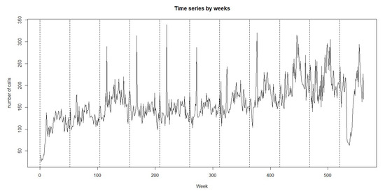
Figure 1.
Time series by weeks of the 83,379 emergency calls in Valencia (2010–2019).
The city has been divided into 81 neighbourhoods or districts, and the spatial distribution of the calls per district is given in Figure 2. We note a higher number of calls in central districts compared to others located outdoors of the city.
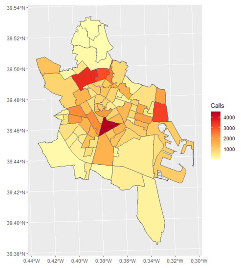
Figure 2.
Map of total number of calls per district in Valencia.
With the idea of showing some underlying aspects of the number of calls, we now show in Figure 3, Figure 4 and Figure 5 the weekly number of calls in six selected districts that we will use in the rest of the paper to show our analytical and prediction results. We show two neighbourhoods in the centre of the city (with a higher number of calls), Russafa and Sant Francesc, two neighbourhoods in the maritime east of the city, Cabanyal-Canyamelar and Malva-Rosa, and two neighbourhoods located on the outskirts of the city, one in the north, Benicalap, and one in the south, La Torre. Maritime districts highlight the effect of the arrival of tourists in summer with an increase in the number of calls. In addition, the central districts show a clear peak of calls in March due to the local festivities whose activities gather people in downtown Valencia.
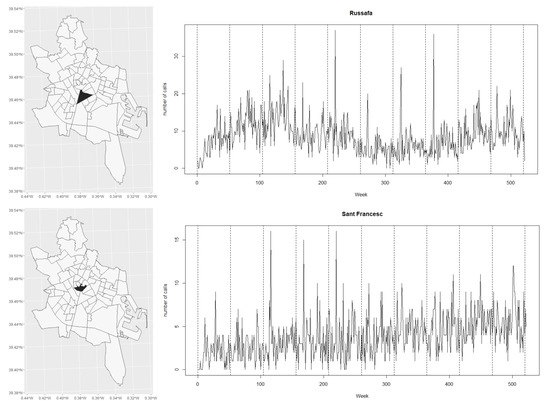
Figure 3.
Weekly calls distribution over time at central districts in Valencia, Russafa (top row), and Sant Francesc (bottom row).
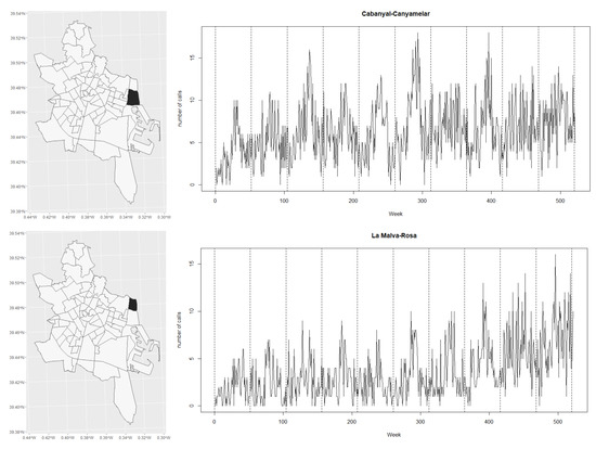
Figure 4.
Weekly calls distribution over time at maritime districts in Valencia, Cabanyal-Canyamelar (top row), and Malva-Rosa (bottom row).
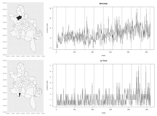
Figure 5.
Weekly calls distribution over time at Benicalap, northern Valencia (top row), and at La Torre, southern Valencia (bottom row).
To have a graphical idea of the spatial pattern of the calls due to the selected crimes, we represent such point patterns for 2012 (see Figure 6). Here, we observe an increase in calls in March and during the summer months. In addition, we can see that the increase in March happens in central districts, while the increase in calls in the summertime is more concentrated in maritime districts. For comparative purposes and to graphically analyse the space–time interaction of the calls, we also show in Figure 7 the month of January over the ten years. This graphical output shows an increasing number of calls per year for January, giving light to such dynamics and interaction in space and time.
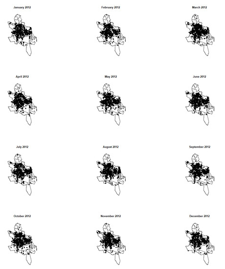
Figure 6.
Spatial point patterns of the emergency calls in Valencia for each month in 2012.
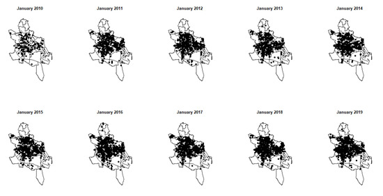
Figure 7.
Spatial point patterns of the emergency calls for the month of January of each year between 2010 and 2019.
A final piece of information we have associated with the space–time locations of the crime-related calls is based on several covariates that are minimum distances from an event (a call) to a set of selected landmarks in the city. This is highly important as different landmarks increase or decrease the number of calls, which means criminal activity can be related to being closer or further from a particular landmark. In this line, we considered the following selected landmarks or points of interest: ATMs, banks, bars, coffee shops, industries, markets, nightclubs, police stations, pubs, restaurants, and taxi stops. Furthermore, we have measured the nearest distance from a call to such landmarks. We only show some distributions and corresponding patterns for some graphical testing for brevity. Thus, on the one hand, we see how the minimum distances to restaurants or pubs (Figure 8) are dominant in the lower values of the distribution of the distances. On the other hand, in the cases of police stations or ATMs (Figure 9), the minimum distances are not that short, indicating that crimes are happening much farther from these landmarks. Finally, in the industries or markets (Figure 10), the distances seem equal or constant, indicating these landmarks have no or little effect on crimes.
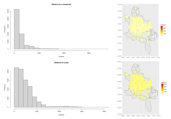
Figure 8.
Histogram and corresponding point patterns coloured by their minimum distances to restaurants (top row) and to pubs (bottom row).
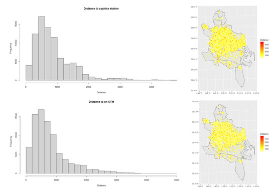
Figure 9.
Histogram and corresponding point patterns coloured by their minimum distances to police stations (top row) and to ATMs (bottom row).
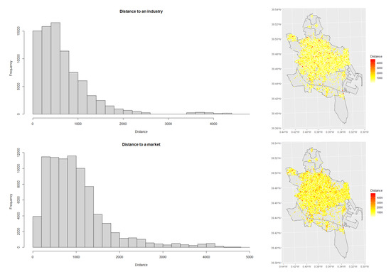
Figure 10.
Histogram and corresponding point patterns coloured by their minimum distances to industries (top row) and to markets (bottom row).
2.2. Methodology
We follow the logic of Zammit-Mangion et al. [19] to propose a suite of dynamic spatio-temporal modelling tools to identify complex underlying processes of crime data coming from calls to the emergency phone in an urban environment. Our modelling approach sits in the family of LGCP as it provides great flexibility over the more simple inhomogeneous Poisson process. Poisson point processes focus on modelling event-based data by assuming a Poisson distribution to the probability of observing a particular number of events within a defined area, D. The mean of this distribution is determined by the integral over D of an intensity function, denoted as , which is dependent on the location vector , belonging to D. A doubly stochastic or Cox process is defined if the intensity function is assumed to be a random function. In the case of a LGCP, the logarithm of the intensity is assumed to be a Gaussian process (GP), defined as a latent structure.
Let us assume we have a discrete time series of continuous spatial LGCPs, since the temporal range is discrete. Formally, let , denote a discrete time index set, and , , a set of temporally correlated spatial Gaussian processes, each with mean and covariance function . The intensity function of the point process is represented by a exponential function of for each k, i.e., . To mitigate prediction uncertainty, the mean function of can be linked to explanatory variables. In this scenario, a vector of spatially referenced covariates denoted as and its corresponding regression coefficients represented by can be employed. As such, the intensity of the LGCP at time k is given by the exponential of the sum of the regression coefficients and the mean function, i.e., .
In order to account for the intricate temporal dynamics of the intensity functions through , we adopt the stochastic integro-difference equation (SIDE) framework. This flexible modelling approach is capable of capturing dynamic temporal effects such as diffusion and dispersal. Specifically, the SIDE relates the spatio-temporal dependent variable to through the following integral equation:
where is the mixing kernel in the integral, and is an added disturbance, modelled as a Gaussian field with mean and covariance function , and D is the spatial domain under study. The non-linear mapping distorts the field in the sedentary stage; in the absence of a priori knowledge, the identity map can be adopted.
2.2.1. Correlation Analysis
We need to measure the correlation between the crime events within the same and across subsequent time frames. In point process statistics, these are quantified through the pair correlation function. Indeed, the pair auto-correlation function (PACF) , and the pair cross-correlation function (PCCF) quantify the probability of finding an event at location r given that an event has occurred at s within the same time frame k or at previous time frame . These functions are given by
where and are real and positive. The PACF determines qualitative characteristics of the events; if , no spatial pattern can be inferred from the data; and indicate event clustering and inhibition, respectively.
Given a spatial point pattern at time k, , a realisation of a particular point process model, a standard non-parametric kernel estimator of the first-order intensity is given by
where denotes the Euclidean distance on D, is an edge-correction factor, and is here representing the Epanechnikov kernel.
Consequently, non-parametric estimators of PACF and PCCF for are given by
and
where is the fraction of the circle (in two dimensions) with centre and radius lying in D.
If the processes are taken to be second-order stationary also in time, to smooth out the non-parametric estimates an average over all K time steps may be taken so that and .
Finally, note that , with ∗ being the convolution operator. The above indicates that the kernel may be acquired by performing a deconvolution on the previous equation, and conventional image processing methods such as direct inverse filtering may be applied to achieve this. Furthermore, one can show that . Note that if temporally averaged PACF/PCCFs are used, the inverse filter is given as .
2.2.2. Dimensionality Reduction
A computationally convenient truncated basis function representation of the spatio-temporal field is considered to develop an inferential approach. The choice of basis functions relies on the non-parametric estimation of the PACF. Specifically, we recall here two results. In the fundamental lemma of LGCPs, the log PACF equals the field auto-correlation function,
The second result represents the auto-correlation theorem which indicates that the spectrum of the signal is the Fourier transform of the auto-correlation function. This connection between the frequency content of the point process and the PACF is employed to pick a suitable collection of basis functions. Having the basis functions, the kernel, the mean disturbance and the field can be decomposed as
where is the vector of basis functions, and are weights which reconstruct the spatio-temporal field and the disturbance mean, respectively. Furthermore, and reconstruct the kernel covariance function and the disturbance covariance function, respectively. In this context, the SIDE of Equation (1) can be rewritten as
In this equation, and represents a Gaussian coloured noise term with a mean of and a covariance of . The objective is to estimate the unknown parameters and the states using the data , where each is a set of coordinates of the logged events at the k-th time point.
Basis Function Selection
Based on the link between the Fourier transform of the PACF and the signal spectrum, we select the collection of basis functions using a frequency-based approach. The Fourier transform of the average PACF is computed, and a cut-off frequency of cycles/unit is selected from it. Then, localised reconstruction kernels are placed at small regular intervals throughout the spatial domain. The centres of the basis functions equate the sequence of vectors defining the regular partition of length over the spatial domain D, so that
where is an oversampling parameter. Gaussianity makes mathematical development easier while still producing flexible close forms. Thus, if basis functions are defined as Gaussian radial basis functions (GRBFs) with functional form , their Fourier transforms are also Gaussian radial functions
so that the spatial and frequency variances relate through the mappings
To ensure appropriate reconstruction, the frequency and spatial range of the basis functions needs to exceed that of the field. This condition is addressed when .
Given , the previously stated relation between and can be used to find the width of the desired Gaussian radial basis functions (GRBFs), obtaining that . The resulting basis functions are a set of GRBFs with parameter placed in the spatial domain D centred on the coordinates . However, since the GRBFs are not of compact support, a compact GRBF (CGRBF) is used instead, which takes the form
for , and where denotes the Euclidean distance on D. The CGRBF is similar to the usual GRBF with but it is of compact support. The CGRBF parameter can be estimated having the GRBF parameter , or a cutoff frequency , as follows:
The cutoff frequency of is selected from the Fourier transform of the average PACF. The value corresponds to where the average PACF function decays abruptly towards zero.
2.2.3. Variational Bayesian Inference
We use the following likelihood function for inference:
where each is approximated using the same basis representation
The full posterior distribution is approximated through the variational Bayes method, and takes the form
with being the variational marginals. The variational marginals inform about important properties of the crime events’ progression. reconstructs the spatio-temporal field at every time point, shows the spatially varying escalation in events, displays the extent of the spatial dynamics, and informs about the volatility of the event occurrences. The number of unknown parameters in the reduced model scales as , where n is the number of basis functions retained.
The variational Bayes marginals for the unknown states and parameters and , with d denoting the number of covariates, can be estimated by finding the lower on the marginal likelihood. We then have
where denotes the set of variables without and is employed to compute expectations with respect to the distribution in question.
In the upcoming section, we present the method utilised to deduce the unknown variables. It should be noted that the notation denotes the estimate at time i based on the data observed until time j. For the sake of clarity, we have reformulated the model as follows: , where has a zero mean.
Parameter Estimation
Starting with the state inference, the distribution can be computed by an approximate variational Kalman smoother. Let . Considering the variational forward and backward messages, and using the Laplace method approximation, we can further write and .
The two messages are then combined to give the smoothed estimate
In relation to escalation inference, and considering the prior , its posterior can be written as
Considering now volatility inference, let the prior where denotes a Wishart distribution with V a positive definite, symmetric scale matrix and d degrees of freedom. The variational posterior can be then written as
where the evaluation of requires evaluation of the cross-covariance matrix in addition to the usual posterior covariance matrices. The computation of the cross-covariance also requires Laplace approximations.
Finally, in terms of the regression parameters, under the variational Bayes approach, we let , and set the prior . Its variational posterior is then given by
Note, finally, that the estimation of , , requires the Laplace approximation. We refer to Zammit-Mangion et al. [19] in their supplementary information for further technical details.
2.2.4. Prediction
Assuming a linear relationship from t to , the prediction of number of events for neighbourhoods and target time immediately posterior to time t is given by
where and are the estimated number of events derived from the predictive Algorithm 1, and corresponds to the number of reported events for time t and neighbourhood i.
| Algorithm 1: Prediction algorithm for time |
Number of iterations is set to L |
|
|
2.2.5. Experimental Set-Up
The VB algorithm (Algorithm 2) was assumed to have converged when the change in and , in subsequent iterations was less than 0.005, and when all diagonal elements in changed by less than . Note that the prior scale matrix and the background rate arise from the observed data itself. was chosen such that its mean is 16; this value is the squared reciprocal of the standard deviation of the week with the highest variance in the Levene’s test for homoscedasticity. In particular, was set to −4.0, indicating the expected weekly events per year. The coefficients of the covariates and their variances were initialised in 0. We set the VB algorithm to run for 200 interactions; however, it usually converged between the 50th and 65th iterations.
The exploratory analysis, VB algorithm, and predictions were implemented entirely in MATLAB R2020a. We employed parallel computing, statistics and machine learning, optimisation and mapping toolboxes, and customised functions for most of the above-mentioned methods. Further details about functions and parameters can be found in the code documentation at https://github.com/DavidPayares/ValenciaCallsSIDE (accessed on 17 January 2022). The VB algorithm was trained in a Windows CPU equipped with 16 GB RAM and 11th Gen Intel(R) Core(TM) i7 processor. Overall, the training time of the VB algorithm was 8 h and 32 min. Other methods’ computational time was negligible.
| Algorithm 2: VB-Laplace smoothers (adapted from Zammit-Mangion et al. [19]). |
Time interval = 1 is assumed throughout. Expectations are taken with respect to the relevant distributions Input: Data set , parameters , and parameter distributions . |
|
|
|
|
Output: |
3. Results
3.1. Temporal Analysis
One of the main premises of the SIDE-driven LGCPs methodology to model the temporal dynamics is that the increments between two consecutive times are normally distributed, and thus, the system can be expressed as a Geometric Brownian motion (GBM). The GBM is redefined in terms the mean and covariance function as in Equation (1). One obtains the random walk model in Equation (2) by decomposing the field . Indeed, considering that the intensity of the LGCP at time k is given by , we have , with the increment a Gaussian process with zero mean and covariance function , and a spatially varying drift.
We analysed the weekly number of emergency calls in Valencia between January 2010 and December 2019. As mentioned in the data description section, the weekly behaviour is similar yearly with a general increasing trend throughout the studied period. When we examined the increments between week N and , we found that the data’s 2.9% (12 weeks) were outliers. After removing these data, we confirmed that the increment rates between adjacent weeks were normally distributed. Figure 11 shows the distribution of the increments as well as their normal probability plot, suggesting normality in the temporal increments.
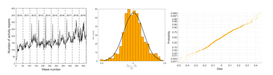
Figure 11.
Analysis of the temporal increments. The left panel displays the temporal distribution of the emergency calls over the study period (2010–2019); the central panel shows the normally-distributed weekly increments; the right panel is the normal probability plot corroborating normality in the weekly increments.
3.2. Basis Function Selection
In order to select a set of basis functions that describe the spatio-temporal field of the LGCP, non-parametric estimations of both the PACF and PCCF were conducted (see Section 3.1). Furthermore, the relationship between the PACF and PCCF is essential to determine the mixing kernel and the noise kernel (see Algorithm 3).
| Algorithm 3: Analysis for dynamic, homogeneous, isotropic spatiotemporal point processes |
|
Figure 12a shows the non-parametric estimations of both the average of (PACF) and the average of (PCCF) in terms of using the expressions in Section 3.1. Note that corresponds to approximately 270 m. Both functions are symmetric concerning zero ().
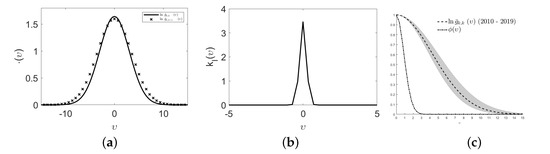
Figure 12.
Average natural logarithm PACF and average natural logarithm PCCF ((a), left plot), ((b), centre plot), cross-section on the positive real line of natural logarithm PACF, and corresponding chosen basis function ((c), right plot).
We also note that the behaviour of and are almost identical; property also noticed in Zammit-Mangion et al. [19]. Once and have been estimated, the mixing kernel and the noise kernel can be inferred using the exact inverse filter. Figure 12b shows the estimated mixing kernel of the process. This kernel should closely resemble the true underlying kernel.
Figure 12c displays a positive cross-section of and its corresponding confidence interval and that of the isotropic basis function selected for the modelling. directly comes from Equation (3) with the cut-off value obtained from the average PACF. We chose a cut-off frequency of cycles/units giving a basis parameter and an oversampling parameter of for the placement of the CGRBFs across the study area.
As in Zammit-Mangion et al. [19]’s scheme, 256 basis functions were placed on a 16 × 16 grid covering Valencia. The centre of the basis functions was separated by grid units. The functions were then filtered out to remove non-representative areas having sparse events. Only basis functions whose intensity was above a constant background event rate of (approximately five reported events per year with a distance of 450 m from its centre) and whose centre does not exceed 300 m beyond Valencia’s boundary were chosen. Figure 13 shows the distribution of reported emergency calls across Valencia and the basis functions selected for the study. In total, 129 basis functions meet the criteria; they cover the areas with high rates of emergency calls. Some areas in the northern and southern areas of the city do not have a basis function representation, given their low event rates. Nonetheless, we assigned to these areas the baseline background rate to ensure identifiability.
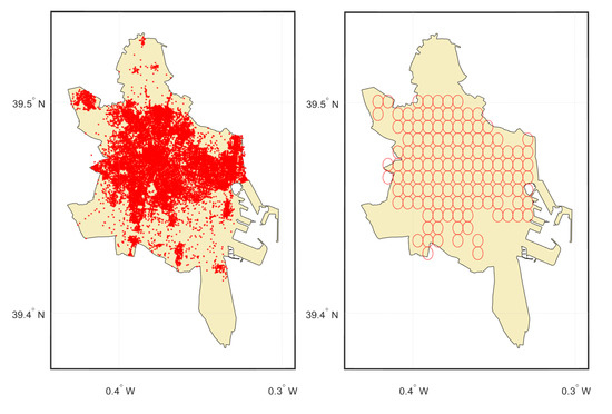
Figure 13.
Spatial locations of logged events (2010–2019), and 118 basis functions placement in the city of Valencia.
3.3. Fixed Effects
Crimes vary significantly in space and time within a region due to many demographic and economic factors, and while it is known that the combined effect of these factors favours criminal behaviour, their geographical character defines crime locations. Typically, crimes occur in business sectors within low and middle-income neighbourhoods. These sectors concentrate most of the facilities (e.g., banks, ATMs, restaurants) that compose neighbourhoods’ economic activity. Offenders target victims close to locations that can maximise their profit and reduce the risk of apprehension [20,21]. In this context, we have included putative geographical variables into the spatio-temporal point process modelling framework to measure the effect deterministic components exert on the intensity of emergency calls in Valencia.
We introduced ten covariates in the form of distances to relevant landmarks in Valencia. The landmarks included financial facilities such as banks and ATMs, and leisure places such as bars, pubs, restaurants, cafes, and nightclubs. We also included industrial areas, taxi stop areas, and markets. We measured the degree of correlation between the landmarks’ distances and the intensity of the 112 calls. Half of the covariates displayed evidence of association with the emergency calls: distance to banks, ATMs, bars, cafes, and restaurants.
Figure 14 and Figure 15 display the spatial distribution of distances to landmarks within Valencia and their relationship to the 112 calls’ intensity values. Overall, short distances to landmarks occur primarily in the city centre and densely populated neighbourhoods; facilities, shops, and venues are located strategically to provide location advantages (e.g., access to services and amenities) for residents and tourists. Distances to restaurants are short throughout the city except in the northern and part of the southwestern neighbourhoods.
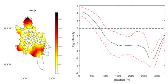
Figure 14.
Maps of fixed effects and empirical relationship between distance-based fixed effects (banks) and the log spatial intensity.
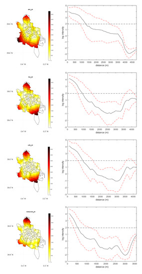
Figure 15.
Maps of fixed effects and empirical relationship between distance-based fixed effects (atms, bars, cafes and restaurants) and the log spatial intensity.
Emergency calls, which in our case reflect criminal behaviour, are known to occur frequently near facilities with features that offenders find attractive [20]; for example, places with multiple or desired targets, and our results corroborate this assumption; while the correlation between the emergency calls log intensity and the distances vary differently for each landmark, the behaviour of these relationships is relatively similar. One would expect many emergency calls in locations close to banks, ATMs, bars, cafes, and restaurants. Figure 14 shows that high intensities concentrate in a radius of approximately 1 km to 1.5 km centred in the facilities; beyond these distances, the emergency calls’ intensity decreases. We notice that the standard deviations of the correlation functions (red dotted lines) widen with distances exceeding 2 km. This occurs given the sparse number of emergency calls in low crime incidence areas.
In order to account for the factors contributing to the spatial intensity of emergency calls in Valencia, the distances to various amenities, including banks, ATMs, bars, industrial areas, markets, taxi stops, cafes, pubs, nightclubs, police stations, and restaurants were considered as the deterministic component of the intensity function . This was due to the observed strong association between these distances and the average intensity of emergency calls in the region, while we introduced eleven covariates as fixed effects in the intensity function, six presented a regression coefficient of zero. Our model could identify covariates with no quantitative influence over the emergency calls intensity. Following Algorithm 2 for inference, we found the regression coefficients for only five of the distance covariates we introduced in the intensity function; the distance to banks and ATMs parameters confidence intervals were −1.9 × 10± 1.2 × 10 and −3.4 × 10± 6.8 × 10, respectively. The results indicate that emergency calls tend to occur in proximity to economic facilities. This proximity suggests that potential perpetrators may identify victims in these areas, potentially leading to some financial gain. The regression parameters and the confidence interval for distances to bars and cafes were 0.5 × 10± 7.3 × 10 and 1.3 × 10± 7.7 × 10, respectively. In this case, emergency calls are located far from these places. It is important to note that while these types of landmarks attract a large number of potential victims, they also increase the likelihood of apprehension by law enforcement. For example, bars and cafes often have enhanced security systems due to their elevated risk of crimes, such as robbery and assault Weisburd et al. [21]. The coefficients for the distance to restaurants were found to be negative, with a magnitude of 4.0 × 10± 6.2 × 10. This suggests that emergency calls tend to occur in proximity to restaurants. This is particularly worrying, as restaurants are often targeted by criminals for robbery, burglary, and theft, due to the accumulation of significant amounts of cash during daily operations.
These results show how landmarks, to some extent, attract or repel offenders and act as proxies to identify areas with high or low emergency calls.
3.4. Heterogeneous Growth and Decay
A spatio-temporal analysis of events is concerned with identifying high-intensity spots and their evolution over space and time, and while traditional cluster analysis excels in determining hotspots, it cannot portray the temporal characteristics that govern advection and diffusion processes. Our methodology allows us not only to locate hotspots but also to determine their behaviour over time.
Figure 16 presents the weekly average fractional growth and decay of emergency calls in Valencia. As anticipated, the majority of the city has experienced a rise in the frequency of emergency calls. However, Sau Pau, Malilla, and La Torre neighbourhoods display the highest increments over the years. For example, Sau Pau is a neighbourhood prone to robbery; by 2015, it had accumulated approximately 9% of all robberies in Valencia Las Provincias [22]. Despite the fact that the central neighbourhoods of the city have the highest incidence of events, they did not exhibit a marked increase in the number of emergency calls. Conversely, areas with fewer events, such as the Quatre Carreres district, have experienced an increase in emergency call hotspots over the course of the study period. The spatial intensity of emergency calls has shown a decrease in certain areas throughout Valencia. An interesting finding is the decay in the Benicalp neighbourhood. It is considered one of the most notorious neighbourhoods in Valencia due to high poverty levels, illegal occupation, and drug traffic, and while criminal activity has grown consistently in this neighbourhood over the last few years, the number of reported emergency calls has decreased. A possible explanation is that victims or witnesses do not report crimes as they are afraid of repercussions by organised crime. Other neighbourhoods, such as La Punta and El Castellar, also display a reduction in hotspots. However, volatility (Figure 17) suggests that the data in these areas are not very reliable.
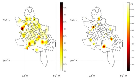
Figure 16.
Posterior mean fractional growth (left panel) and (right panel) decay of emergency calls per week in Valencia (2010–2019).
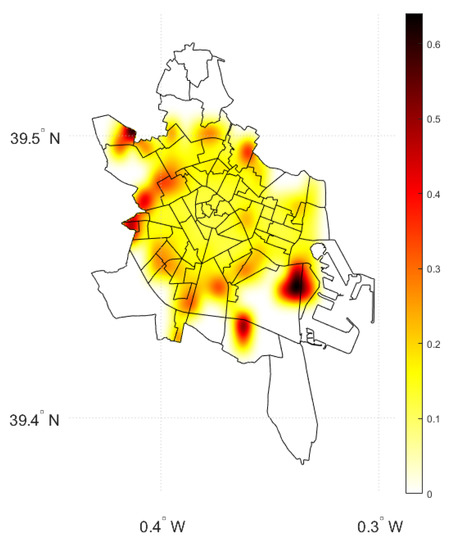
Figure 17.
Volatility map in emergency calls in Valencia (2010 to 2019).
3.5. Volatility
The volatility () in the SIDE-driven LGCP allows us to measure the accuracy of future intensity estimations. The lower the value in the diagonal of , the more accurate the predictions are, and conversely. Figure 17 shows the volatility map for emergency calls in Valencia. High volatility is present in the neighbourhoods of La Punta, Benimamet, La Llum, and Castellar-L’Oliveral. In both Banimamet and La Llum, the volatility is high as the neighbourhoods reported zero emergency calls in most of the weeks of the study. This produces a volatile temporal trend fluctuating between zero and the number of logged events (e.g., La Llum reported a maximum of four events per week) that the model cannot capture, while La Punta and Castellar-L’Oliveral also report many weeks with zero observations, high volatility results from scattered events in both time and space. For example, emergency calls in La Punta are primarily located close to the boundary with adjacent neighbourhoods. The majority of the city displays low volatility values, particularly areas with generous data, such as the city centre and surrounding neighbourhoods. The volatility map suggests that we will obtain less accurate predictions as we move from the city centre towards the suburbs.
3.6. Model Fitting
We perform model parameter estimation through Bayesian inference as detailed in Section 2.2.3, and using Algorithm 2. In particular, we estimate the intensity quartiles through the posterior smoothed estimate, the smoothed covariance matrix, and the effect of the covariates. Figure 18 shows the fitted model for five different neighbourhoods in Valencia. Overall, the model fits the data well. Real values are essentially contained in the 90% confidence intervals except in weeks when the number of reported emergency calls drops down to zero, as in La Malva-Rosa neighbourhood. The model also captures the temporal trend of the events, in some cases, even when abrupt spikes occur. An example is the neighbourhood of Arrancanpins, whose events count shot up from 9 calls in week 376 to 66 in week 377. The model accurately imitates this peak.
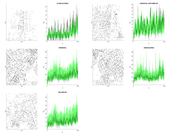
Figure 18.
Model fitting for five different neighbourhoods in Valencia. For each neighbourhood, the left panel shows the spatial distribution of the emergency calls with a buffer of 100 m, and the right panel displays the weekly counts (black) with their corresponding 90% fitted confidence intervals (green).
How accurately the model fits the data varies according to the weekly changes and the overall temporal trend. The larger the shifts from week to week are, the narrower the bandwidths become. Nonetheless, generally, the model fairly reconstructs the spatial and temporal character of the reported emergency calls in Valencia.
3.7. Prediction
One of the key strengths of our methodology is its ability to make predictions. Given that we have accurately modelled the spatio-temporal dynamics of emergency calls in Valencia, we can now forecast their future behaviour. To evaluate the predictive capability of the model, we used Algorithm 1 to estimate the number of emergency calls in Valencia for the first 40 weeks of 2020 (Figure 19). We selected this period aiming to assess our model’s predictive robustness. The emergency calls recorded in 2020 contrast with the training data (i.e., calls from 2010 to 2019) due to the implementation of containment measures in response to the COVID-19 pandemic. As seen in Figure 19, there was a significant decrease in emergency calls between weeks 532 and 543, which coincided with the quarantine and isolation policies imposed by the Spanish government. However, there was an increase in calls as measures were relaxed. We expect our method to be robust enough to effectively model these variations based on past data, covariates, and the interaction of space and time.
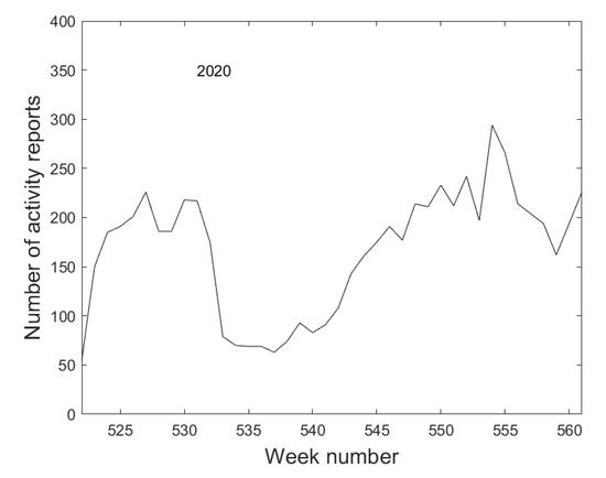
Figure 19.
Time series of the weekly calls of the first 40 weeks of 2020 in Valencia.
To stabilise the variance, we first transformed the counts into logarithms. Table 1 displays the Pearson correlation coefficients between the predicted and actual counts and log counts. These coefficients demonstrate a strong correlation between the predicted and actual values (0.87 for counts and 0.89 for log counts), indicating the model’s strong predictive ability.

Table 1.
Pearson correlation coefficients between the count and log predictions of the SIDE model and the actual values for the first 40 weeks of 2020.
The scatter plot depicted in Figure 20 presents a comparison between the logarithmic median prediction of the model and the logarithmic reported cases for the year 2020. The concentration of points around the ideal prediction line demonstrates the high level of correspondence between the predicted data and the observed data. However, it should be noted that the error bars display significant uncertainty in the median estimates for some neighbourhoods, such as Castellar-L’Oliveral and Ciutat De Les Arts I de Les Ciences. This higher level of uncertainty is likely due to the presence of multiple zero observations in these areas.
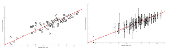
Figure 20.
Scatter plot and error bar plot between the log median predictions and log real values for 2020. The circles in the scatter plot represent individual neighbourhoods in Valencia, and the red line refers to the ideal prediction. The error bars represent the 99% confidence intervals for the predicted values.
We cannot only predict the number of emergency calls per week but also estimate their growth and decay over space and time. Figure 21 shows the histogram of the percentage of growth and decay of emergency calls for 2020. We can see that the predictions of the growth/decay rates are remarkably accurate in La Vega Baixa, Favara, La Carrasca, Ciutat Fallera, Sani Isidre, L’Hort de Senabre, and La LLum; the estimated percentage is almost identical to the observed one. These neighbourhoods are characterised by low volatility values that range from 0.01 to 0.12. The model predicts the changes with higher uncertainty in those areas with excessive zero counts (e.g., Carpesa, Exposicio, Castellar LÓliveral, and Cami Real) and, naturally, with more considerable volatility.
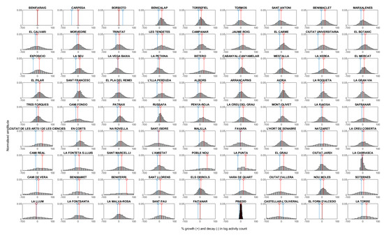
Figure 21.
Normalised histograms of log counts in 2020 per province as obtained from MC simulations with true change (circle in blue) and sample median (circle in red). The closer the blue circle is to the red circle, the most accurate is the median prediction.
While the predicted counts and change rates may vary, and in some cases, differ considerably, from the ground truth values, the model is rather accurate as (i) the predicted values are always contained in the 99% confidence intervals, (ii) the predicted log counts exhibit high correlation with the actual log counts, (iii) the distributions between the observed and predicted changes are virtually analogous, and (iv) predicted values come with a measurement of uncertainty.
Comparison with Alternative Benchmark Models
In order to evaluate the predictive capability of our model, a comparison was conducted between using its logarithmic predictions and those generated by three conventional and known point process modelling methods:
- (i)
- A spatial point process with a deterministic intensity function , where d(s) is a vector of spatial covariates and is the vector of corresponding regression parameters.
- (ii)
- A spatio-temporal point process with a separable and deterministic intensity function , where follows the above-mentioned structure and is a log-linear regression model in the formwith and as regression parameters, corresponding to annual periodicity, and the slope parameter overall trend.
- (iii)
- A spatio-temporal log-Gaussian Cox processes (LGCPs) with intensity function, where follows the specification in (i), is defined as in (ii), and is a second-order stationary Gaussian process with a minimally-parametrised exponential covariance function.
The results of this comparison provides valuable insights into the strengths and limitations of our model, as well as its overall performance in the prediction of point process data. Further details on the models are described in [15,23,24].
We assessed the four models using the mean squared prediction error (MSPE) and the Pearson correlation () between the log predicted counts and the log real counts. The results are presented in Table 2. Note that the spatio-temporal LGCP coupled with the SIDE framework displays the lowest MSPE and the highest . As expected, the purely spatial point process model displayed the poorest assessment metrics, due to the absence of the temporal component in the intensity function modelling. The spatio-temporal point process model and the spatio-temporal LGCP model showed similar metrics, with the latter being a superior alternative. Despite the relatively good performance of the benchmark models, they were unable to compete with our approach.
Table 2.
MSPE and Pearson correlation coefficients between the log real counts and log predictions of benchmark models and our method for the first 40 weeks of 2020.
The computation of models (i) and (ii) was straightforward as did not entail the use of Monte Carlo simulations. The estimation of model (iii), on the other hand, was performed using the lgcp R package, with a processing time of 3 h and 45 min. Despite the prolonged processing time of our approach compared to other available models, the results exhibit a substantial increase in prediction accuracy. This trade-off between processing time and accuracy is justified, as the primary objective of point process models is to accurately forecasts future events in space and time.
4. Conclusions and Discussion
Nowadays, technology makes enormous amounts of data readily available to researchers, and being able to handle such large quantities of information provides a step forward in many societal problems. One such problem is considered here as emergency calls in an urban context. Authorities must allocate resources and infrastructure for an effective response, identify high-risk event areas, and develop contingency strategies. We highlight that such emergency calls’ spatial and temporal analysis is crucial to understanding and mitigating distress situations.
We have proposed a modelling framework to handle heterogeneous, dynamic, and complex underlying processes to observe crime-related emergency calls. Our strategy can account for the intrinsic complex space–time dynamics by handling complex advection, diffusion, relocation, and volatility processes. This is shown by analysing the dynamics of some emergency calls in Valencia, Spain, for ten years (2010–2029), and we believe this is a case study that can be an excellent example for many similar emergency calls in other urban contexts.
For example, other more complex scenarios can be idealised in our framework by considering SIDE with a non-linear transformation of the random field at time k in the integrand of our SIDE equation. This would complicate the model while providing a more flexible case. A combination with some deep learning methods could be imagined here. This can be the motivation for further research.
There are, however, some limitations due to the baseline assumptions imposed in the modelling approach. Note that the SIDE-driven LGCPs methodology sits on the assumption that the increments between two consecutive times are normally distributed, and thus, the system can be expressed as a Geometric Brownian motion. This must be verified a priori, and thus we can not expect that all types of data behave this way. Another sort of computational disadvantage is that the procedure involves a large number of matrix inverse calculations that can bring trouble in cases where the determinants are close to zero.
The code used in this paper has been made publicly available on the authors’ Github repository (https://github.com/DavidPayares/ValenciaCallsSIDE) (accesed date on 17 January 2022). The authors have translated the LGCP + SIDE methodology into easily understandable and executable scripts, which not only replicate the results reported in this paper but also facilitate its implementation with similar datasets. The availability of the code enhances the reproducibility and transparency of the research findings.
Author Contributions
Conceptualization, J.M.; Methodology, D.P.-G. and J.M.; Software, D.P.-G.; Validation, D.P.-G. and J.M.; Formal analysis, D.P.-G. and J.M.; Data curation, J.P.; Writing—original draft, D.P.-G. and J.P.; Writing—review & editing, D.P.-G. and J.M.; Visualization, J.P.; Supervision, J.M. All authors have read and agreed to the published version of the manuscript.
Funding
This research received no external funding.
Institutional Review Board Statement
Not applicable.
Informed Consent Statement
Not applicable.
Data Availability Statement
Data sharing is not applicable to this article.
Conflicts of Interest
The authors declare no conflict of interest.
Appendix A. Literature Review Table
Table A1.
Literature review of spatio-temporal models for analysing and predicting emergency calls.
Table A1.
Literature review of spatio-temporal models for analysing and predicting emergency calls.
| Authors | Method | Contribution |
|---|---|---|
| Hashtarkhani et al. [2] | GIS | Spatial and temporal analysis of emergency calls in Iran |
| Sabet et al. [3] | GIS and Kernel estimation | Spatio-temporal insights of emergency response by fire departments in Canada |
| Towers et al. [4] | Linear regression | Forecast of future emergency events and determination of driving factors in Chicago, USA |
| Cramer et al. [5] | Hotspot analysis and Geographically weighted regression | Spatio-temporal analysis of 911 calls in Oregon, USA |
| Chohlas-Wood et al. [6] | Rolling Forecast Prediction Model | Temporal analysis and forecasting of 911 calls in New York City |
| Marco et al. [7] | Poisson log-linear mixed model | Spatio-temporal mapping of suicide-related emergency calls |
| Robles et al. [8] | Bivariate–Gaussian kernel, decision tree learning, random forest, and logistic regression | Spatio-temporal relations to predict 911 events in Cuenca, Ecuador |
| Zhou et al. [9] | Geographically weighted regression | Estimation of the spatial distribution of urban populations based on first-aid calls based in Shanghai, China |
| Heaton et al. [10] | Inhomogeneous Poisson point process | Inference of number and type of 911 calls in Houston, USA |
| Li et al. [11] | Non-parametric self-exciting point processes | Spatio-temporal modelling of emergency calls in Pennsylvania, USA |
References
- Dunnett, S.; Leigh, J.; Jackson, L. Optimising police dispatch for incident response in real time. J. Oper. Res. Soc. 2019, 70, 269–279. [Google Scholar] [CrossRef]
- Hashtarkhani, S.; Kiani, B.; Mohammadi, A.; MohammadEbrahimi, S.; Eslami, S.; Tara, M.; Matthews, S.A. One-year spatiotemporal database of Emergency Medical Service (EMS) calls in Mashhad, Iran: Data on 224,355 EMS calls. BMC Res. Notes 2022, 15, 8. [Google Scholar] [CrossRef]
- Sabet, M.S.; Asgary, A.; Solis, A.O. Emergency calls during the 2013 southern Ontario ice storm: Case study of Vaughan. Int. J. Emerg. Serv. 2019, 8, 292–314. [Google Scholar] [CrossRef]
- Towers, S.; Chen, S.; Malik, A.; Ebert, D. Factors influencing temporal patterns in crime in a large American city: A predictive analytics perspective. PLoS ONE 2018, 13, e0205151. [Google Scholar] [CrossRef]
- Cramer, D.; Brown, A.A.; Hu, G. Predicting 911 Calls Using Spatial Analysis. Softw. Eng. Res. Manag. Appl. 2012, 2011, 15–26. [Google Scholar]
- Chohlas-Wood, A.; Merali, A.; Reed, W.; Damoulas, T. Mining 911 Calls in New York City: Temporal Patterns, Detection, and Forecasting. In Proceedings of the AAAI Workshop: AI for Cities, Austin, TX, USA, 25–26 January 2015. [Google Scholar]
- Marco, M.; Lopez-Quilez, A.; Conesa, D.; Gracia, E.; Lila, M. Spatio-Temporal Analysis of Suicide-Related Emergency Calls. Int. J. Environ. Res. Public Health 2017, 14, 735. [Google Scholar] [CrossRef]
- Robles, P.; Tello, A.; Zuniga-Prieto, M.; Solano-Quinde, L. Modeling 911 Emergency Events in Cuenca-Ecuador Using Geo-Spatial Data. In Proceedings of the 4th International Conference on Technology Trends (CITT), Babahoyo, Ecuador, 29–31 August 2018. [Google Scholar]
- Zhou, Y.; Zhu, Q.Z.; Luo, L. Simulation of the spatial distribution of urban populations based on first-aid call data. Geospat. Health 2020, 15, 267–273. [Google Scholar] [CrossRef]
- Heaton, M.J.; Sain, S.R.; Monaghan, A.J.; Wilhelmi, O.V.; Hayden, M.H. An Analysis of an Incomplete Marked Point Pattern of Heat-Related 911 Calls. J. Am. Stat. Assoc. 2015, 110, 123–135. [Google Scholar] [CrossRef]
- Li, C.; Song, Z.; Wang, X. Nonparametric Method for Modeling Clustering Phenomena in Emergency Calls Under Spatial-Temporal Self-Exciting Point Processes. IEEE Acces 2019, 7, 24865–24876. [Google Scholar] [CrossRef]
- Mohler, G.O.; Short, M.B.; Brantingham, P.J.; Schoenberg, F.P.; Tita, G.E. Self-Exciting Point Process Modeling of Crime. J. Am. Stat. Assoc. 2011, 106, 100–108. [Google Scholar] [CrossRef]
- Reinhart, A. A Review of Self-Exciting Spatio-Temporal Point Processes and Their Applications. Stat. Sci. 2018, 33, 299–318. [Google Scholar]
- Shirota, S.; Gelfand, A.E. Space Furthermore, Circular Time Log Gaussian Cox Processes with Application To Crime Event Data. Ann. Appl. Stat. 2017, 11, 481–503. [Google Scholar] [CrossRef]
- Diggle, P.J.; Moraga, P.; Rowlingson, B.; Taylor, B.M. Spatial and spatio-temporal log-gaussian cox processes: Extending the geostatistical paradigm. Stat. Sci. 2013, 28, 542–563. [Google Scholar] [CrossRef]
- Shirota, S.; Banerjee, S. Scalable inference for space-time Gaussian Cox processes. J. Time Ser. Anal. 2019, 40, 269–287. [Google Scholar] [CrossRef]
- Tang, Y.; Zhu, X.; Guo, W.; Ye, X.; Hu, T.; Fan, Y.; Zhang, F. Non-Homogeneous Diffusion of Residential Crime in Urban China. Sustainability 2017, 9, 934. [Google Scholar] [CrossRef]
- Short, M.B.; D’Orsogna, M.R.; Pasour, V.B.; Tita, G.E.; Brantingham, P.J.; Bertozzi, A.L.; Chayes, L.B. A statistical model of criminal behavior. Math. Model. Methods Appl. Sci. 2008, 18, 1249–1267. [Google Scholar] [CrossRef]
- Zammit-Mangion, A.; Dewar, M.; Kadirkamanathan, V.; Sanguinetti, G. Point process modelling of the Afghan War Diary. Proc. Natl. Acad. Sci. USA 2012, 109, 12414–12419. [Google Scholar] [CrossRef]
- Eck, J.E.; Clarke, R.V.; Guerette, R.T. Risky Facilities: Crime Concentration in Homogeneous Sets of Establishments and Facilities. In Imagination for Crime Prevention: Essays in Honour of Ken; Lynne Rienner Publishers: Boulder, CO, USA, 2007; Volume 21, pp. 225–264. [Google Scholar]
- Weisburd, D.; Groff, E.R.; Yang, S.M. The Criminology of Place: Street Segments and Our Understanding of the Crime Problem; Oxford University Press: Oxford, UK, 2013. [Google Scholar]
- Las Provincias. Valencia Neighborhoods With Highest Thefts Incidence. Las Prov. 2017. [Google Scholar]
- Diggle, P.; Rowlingson, B.; Su, T.L. Point process methodology for on-line spatio-temporal disease surveillance. Off. J. Int. Environmetr. Soc. 2005, 16, 423–434. [Google Scholar] [CrossRef]
- Taylor, B.M.; Davies, T.M.; Rowlingson, B.S.; Diggle, P.J. Lgcp: Inference with spatial and spatio-temporal log-gaussian cox processes in R. J. Stat. Softw. 2013, 52, 1–40. [Google Scholar] [CrossRef]


Disclaimer/Publisher’s Note: The statements, opinions and data contained in all publications are solely those of the individual author(s) and contributor(s) and not of MDPI and/or the editor(s). MDPI and/or the editor(s) disclaim responsibility for any injury to people or property resulting from any ideas, methods, instructions or products referred to in the content. |
© 2023 by the authors. Licensee MDPI, Basel, Switzerland. This article is an open access article distributed under the terms and conditions of the Creative Commons Attribution (CC BY) license (https://creativecommons.org/licenses/by/4.0/).