A Joint Allocation Method of Multi-Jammer Cooperative Jamming Resources Based on Suppression Effectiveness

Abstract

This paper studies the resource allocation problem when multiple jammers follow the aircraft formation to support ground penetration. A joint optimization allocation method of multi-jammer beam-power based on the improved artificial bee colony (IABC) algorithm is proposed. The air-to-ground “many-to-many” assault of the multi-jammer cooperative suppression jamming model is given. The constant false alarm probability detection model of the networked radar is used to evaluate the suppression effect, and a coordinated control model of multi-jammer jamming beams and emitting power is established. The optimal allocation scheme under different combat scenarios is solved by using the IABC algorithm. The search efficiency of the ABC algorithm is improved by cross mutation operation and the replacement of the worst nectar source, and the search performance of the algorithm is enhanced by the random key encoding. Due to the infeasible solution generated by the special random key encoding method, the feasible adjustment strategy is adopted. By changing the jamming parameters, the effect on the detection probability of the radar network is analyzed. Compared to the GWO, SCA, BBO and ABC algorithms, the jamming resource allocation scheme obtained by the proposed IABC algorithm makes the radar detection probability lower. The IABC algorithm has better global search capability and robustness.

1. Introduction

When airborne formations are conducting air-to-ground assault electronic jamming missions, the form of confrontation is no longer the traditional “one-to-one” and “many-to-one” but the “many-to-many” confrontation [1,2,3]. The jamming target transformed from a single radar to networked radars. The networked radar can collect, integrate and utilize the resources and information advantages from each radar resulting in the traditional single jammer mode being less effective in jamming. Multi-jammer cooperative jamming has the following advantages when countering networked radars [4]: (1) The jammers have a wide distribution range, which is easy to realize the main lobe jamming; (2) the hardware has low jamming power standard; (3) deception jamming can generate false tracks; and (4) the system is highly flexible, and the jamming beam can be controlled in coordination. Therefore, the multi-jammer cooperative jamming technology for networked radars has become the current trend. The reasonable configuration of jamming resources can avoid the waste of jamming resources and improve their utilization. Especially for a large-scale radar network, how to maximize the jamming effectiveness of the limited jamming resources requires scientific and reasonable resource allocation. Many factors should be taken into consideration in jamming resources allocation, such as jamming beam, transmission power, frequency band and time, and so on. It is difficult to realize parallel allocation of multiple resources in algorithm design. The quality of the distribution scheme needs to be evaluated using reasonable indicators. Designing a more advantageous resource allocation algorithm to improve jamming efficiency is a problem worthy of further study.

After obtaining the operating parameters of the ground radar, reasonable allocation of the jamming resources can effectively improve the jamming efficiency and reduce the detection performance of the network radar. This paper starts with the decision of jamming resource allocation, taking multiple jammers following aircraft formations to penetrate ground netted radars as the combat scenario, and researches the problem of cooperatively suppressing jamming beams and power allocation during the assault process. This study makes important contributions to the paper. These are summarized below:

• The radar detection performance change is regarded as an indicator to evaluate the jamming suppression effect, and the influence of different cooperative jamming methods on the radar detection probability are discussed. A calculation model for the detection probability of networked radars under cooperative jamming is proposed.
• A powerful variant of the ABC algorithm is proposed to improve the adaptability and performance of the algorithm. The IABC algorithm is proven to be effective by comparing it with different heuristics.
• The proposed IABC algorithm is improved by using crossover mutation operation, a mechanism for replacing the worst nectar, and random key encoding.
• This problem focuses on the dynamic allocation of two variables, including jamming beam and power. In order to compute the distribution scheme of multiple resources in parallel, we apply a random key encoding method. A random integral and a random deviation are mapped to jamming beam pointing and the proportion of power, respectively. In addition, a repair strategy for infeasible solutions is designed to ensure that all solutions in the iteration meet complex constraints.

The rest of the paper is organised as follows: Current related work is summarised in Section 2. The jamming beam and power joint allocation model design and problem formulation are in Section 3. The detailed IABC algorithm is described in Section 4. The simulation is shown and the results are discussed regarding the performance evaluation of the IABC algorithm in Section 5. Finally, we conclude this paper in Section 6.

2. Related Work

At present, domestic and foreign research on resource allocation of multi-jammer coordinated jamming mainly focuses more on how to determine the jamming correspondence between multiple jammers and each member radar of the netted radar. Pan et al. [5] studied the multi-jammer cooperative noise jamming radar network and established the task assignment of the jammers throughout the entire course under a fixed track. Cui et al. [6] constructed a target threat level evaluation model and proposed a resource allocation model that adaptively adjusts the number of beams, which realized the resource allocation of ground-to-air multi-beam radar jamming systems that interfere with multiple targets at the same time. Song et al. [7] established a jamming task request model based on neurons. To improve the effectiveness of the multi-beam jamming system, the radar is classified and the jamming tasks are integrated to obtain an effective resource allocation plan. Gao et al. [8] divided the jamming airspace into several irradiation space, and allocated power to the targets irradiated by the beam according to the threat level. Wan et al. [9] combined the extended model of the Lanchester square law with variable efficiency factor, assuming that the total power of the jammer is fixed and proposed a method of co-jamming power allocation based on constant power. Liu et al. [10] and Li et al. [11] studied the problem of power allocation when a single jammer interferes with a radar network. He et al. [12] studied the power coordinated jamming of multiple jamming stations on the ground to airborne radar from the signal. By controlling the phase relationship of each transmitted signal, the jamming power combination was realized, and the result showed that the effective suppression area was enlarged. The above research only optimizes the allocation of single type jamming resources, but the joint optimization of multi type jamming resources is more meaningful in the actual mission requirements. Zhang et al. [13] takes the detection probability of the netted radar to the aircraft as the jamming effectiveness index and takes into account the generalization error of the detection probability caused by the uncertainty of the radar system parameters and obtains a more robust jamming beam and transmit power resource optimization model. However, the method proposed in this paper does not realize the parallel optimization of jamming resources, and the two-step optimization method is used to allocate the beam and power respectively. Cheng et al. [14] deduced the calculation model of radar exposure area under multi-UAV suppression jamming. The model showed that the jammer power, the distribution azimuth and the jammer’s main beam direction will all affect the radar detection area.

The effectiveness evaluation index of the jamming system is the basis for implementing resource allocation. From the perspective of the interfered party, the tactical performance change after the radar is interfered is mainly used as the evaluation index. Zhu et al. [15] has modeled and analyzed the radar detection range under jamming conditions and can calculate the jamming distance of self-defense jamming and long-range support jamming. Hou et al. [16] obtained high-precision radar detection probability calculation models for fixed and moving targets, fast and slow fluctuating targets with and without jamming. Liu Xiang [4] carried out a detection-level cooperative jamming study based on suppression effect and analyzed the suppression effect on OS-CFAR radar detectors under different cooperative jamming methods under the condition of radar site errors. The detection probability model of the networked radar is proposed to perform quantitative simulation analysis on the suppression effect.

For the optimization solution of the jamming resource allocation problem, the mathematical programming methods in traditional operational research can be used, such as the Hungary algorithm, Greedy algorithm, Technique for Order Preference Similarity to Ideal Solution, etc. [17]. However, due to the high nonlinearity of the objective function and the huge amount of searching in the high-dimensional solution space, the above methods are not effective. Meta-heuristic algorithm is not limited to the type of optimization problem and is less affected by the initial value. It can solve non-continuous and non-differentiable problems. The BBO algorithm was used to solve the fire resource allocation by Luo et al. [18]. However, BBO is highly dependent on migration and mutation operations, resulting in strong exploitation and weak exploration. Xing et al. [19] studied the target allocation problem of the jammer to the radar by designing the GWO algorithm, which did not involve the joint optimization of the jamming beam and power multiple resources. In addition, the dynamic allocation problem under complex constraints was not studied in the above references. The sine cosine algorithm (SCA) is a novel stochastic optimization algorithm. The algorithm has a simple structure and is easy to implement, but also suffers from the disadvantages of early convergence and low accuracy [20]. The artificial bee colony algorithm has the advantages of strong global search capability, less likely to fall into local optimum, and fewer algorithmic variables. Li verified its wide applicability in several fields, especially its effectiveness in solving combinatorial optimization and dynamic scheduling problems [21]. Therefore, according to the characteristics of the studied problem, we make an adaptive improvement of the ABC algorithm to achieve the joint allocation of jamming resources.

3. Multi-Jammer Cooperative Jamming Networked Radar Beam-Power Joint Allocation Model

3.1. A Framework for Joint Allocation of Jamming Beam-Power

During mission execution, the jammer conducts battlefield electromagnetic situational awareness by interacting with the environment. The decision layer preprocesses mission information. The allocation layer receives commands from higher decision-making units to generate jamming resource allocation solutions. The control layer generates control commands and performs jamming actions.

Figure 1 depicts two calculation processes for jamming resource allocation. Since the beam allocation and power allocation of the jammer are coupled, a tandem structure which simply connects these two problems is disadvantageous and may affect the performance of the allocation solution. However, the parallel structure computing allocation scheme can achieve global optimization, especially with limited jamming resources. The parallel structured processing flow proposed in this paper realizes the joint beam and power allocation.

3.2. Jamming Beam-Power Allocation Constraint Model

Suppose that, in a certain air-to-ground assault mission, the radar network consists of N ground-based radars $\{R_1,R_2,\dots ,R_N\}$, there are air formations composed of Q potential air targets $\{S_1,S_2,\dots ,S_Q\}$, and M jammers $\{J_1,J_2,\dots ,J_M\}$ are deployed to perform coordinated jamming missions to cover the aircraft’s assault.

3.2.1. Beam Allocation Constraint Model

Figure 2 is a schematic diagram of a multi-jammer cooperative jamming networked radar. It is stipulated that each beam can only jam one radar, and each radar can be interfered by multiple beams. The beam pointing vector of the jammer m at time k is ${\mathit{d}}_k^m=[d_{m,1,k},d_{m,2,k},\cdots ,d_{m,N,k}]$, where $d_{m,n,k}\in \left\{0,1\right\}$ is the decision variable. If $d_{m,n,k}=0$, it means that the jammer m has not allocated beams to radar n; if $d_{m,n,k}=1$, it indicates that the jammer m allocates beams to radar n.

Assuming that the jammer m can generate ${\eta }_m$ beams, it is stipulated that a jamming beam can only point to one radar at time k. To prioritize as many radars as possible to be jammed, it is stipulated that under unsaturated jamming conditions, that is, when the number of beams generated by the entire jamming system is less than the number of radars, a given radar can only receive at most one jamming beam signal. However, under saturated jamming conditions, that is, when the number of beams generated by the entire jamming system is larger than the number of radars, the radar must be jammed by at least one beam. The mathematical expression is shown in Equation (1).

$$\{\begin{array}{l}{\displaystyle \sum _{n=1}^N{d}_{m,n,k} }={\eta }_m, m=1,2,\cdots ,M, k=1,2,\cdots ,K,\\ 1\le {\displaystyle \sum _{m=1}^M{d}_{m,n,k} }\le {\displaystyle \sum _{m=1}^M{\eta }_m }-N+1, {\displaystyle \sum _{m=1}^M{\eta }_m }>N, n=1,2,\cdots ,N, k=1,2,\cdots ,K\\ {\displaystyle \sum _{m=1}^M{d}_{m,n,k} }\le 1, {\displaystyle \sum _{m=1}^M{\eta }_m }\le N, n=1,2,\cdots ,N, k=1,2,\cdots ,K\end{array}$$

(1)

3.2.2. Power Allocation Constraint Model

(1)

Power factor constraints

Here, jammer m has a fixed total transmit power $P_m^j$, and the jamming system can control the transmit power of the beam. The jamming power allocation decision variable can be expressed as a power factor vector as ${\omega }_k^m=[{\omega }_{m,1,k},{\omega }_{m,2,k},\cdots ,{\omega }_{m,N,k}]$, where ${\omega }_{m,n,k}$ represents the proportion of the total power of the jammer received by radar n from the jammer m at time k. The sum of the power of all the transmitted beams of each jammer is equal to the total power of the jammer, where the power factor vector is related to the beam pointing vector and satisfies the constraint condition of Equation (2).

$$\{\begin{array}{l}{\omega }_{m,n,k}>0, d_{m,n,k}=1\\ {\omega }_{m,n,k}=0, d_{m,n,k}=0\\ {\displaystyle \sum _{n=1}^N{\omega }_{m,n,k} }=1\end{array}$$

(2)

The constraint condition of jamming power allocation is expressed as Equation (3). It is worth noting that, when ${\omega }_{m,n,k}\ge 0.9$, the beam transmits the full power of the jammer, or when ${\omega }_{m,n,k}\le 0.1$, the jammer m does not assign this beam to the nth radar.

$$\{\begin{array}{l}{p}_{m,n,k}^j=0, {\omega }_{m,n,k}\le 0.1\\ p_{m,n,k}^j=P_m^j\cdot {\omega }_{m,n,k}, 0.1<{\omega }_{m,n,k}<0.9\\ p_{m,n,k}^j=P_m^j, {\omega }_{m,n,k}\ge 0.9\end{array}$$

(3)

3.3. Objective Function Model of Jamming Resource Allocation Based on Detection Probability

With regard to the establishment of jamming resource allocation models, the indicators for evaluating jamming effectiveness are also diverse due to the complexity of the counter-environment [22]. From the perspective of jammers, this paper constructs an objective function to evaluate the detection performance of networked radars, taking the detection probability of the radar to the target under the condition of suppressing the jamming as the evaluation index.

(1)

Radars are not jammed

When the radar is not interfered, the receiver input noise is internally generated thermal noise, and the average power of the equivalent input noise $N_{}^r$ is expressed as Equation (4).

$$N_{}^r=K{T}_0{B}_{r}F$$

(4)

In Equation (4), $K$ is Boltzmann’s constant (1.38 × 10⁻²³ J/K), $T_0$ is the standard temperature (290 K), $B_r$ is the noise bandwidth, and $F$ is the noise figure. The signal-to-noise ratio of the received signal of the radar n detection target q is expressed as Equation (5).

$$SN{R}_{n,q,k}=\frac{P_{n,q,k}^{rs}}{N_{}^r}$$

(5)

Here, $P_{n,q,k}^{rs}$ is reflected signal power of radar $R_n$ from target $S_q$ at time k. The detailed calculation steps are in the Appendix A.

(2)

Radars are jammed

When the radar is jammed, the input noise power of the radar receiver is the sum of the total power of the jamming signal and the internal noise power. The jamming signals emitted by the jammer are independent of each other, and the influence of the jamming signal coherence is ignored, so the jamming signal power can be linearly superimposed. Therefore, the signal-to-noise ratio of the received signal when radar n detects target q can be expressed as Equation (6).

$$SN{R}_{n,q,k}=\frac{P_{n,q,k}^{rs}}{{\displaystyle \sum _{m=1}^M\left(d_{m,n,k}\cdot P_{m,n,k}^{rj}\right)}+N_{}^r}$$

(6)

where $P_{m,n,k}^{rj}$ is jamming signal power received from the jammer $J_m$ by the radar $R_n$ at time k. The detailed calculation steps are in the Appendix A. According to the conclusion drawn from the complex derivation of the radar principle, there is a certain functional relationship among the radar detection probability and the false alarm probability and the received signal signal-to-noise ratio, but the original detection probability calculation is too complicated. In order to simplify the calculation of $P_{\mathrm{d}}$, it is assumed that all targets belong to Swerling I Type without considering the accumulation of pulses. The probability of the target q being found by radar n at time k can be approximately expressed as Equation (7).

$$P_{\mathrm{d}}{}_{n,q,k}=\exp (\frac{\alpha }{1+SN{R}_{n,q,k}})$$

(7)

$\alpha$ is the detection threshold and is a function of the false alarm probability $P_{\mathrm{fa}}$, and usually $\alpha =0.3\ln P_{\mathrm{fa}}$. The radar discovery probability can be calculated by Equations (4)–(7). It also reflects that optimizing the allocation of the beam and power of the jammers can effectively suppress the detection probability of the networked radars.

When performing the assault, the networked radars cooperate to complete the mission of detecting the target. When at least one radar has found the target, it is determined that the radar network has found the target. According to the OR criterion [4], the detection probability of the radar network for the target q at time k is expressed as Equation (8).

$$P_{\mathrm{d}}{}_{q,k}\stackrel{\mathsf{\Delta }}{=}1-{\displaystyle \prod _{n=1}^N\left(1-P_{\mathrm{d}}{}_{n,q,k}\right)}$$

(8)

4. A Beam-Power Joint Allocation Method for Multi-Jammers Cooperative Jamming Networked Radars

4.1. ABC Algorithm

The beam-power joint optimal allocation in this paper has complex constraints and is an NP-hard problem, and it is difficult to directly obtain its optimal solution, so it cannot be solved by a series of convex programming methods. Intelligent optimization algorithm is the most effective method to solve this type of model. Artificial Bee Colony Algorithm (ABC) [23,24,25] is a bionic swarm intelligent optimization algorithm based on the mechanism of nectar bee collection. The ABC algorithm has fewer parameters. The description of the algorithm is as follows: The candidate solution of the problem is regarded as a nectar source, and the bees are divided into three categories according to the division of labor, including employed bees, onlooker bees and scout bees. The employed bees are responsible for initially finding nectar sources and collecting nectar to share information. The onlooker bees are responsible for staying in the hive to collect nectar according to the information provided by the employed bees. The scout bees are responsible for randomly looking for a new nectar source to replace the original nectar source after the original nectar source is abandoned. After the bee colony and nectar source are initialized, three stages are repeatedly executed, namely the employed bee stage, the onlooker bee stage, and the scout bee stage to search for the optimal nectar source.

(1)

Population initialization

Parameter initialization. The nectar sources $\{{\mathit{X}}_1^{},{\mathit{X}}_2^{},\dots ,{\mathit{X}}_{SN}^{}\}$ are randomly generated within the feasible domain as feasible solutions, where SN is the amount of nectar, ${\mathit{X}}_i^{}={(x_i^1,x_i^2,\dots ,x_i^D)}^{\mathrm{T}}$,$x_i^j\in (L_j,U_j)$, D is the dimension of the solution vector, and $\mathit{L},\mathit{U}$ is the lower and upper bounds of the search space, respectively. Randomly generate nectar sources according to Equation (9).

$$x_i^j=x_{\min }^j+rand[0,1]\times (x_{\max }^j-x_{\min }^j). i=\{1,2, . . . , SN\} j=\{1,2, . . . , D\}$$

(9)

In Equation (9), $x_i^j$ represents the j-th dimension of the i-th nectar source, $rand[0,1]$ represents a random number of [0, 1], and $x_{\max }^j$ and $x_{\min }^j$ represent the maximum and minimum values of the j-th dimension of the nectar source, respectively.

(2)

Employed bee stage

According to Equation (10), hired bees look for new nectar sources, and evaluate the quality of nectar sources by comparing the amount of nectar (fitness function). The larger the fitness, the better the quality of the feasible solution. The employed bees select the nectar source according to the greedy mechanism and retain the nectar source with higher fitness.

$$v_i^j=x_i^j+{\varphi }_i^j(x_i^j-x_k^j), k=\{1,2, . . . , N\}$$

(10)

In Equation (10), $v_i^j$ represents the j-th dimension of the i-th nectar source after update. The disturbance amplitude ${\varphi }_i^j$ is a random number of [−1, 1], which is related to the convergence speed of the algorithm.

(3)

Onlooker bee stage

At the end of the employed bee stage, the onlooker bees select the employed bees to follow by the roulette method according to the nectar source quality, and track and develop the following nectar source. Similar to the employed bee, a local search is performed according to Equation (10) to find a new nectar source location. The algorithm also retains the better one through a greedy mechanism. The selection probability of the onlooker bee is given by Equation (11).

$$p_i=0.9\frac{F_i-F_{\min }}{F_{\max }-F_{\min }}+0.1$$

(11)

In this paper, the minimization of the detection probability is transformed into the fitness maximization of the solution. The fitness is defined as the sum of the reciprocal detection probabilities of all targets of the radar network, as shown in Equation (12).

$$\max F_{}={\displaystyle \sum _{q=1}^Q\frac{1}{P_{\mathrm{d}}{}_{q,k}}}$$

(12)

(4)

Scout bee stage

If the nectar source has not been updated when the maximum search times in adjacent domains Limit are met, the current nectar source will be abandoned. The corresponding employed bees and onlooker bees become scout bees. The algorithm enters the scout bee stage. Scout bees randomly look for new nectar sources to replace the original nectar sources through Equation (9).

4.2. Improvement of ABC Algorithm

Like many other swarm intelligence optimization algorithms, the standard ABC algorithm has the shortcomings of fall into local optimum easily in the early stage of search. Therefore, in order to enhance the local search capability of the ABC algorithm, the standard ABC algorithm is improved in this paper. Firstly, arithmetic crossover and mutation are used in the solution generation mechanisms of the employed and onlooker bee stages. An arithmetic crossover was applied between the current solution and the global best solution. Secondly, the operation of the worst nectar source replacement is performed in the scout bee stages. In addition, parallel allocation of jamming beam and power can be realized by improving the way of encoding the jamming decision matrix by distributing random keys.

4.2.1. Crossover Mutation Operation

In order to avoid falling into local optimum prematurely, crossover mutation operation is added to the algorithm to increase the diversity of solution [26], and an arithmetic crossover model is established, as shown in Equation (13). After one iteration, two nectar sources are selected for arithmetic crossover to generate two new nectar sources.

$$\{\begin{array}{l}{\mathit{X}}_A^{}=\beta {\mathit{X}}_B^{}+\left(1-\beta \right){\mathit{X}}_A^{}\\ {\mathit{X}}_B^{}=\beta {\mathit{X}}_A^{}+\left(1-\beta \right){\mathit{X}}_B^{}\end{array}$$

(13)

Here, ${\mathit{X}}_A^{}$ and ${\mathit{X}}_B^{}$ are two randomly selected nectars, and $\beta \in [0,1]$. The randomness of the population mutation allows the algorithm to escape from the local optimal solution and search for the global optimal solution. However, this randomness does not imply that the search will be in a better direction.

The element $x_i^j$ of the nectar source vector ${\mathit{X}}_i^{}$ are randomly selected for uniform mutation, and then a new nectar source ${\mathit{C}}_i={(x_i^1,x_i^2,\dots ,c_i^j,\dots ,x_i^D)}^{\mathrm{T}}$ is obtained. The mutation model is shown in Equation (14).

$$c_i^j=l_j+\mathrm{rand}\left(0,1\right)\left(u_j-l_j\right)$$

(14)

In Equation (14), $u_j$ and $l_j$ are the upper and lower bounds of the variation point, respectively. Here, $u_j=N+1$ $l_j=1$. The fitness of the nectar source position after the cross-mutation operation is evaluated, and the better solution is selected as the new generation nectar source. After crossover mutation operation, it should avoid generating infeasible solutions. For the newly generated nectar source that may not satisfy the constraint, we use the infeasible solution adjustment strategy proposed in Section 4.2.3 to ensure the feasibility of the newly generated nectar source.

4.2.2. The Worst Nectar Source Replacement Mechanism

The worst nectar source will hardly contribute to the search for the possible optimal solution, and domain exploitation of the worst nectar source will reduce the convergence speed. The OBL strategy that relies on the relative point of the generated candidate solution to replace the original candidate solution is a better estimate of the original candidate solution, which will greatly improve the convergence speed. If the worst individual elimination rule is triggered, a new nectar source is generated to replace the worst nectar source by the OBL strategy. The worst nectar location is ${\mathit{X}}_w^{}$. The new nectar location is ${{\mathit{X}}^{\prime }}_w$, and each dimension is updated as shown in Equation (15). If the fitness of the new nectar source is better than the original nectar source, replace the latter position.

$${x^{\prime }}_w^j=x_L^j+x_H^j+rand\times x_w^j, j=1,2,\dots ,D$$

(15)

4.2.3. A Random Key Based Encoding Method

The jamming beam and power parameters are coupled and the jamming beam assignment variables are discrete, so this optimization problem is a non-convex NP-hard problem [13]. A common solution is to separate the beam and power variables and convert the jamming beam to continuous variables. The original optimization problem is split into two relaxation subproblems. the ABC algorithm is not limited to the convexity and divergence of the optimization problem. The relaxation solutions of the subproblems are obtained by allocating beam and power resources in two steps, respectively. It is worth noting that the relaxed optimization problem is not equivalent to the original optimization problem, since the feasible set of the former contains the feasible set of the latter. Solving the two subproblems only generates a suboptimal solution to the original problem. In the process of encoding the jamming decision matrix, whether in the form of binary or integer encoding, the search space expands geometrically with the number of radars. In this paper, a random key is designed to encode the jamming decision matrix. The beam pointing vector belongs to a binary discrete random variable, while the power factor belongs to a continuous random variable between [0, 1]. A random key consists of two parts: A random integer of [0, N + 1] and a random deviation on the interval of [0, 1].

Assuming that the jammers have the ability to jam all radars, $\left\{{\eta }_1,{\eta }_2,\cdots ,{\eta }_M\right\}$ is the set of the number of beams generated by each jammer, the number of beams generated by the jammer m is ${\eta }_m$, the corresponding coding segment is $y_m={\left[y_1,y_2,\cdots ,y_{{\eta }_m}\right]}^T$, and $y_i$ is [1, N + 1], the random integer $floor({\mathit{y}}_m)$ of each coded segment represents the radar serial number corresponding to the jammer. The floor function $floor({\mathit{y}}_m)$ means the maximum integer vector not exceeding ${\mathit{y}}_m$. The random deviation ${\mathit{y}}_m-floor(y_m)$ relates the weight of the allocation of the jamming power. The normalised value of the random deviation belonging to a jammer is the power factor vector ${\omega }_k^m$. For example, in a certain penetration mission, three jammers interfered with six ground-based radars. It is assumed that jammers 1~3 all generate two jamming beams. Figure 3 is a schematic diagram of the encoding, which visually shows the corresponding relationship between the coding vector and the jammer beam-power allocation and defines an equal power factor line to measure the proportion of the radar-oriented transmit power to the total power of the jammer. The concise form of random key encoding effectively solves the problem of next-generation nectar source feasibility and can significantly reduce computation.

The standard ABC algorithm is generally applied into the optimization of continuous functions. If it is applied to the optimization of discrete problems, the solution obtained by the algorithm may exceed the boundaries of the constraints and the feasibility needs to be verified. Therefore, an infeasible nectar adjustment strategy is designed for initialized and newly generated nectar source that may not satisfy the constraints. In the initialization phase, a random key encoding makes all nectar feasible. If the newly generated nectar source does not satisfy the constraints after one iteration, their fitness is set to infinity according to the penalty function and the nectar source becomes the worst nectar source. The OBL strategy is used to replace the worst honey sources until the constraints are satisfied. Algorithm 1 illustrates the adjustment process of infeasible solutions.

Algorithm 1 Adjustment process of infeasible solutions

Step 1 Determine the number of radars N and encoding length D.       Initialize the population and limit the boundary conditions of the encoding.        $$\begin{gathered} \mathrm{If}D\le N \\ \hspace{1em}{\mathit{X}}_i^{}=randperm(N,D)+rand(1,D) \\ \mathrm{Else}\mathrm{if}D>N \\ \hspace{1em}{\mathit{X}}_i^{}=[randperm(N),randi([1,N],1,D-N)]+rand(1,D) \end{gathered}$$       End       End Step 2 Determine whether the updated solution satisfies the constraints.        $$\begin{gathered} \mathrm{While}{\mathit{X}}_i^{} \mathrm{is} \mathrm{not} \mathrm{feasible}. \\ \hspace{1em}F({\mathit{X}}_i^{})=0 \\ \hspace{1em}\mathrm{Replace}\mathrm{the}{\mathit{X}}_i^{} \mathrm{according} \mathrm{to} \mathrm{the} \mathrm{Equation} \left(15\right). \end{gathered}$$       End

4.2.4. The Flow of Cooperative Jamming Beam-Power Allocation Based on IABC Algorithm

The cooperative jamming beam-power allocation based on the IABC algorithm is described in Algorithm 2 and Figure 4. The main parameters of the IABC algorithm are the nectar size SN, maximum times of evaluations for fitness G_max, maximum search times in adjacent domains Limit, and the crossover and mutation probabilities. As the SN becomes larger the execution efficiency of the algorithm decreases. However, the effect of SN on the algorithm search performance cannot be described with regularity. The larger the G_max the more robust the algorithm is, but it increases the time expenditure. It should be determined depending on the specific problem. The threshold parameter Limit affects the frequency of scout bee emergence, the larger the Limit value the less frequent the scout bee emergence. The frequency of the emergence of scout bees affects the global search performance of the algorithm. The crossover and mutation probabilities affect the execution efficiency and global search performance of the algorithm. Appropriately increasing the crossover probability can improve the algorithm development ability, but too high crossover probability will result in less time for high-quality patterns to exist in the population. Conversely, there is a decrease in algorithm development capability. A larger mutation probability allows the diversity of the population to be guaranteed, but the probability of the destruction of feasible solutions increases with it, and conversely a relatively lower mutation probability prevents the population from tending to be genetically homogeneous.

Algorithm 2 Pseudo-Code of cooperative jamming beam-power allocation based on IABC algorithm

Input: Population number NP, Initial nectar number SN, Maximum times of evaluations for fitness Gmax, Maximum search times in adjacent domains Limit = 100, Dimension of Vectors D, Lower bound and Upper bound ${\mathit{L}}_j,{\mathit{U}}_j$. Output: The optimal individuals.   01: initialize population according to Algorithm 1   02: for i = 1 to SN   03: evaluate the nectar fitness   04: trial(i) = 0   04: end for;   05: while iter < Gmax   06: for each employed bee   07: obtain new solution Vi using Equation (10)   08: if Vi do not satisfy the constraints   09: Repair Vi according to Algorithm 1   10: end for   11: evaluate the fitness of Vi   12: if F(Xi) < F(Vi)   13: Xi = Vi   14: trial(i) = 0   15: end for   16: trial(i) = trial(i) + 1   17: obtain new solution Ci using Equations (13) and (14)   18: if Ci do not satisfy the constraints   19: Repair Ci according to Algorithm 1   20: end for   21: evaluate the fitness of Ci   22: if F(Xi) < F(Ci)   23: Xi = Ci   24: trial(i) = 0   25: end for   26: trial(i) = trial(i) + 1   27: iter = iter + 1   28: for each onlooker bee   29: select new solution by the roulette method   30: generate new solution Vi using Equation (10)   31: if Vi do not satisfy the constraints   32: Repair Vi according to Algorithm 1   33: end for   34: evaluate fitness value of new solution   35: if F(Xi) < F(Vi)   36: Xi = Vi   37:trial(i) = 0   38: end for   39:trial(i) = trial(i) + 1   40: iter = iter + 1   41: $\mathrm{after}\mathrm{one}\mathrm{iteration},\mathrm{replace}\mathrm{the}\mathrm{worst}\mathrm{solution}\mathrm{with}{{\mathit{X}}^{\prime }}_w$ according to Equation (15)   42: if ${{\mathit{X}}^{\prime }}_w$ do not satisfy the constraints   43: Repair ${{\mathit{X}}^{\prime }}_w$ according to Algorithm 1   44: trial(i) = 0   45: end for   46: iter = iter + 1   47: for each scout bee   48: if trial(i)> Limit   49: generate new solution Xi according to Algorithm 1   50: iter = iter + 1   51: record the optimal solution so far   52: end while

5. Numerical Simulation and Analysis

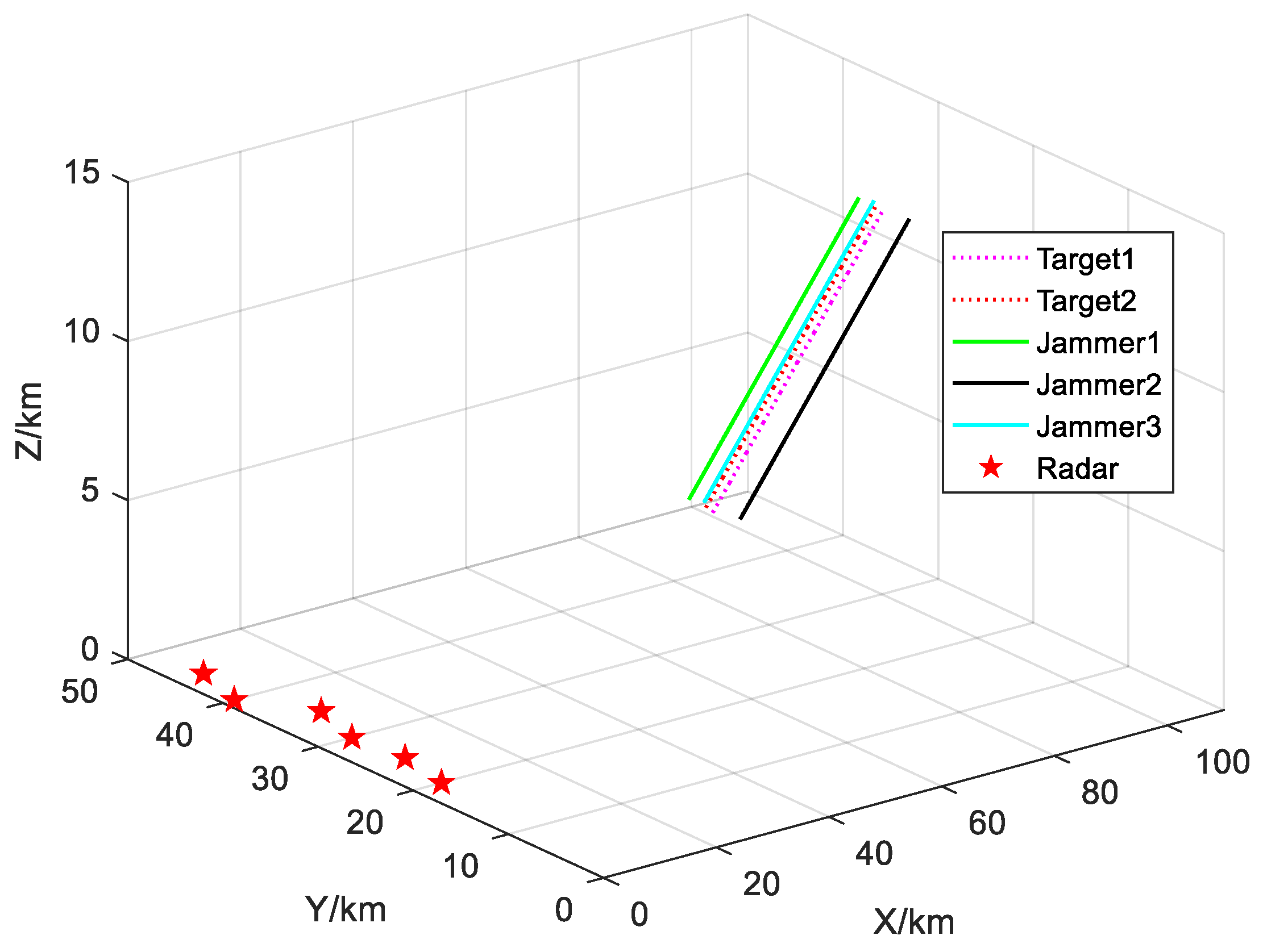
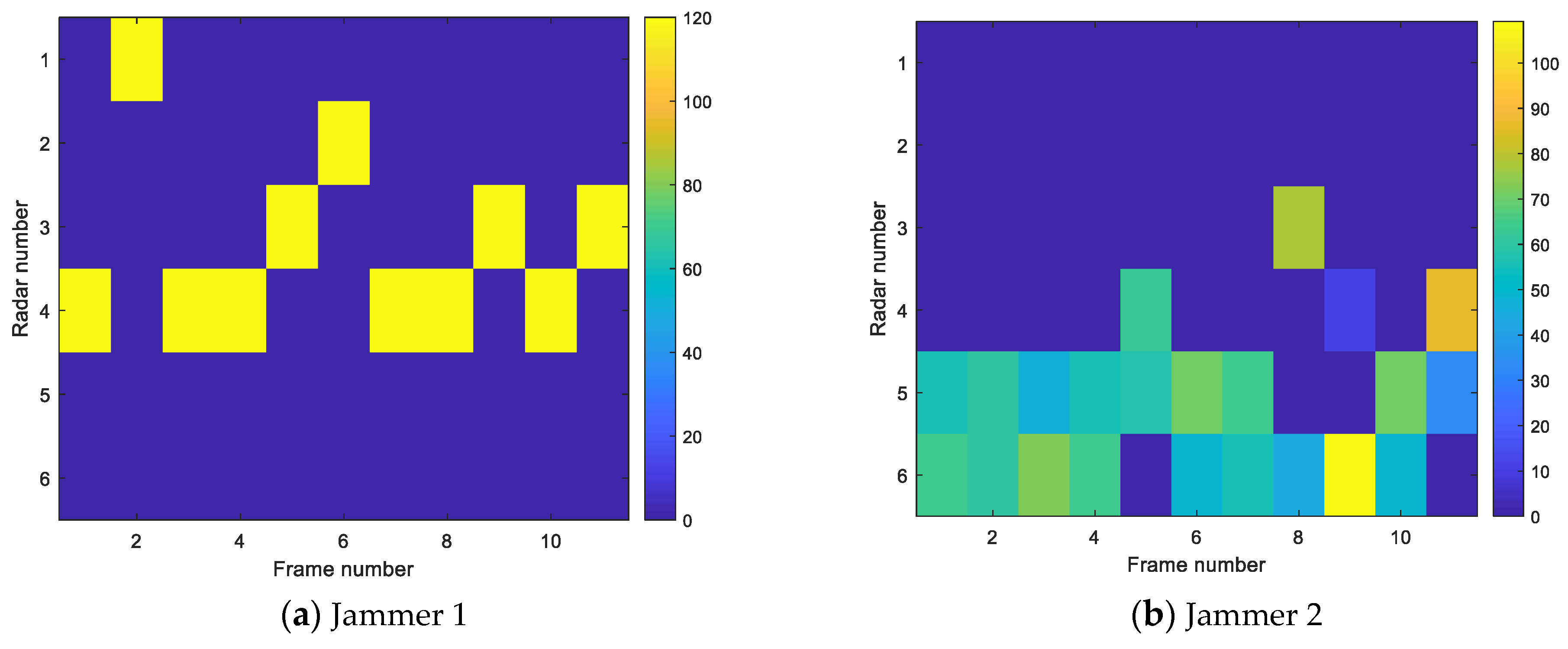
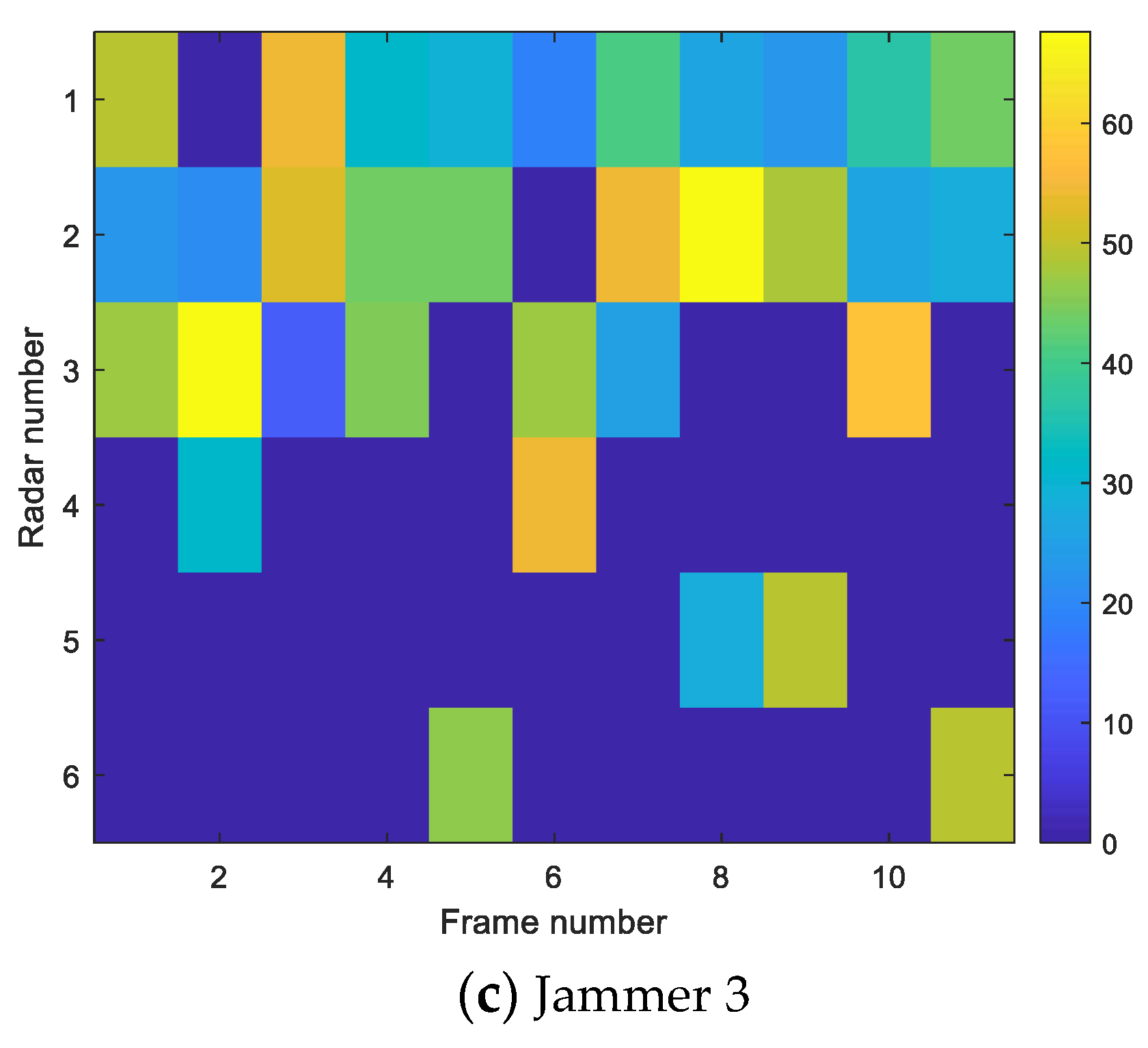
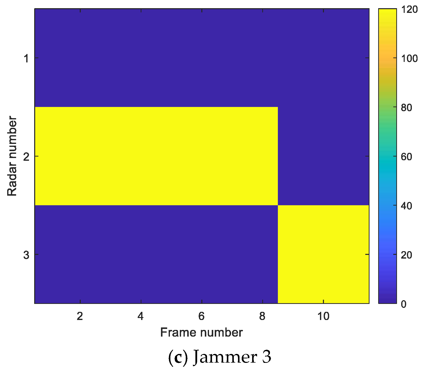
5.1. Scenario Setting and Experimental Results

Scenario 1: Suppose that there are two aircraft that assault the ground-based network radars, the number of jammers M = 3, and the number of ground-based radars N = 6. The position of radars, the initial position of the assault targets and the jammers are shown in

Table 1. Assault formation location coordinates.

	Coordinate/km
Target 1	[100, 30, 12]
Target 2	[100.5, 31, 12]
Jammer 1	[101, 33, 12]
Jammer 2	[101.5, 28, 12]
Jammer 3	[102, 32, 12]

and

Table 2. Networked radar location coordinates.

	Coordinate/km
Radar 1	[5, 20, 0]
Radar 2	[7, 25, 0]
Radar 3	[6, 30, 0]
Radar 4	[9, 35, 0]
Radar 5	[2, 40, 0]
Radar 6	[5, 45, 0]

, and the assault route of the air formation is shown in Figure 5.

The number of beams of jammers is $N_b$ = [1, 2, 3], respectively. The working index of each jammer is the same, as shown in

Table 3. Jammer working index.

Index	Value	Index	Value
$P_m^j$	120 W	${\lambda }_m^j$	0.1 m
$G_m^j$	10 dB	${\theta }_{n0.5}$	3°
$\mathsf{\Delta }{f}_m^j$	10 MHz	$L_m^j$	6 dB
${\gamma }_j$	0.5	$\left({\dot{x}}_{m,k}^j,{\dot{y}}_{m,k}^j,{\dot{z}}_{m,k}^j\right)$	[−3000, 0, −80] m/s

. The indicators of each radar are also the same, as shown in

Table 4. Radar working index.

Index	Value	Index	Value
$P_n^t$	200 MW	$F$	3 dB
$G_n^t$	40 dB	$P_{\mathrm{fa}}$	10−6
$\mathsf{\Delta }{f}_n^r$	10 MHz	${\lambda }_n^t$	0.1 m
$L_n^t$	6 dB	${\sigma }_{n,q}$	1 m2

.

The algorithm parameters stipulate: Population size NP = 40, initial nectar size SN = 20, maximum search times in adjacent domains Limit = 100, and maximum times of evaluations for fitness G_max = 100. The crossover probabilities are 0.5 and mutation is 0.05.

In the combat scenario of scenario 1, the sampling interval is 10 s, the location information and working indicators of the battlefield jammers and radars are collected, and the multi-frame battlefield situation is obtained. The simulation results of the jamming beam-power allocation under different assault situations (different frames) are as shown in Figure 6. The position of the color bar in the Figure 6 represents which radar the jammer beam points to, and the color represents the amount of power allocated by the jammer. The results show that during the entire assault period, jammer 1 allocates jamming resources to radar 1 to radar 4; jammer 2 allocates jamming resources to radar 5 and radar 6; jammer 3 mainly allocates jamming resources to radar 1 and radar 3. In addition, Figure 7 show the detection probability of the assault target by the radar network for each frame. As the aircraft formation approaches the enemy’s networked radars, the objective function optimal value decreases, the radar’s detection probability of the targets continues to increase, and the fighter’s concealment performance deteriorates. However, before t = 80 s, the detection probability of the radar to a single target is still lower than 0.5, indicating that the jamming beam-power allocation scheme has an obvious influence on suppressing effectiveness.

5.2. Comparative Analysis of Cooperative Jamming Simulation in Different Scenarios

(1)

Comparison experiment of jamming resource allocation between the multi-beam system and single-beam system

Scenario 2: Based on the settings of Scenario 1, in order to achieve saturated jamming to the radar, select jammer 1~3 to suppress radars 1~3. Jamming beam conditions: (1) Each jammer in a single-beam system can only transmit one jamming beam; (2) Each jammer in a multi-beam system can transmit two jamming beams. The rest of the parameter settings are consistent with Scenario 1. The results of beam-power dynamic allocation under each frame are shown in Figure 8 and Figure 9, respectively. In the case of single-beam and multi-beam system jamming, the detection probability curve of two targets is shown in Figure 10. Whether for assault target 1 or assault target 2, the radar discovery probability of multi-beam system jamming is lower than that of the single-beam system jamming, indicating that, when the jammer power is limited, the multi-beam system can better achieve beam and power management and maximize the effect of jamming resources.

(2)

Comparison experiment of resource allocation between saturated jamming and unsaturated jamming

In order to discuss the suppression effectiveness of jamming resource allocation, when the scale of radar network is large but there are few jammers, the effectiveness of saturated jamming and unsaturated jamming on the results of resource allocation and radar detection performance are simulated and analyzed.

Scenario 3: Jammers 1~3 suppress radars 1~6. (1) Saturated jamming condition: The total number of beams that can be transmitted by the jamming system is not less than the number of radars, so the number of beams of each jammer is L = 2. (2) Unsaturated jamming conditions: The total number of beams that can be transmitted by the jamming system is less than the number of radars, and the number of jammer beams is 1, 2, and 2, respectively. The rest of the parameters are consistent with Scenario 1.

Figure 11 and Figure 12 show the beam-power allocation results of each frame under saturated and unsaturated jamming, respectively. During the assault period, saturated jamming range can achieve full coverage of the networked radars, while unsaturated jamming can only ensure that five radars are jammed at the same time. Therefore, as shown in Figure 13, when determining the total transmitted jamming power, the saturated jamming effectiveness on the radar network is better before t = 25 s, effectively reducing the detection probability of radars, but the detection probability of saturated jamming is higher than that of unsaturated jamming after t = 25 s. This is because range is the main factor affecting the SNR. When the formation approaches the radar network during the assault, the radar reflected signal power of targets increases, and a larger jamming power is required to suppress the radar. The transmit power is distributed to each jamming beam, and saturated jamming range can cover all radars. Moreover, the formation in the early stage of assault is far away from the networked radar, and the demand for jamming power is not high, so part of the jamming power from a jammer received by a single radar in the early stage of penetration has a certain suppressing effectiveness. However, the closer the formation is to the networked radars, the greater the radar reflected signal power. Especially in the later period of assault, the jammers must transmit high-power signals to drown the reflected signals. Unsaturated jamming makes the jammer’s beam illuminate part of the radar, so that the jamming power is more concentrated and the detection performance of the entire radar network is reduced. In addition, saturated jamming has a more obvious impact on the detection performance of the networked radars than unsaturated jamming on the entire assault route.

5.3. Influence of Jamming Parameters on Detection Probability

Suppose that the number of radar networks in the new scenario increases to 10. The detection probability of the netted radar changes with the number of jammer beams and jamming transmission power. In Figure 14, if jamming beam number is less than radar number, the target will definitely be found. As all jamming systems cannot jam all radars at the same time, the jamming effect is poor. The jamming beam can cover the radar network, and the suppression effect is better. However, when the number of jamming beams exceeds 18, the results are basically unchanged. In Figure 15, when the jamming transmission power is below 50 W, the detection probabilities of the radar network for target 1 and target 2 are not less than 0.8 and 0.7 respectively. With the increase of jamming transmission power, the detection probability of the radar network decreases. When the jamming transmission power is higher than 300 W, it can ensure that the detection probability of the radar network to target 1 and target 2 is not higher than 0.7 and 0.5, respectively, and the success rate of penetration is greatly improved.

5.4. Experiment Analysis and Algorithm Performance Comparison

In order to verify the feasibility and efficiency of the improved ABC algorithm proposed in this paper, this paper compares IABC algorithm with the Grey Wolf Optimization (GWO) algorithm, sine cosine algorithm (SCA), Biogeography-Based Optimization (BBO) algorithm, and standard ABC algorithm. The algorithm parameters stipulate: population size NP = 100, maximum search times in adjacent domains Limit = 100, and maximum times of evaluations for fitness G_max = 300.

Figure 16 shows the change curve of detection probability with iteration (t = 30 s). BBO algorithm has the worst effect. The detection probability of radar network for target 1 and target 2 at t = 30 s is about 0.68 and 0.62 respectively. The IABC algorithm has the best effect, and the detection probabilities obtained under the jamming scheme are only about 0.5 and 0.37 respectively. It can be seen from Figure 17, IABC algorithm has stronger global search ability and higher robustness compared with other algorithms. For the beam and power allocation scheme, the IABC algorithm gives better results than several other algorithms and make the lowest detection probability of the radar network. Figure 18 shows the results of jamming resource allocation using the IABC method proposed in this paper.

6. Conclusions

Aiming to improve the utilization of jamming resources and to exert the maximum suppression effectiveness, the networked radar constant false alarm is established with the minimum detection probability of the networked radars to the targets as the evaluation index. Based on the probability detection model, a joint allocation method of jamming beam- power based on cooperative suppression is proposed. To improve the adaptability of the standard ABC algorithm, a random key indicating beam pointing and power occupancy is used to encode the nectar. The cross mutation operation and the worst nectar source replacement mechanism improve the global search performance and robustness of the algorithm, and an adjustment strategy is designed to handle the infeasible solutions generated after nectar update. The simulation results show that the method proposed in this paper can reasonably optimize the allocation scheme of the entire jamming system resources, effectively reduce the detection probability of the networked radar to the assault target, and the IABC algorithm has stronger global search ability than the GWO, BBO, SCA, ABC algorithm. In addition, the cooperative suppression effectiveness of single-beam system and multi-beam system under saturated and unsaturated jamming conditions is discussed and analyzed. If the total jamming power is limited, the beam-power cooperative control makes the multi-beam jamming better than the traditional single-beam jamming on the networked radar. If the jammer beam number is limited, saturated jamming in the early stage of assault can greatly reduce the radar detection performance. However, when the jammer approaches the radar in the later stage of assault, the jamming power concentration can better reduce the detection performance of a single radar. Increasing the jamming power can effectively improve the suppression effect on the radar network. When there are limited jammers, the detection probability will not decrease continuously with the increase of the number of jamming beams. The model and method proposed in this paper play a certain role in assisting the pilots to make jamming decisions when performing assault missions and realizing the intelligent decision-making of jamming resource allocation. Additionally, the IABC algorithm also has good applicability to a class of optimization problems with a combination of discrete and continuous variables. In future work, more attention will be paid to the joint allocation of jamming resources dominated by multi-objective optimization in more complex scenarios. However, the real-time and online jamming resource allocation technique is worth studying in the rapidly changing battlefield situation.

References

1. Fu, X.Y. Study on Cooperative Jamming Policy and Jamming Methods of Radar; University of Electronic Science and Technology of China: Chengdu, China, 2020. [Google Scholar]
2. Xiang, C.W.; Jiang, Q.S.; Qu, Z. Modeling and algorithm of dynamic resource assignment for ESJ electronic warfare aircraft. Command. Control. Simul. 2017, 39, 85–89. [Google Scholar]
3. Wang, X.; Fei, Z.; Huang, J.; Zhang, J.A.; Yuan, J. Joint resource allocation and power control for radar interference mitigation in multi-UAV networks. Sci. China Inf. Sci. 2021, 64, 182307. [Google Scholar] [CrossRef]
4. Liu, X. Study on Cooperative Jamming Techniques against Radar Network; National University of Defense Technology: Changsha, China, 2019. [Google Scholar]
5. Pan, Y.H.; Gao, Y.L.; Zhang, L.; Liu, W. Resource allocation optimization techniques for multi-jammer cooperative noise jamming. J. Air Force Early Warn. Acad. 2017, 31, 346–350. [Google Scholar]
6. Cui, Z.M.; Peng, S.R.; Ren, M.Q.; Long, S.M. Research on multi-beam interference resource scheduling based on beam quantity control. J. Air Force Early Warn. Acad. 2020, 34, 274–278. [Google Scholar]
7. Song, H.F.; Wu, H.; Cheng, S.Y.; Chen, Y. Integrated management algorithm of jamming resources in multi-beam jamming systems. Acta Armamentarh 2013, 34, 332–338. [Google Scholar]
8. Gao, X.G.; Hu, M.; Zheng, J.S. Jamming strategy for single plane to multi-target in task of penetration. Syst. Eng. Electron. 2010, 32, 1239–1243. [Google Scholar]
9. Wan, K.F.; Gao, X.G.; Liu, Y. Optimal power partitioning for cooperative electronic jamming based on Lanchester with variable efficiency factors. Syst. Eng. Electron. 2011, 33, 1544–1547. [Google Scholar]
10. Liu, Q.; Wang, X.H.; Wang, X.; Cheng, S.Y. A study on methods of active barrage jamming power assignment based on multi-targets. Fire Control. Command. Control. 2012, 37, 164–166. [Google Scholar]
11. Li, X.M.; Dong, T.L.; Huang, G.M. A efficient Distribution method of jamming power to distributed MIMO radar. Fire Control. Command. Control. 2017, 42, 26–31. [Google Scholar]
12. He, J.; Huang, C.; Han, G.X. Jamming blanketed zone computing model of multiple radar jammers against airborne targeting radar. Oper. Res. Manag. Sci. 2016, 25, 39–43. [Google Scholar]
13. Zhang, D.L.; Yi, W.; Kong, L.J. Optimal joint allocation of multijammer resources for jamming netted radar system. J. Or Radar 2021, 10, 595–606. [Google Scholar]
14. Cheng, Y.J.; Ma, H.; Xu, Z. Influence of distributed jamming of UAV to detecting capability of the air-defence radar. Command. Control. Simul. 2014, 36, 9–12+22. [Google Scholar]
15. Zhu, Y.; Wang, P.G.; Jiang, Z.B. Modeling and Analysis of Radar Detection Range in Jamming. Mod. Radar 2006, 28, 12–14. [Google Scholar]
16. Hou, D.Q.; Qi, F.; Yang, Z. Models for Radar Detection Probability Based on Operation Simulation. Electron. Inf. Warf. Technol. 2016, 31, 61–64. [Google Scholar]
17. Shi, R.; Liu, J. Application of Intelligent Optimization Methods in Jamming Resource Allocation: A Review. Electron. Opt. Control. 2019, 26, 54–61. [Google Scholar]
18. Luo, R.H.; Li, S.M. Optimization of Firepower Allocation Based on Improved BBO Algorithm. J. Nanjing Univ. Aeronaut. Astronaut. 2020, 52, 897–902. [Google Scholar] [CrossRef]
19. Xing, H.X.; Wu, H.; Chen, Y.; Zhang, X. Multi-efficiency optimization method of jamming resource based on multi-objective grey wolf optimizer. J. Beijing Univ. Aeronaut. Astronaut. 2020, 46, 1990–1998. [Google Scholar]
20. Yong, L.Q.; Li, Y.H.; Jia, W. Literature Survey on Research and Application of Sine Cosine Algorithm. Comput. Eng. Appl. 2020, 56, 26–34. [Google Scholar]
21. Li, C. Radar Jamming Decision Making Technology Based on Swarm Intelligence Algorithm; Xidian University: Xi’an, China, 2021. [Google Scholar]
22. Wang, B.Y. Research on the Online Effectiveness Evaluation of Radar Countermeasure; Xidian University: Xi’an, China, 2018. [Google Scholar]
23. Zorarpacı, E.; Ayşe, Ö.S. Privacy preserving rule-based classifier using modified artificial bee colony algorithm. Expert Syst. Appl. 2021, 183, 115437. [Google Scholar] [CrossRef]
24. Brajević, I. A shuffle-based artificial bee colony algorithm for solving integer programming and minimax problems. Mathematics 2021, 9, 1211. [Google Scholar] [CrossRef]
25. Yildizdan, G.; Baykan, Ö.K. A New Hybrid BA_ABC Algorithm for Global Optimization Problems. Mathematics 2020, 8, 1749. [Google Scholar] [CrossRef]
26. Sun, N.; Lu, Y. A self-adaptive genetic algorithm with improved mutation mode based on measurement of population diversity. Neural Comput. Appl. 2019, 31, 1435–1443. [Google Scholar] [CrossRef]
27. Zhou, Y.Y. Principles and Technologies of Electronic Warfare System; Publishing House of Electronics Industry: Beijing, China, 2014; pp. 130–133. [Google Scholar]
Figure 1. Jamming resource joint allocation process.
Mathematics 11 00826 g001
Figure 2. Schematic diagram of multi-jammer cooperative jamming networked radar.
Mathematics 11 00826 g002
Figure 3. Schematic diagram of random key based encoding.
Mathematics 11 00826 g003
Figure 4. Flowchart of cooperative jamming beam-power allocation based on the IABC algorithm.
Mathematics 11 00826 g004
Figure 5. Assault confrontation operation scenario.
Mathematics 11 00826 g005
Figure 6. Scheme diagram of jammer beam-power allocation to 6 radars.
Mathematics 11 00826 g006aMathematics 11 00826 g006b
Figure 7. Radar detection probability variation curve.
Mathematics 11 00826 g007
Figure 8. Beam-power allocation diagram for the multi-beam system.
Mathematics 11 00826 g008
Figure 9. Beam-power allocation diagram for the single-beam system.
Mathematics 11 00826 g009aMathematics 11 00826 g009b
Figure 10. Variation curve of detection probability of the networked radars to targets.
Mathematics 11 00826 g010
Figure 11. Beam-power allocation diagram for saturated jamming.
Mathematics 11 00826 g011
Figure 12. Beam-power allocation diagram for unsaturated jamming.
Mathematics 11 00826 g012
Figure 13. Variation curve of detection probability of networked radars to targets.
Mathematics 11 00826 g013
Figure 14. Effect of jamming beam on the detection probability of the radar network.
Mathematics 11 00826 g014
Figure 15. Effect of jamming emitting power on the detection probability of the radar network.
Mathematics 11 00826 g015
Figure 16. Convergence curves of objective functions of BBO, GWO, SCA, ABC and IABC algorithms at t = 30 s.
Mathematics 11 00826 g016
Figure 17. Change of detection probability of radar network in 100 s calculated by BBO, GWO, SCA, ABC and IABC algorithms.
Mathematics 11 00826 g017
Figure 18. Scheme diagram of jammer beam-power allocation to 10 radars.
Mathematics 11 00826 g018aMathematics 11 00826 g018b