Cash Flow Optimization on Insurance: An Application of Fixed-Point Theory

Abstract

The purpose of this paper is to explore a discrete-time cash flow optimization problem of the insurance company with time value of ruin under different interest rates. For the sake of considering the time value of ruin, we assume that the shareholders can get subsidies per unit time, as long as the insurance company is not bankrupt. The switching of different interest rates on the market is controlled by a stationary Markov chain. The dynamic programming principle is used to solve this optimization problem. By using the method of fixed-point theory, we show that the value function is the unique solution of the dynamic programming equation and a numerical algorithm is proposed to solve the value function as well as the optimal policy. Furthermore, two examples are revealed to illustrate the application of the main results obtained in the presented paper.

1. Introduction

The optimization of cash flow management has a long history in the area of actuarial science. The original study on the cash flow optimization can be traced back to 1957. At that time, De Finetti [1] proposed the maximization problem of the expected present value of the dividend payments of the insurance company. From then on, the management of cash leakages played an important role to measure the performance of the insurance company and also attracted the public attentions in the academic area. As an example, Ref. [2] considered the optimal dividend problem of diffusion process with transaction fees. Ref. [3] explored the optimal dividend pay-out optimization when the surplus follows the controlled diffusion risk model. Ref. [4] generalized the Brownian motion to the compound Poisson risk process and studied the corresponding optimal dividend with bounded dividend rate. Ref. [5] explored the optimal investment and dividend problem for the renewal process by viscosity solution approach. In the setting of continuous-time model, the dividend optimization has been investigated under various modellings in recent years. For more relevant references, one can see [6,7,8]. We also refer the reader to [9] for the exhaustive references to seek the past development on the issue of dividend optimization.

A lot of references such as [10,11] considered the optimal dividend problem under the condition that the discount factor is a constant. As we know, compared with the constant interest rate, the stochastic interest rate can simulate market changes more realistically. The optimal dividend policy with random interest rates of continuous time was studied in [12] in which the authors considered the effects of financial markets and concluded that a firm will pay more dividend if the interest rate is high and pay less dividend if the interest rate is low. Ref. [13] also considered the optimal dividend problem with stochastic interest rate while the stochastic interest rates are modelled by the geometric Brownian motion and the Ornstein–Uhlenbeck process, respectively. Moreover, the authors derived the explicit solution of the optimal strategy for the first case and switched to the viscosity solution analysis for the second case. In our paper, we also consider the optimal dividend under different interest rates.

To the best of our knowledge, compared with the continuous time model, there are fewer articles dealing with discrete time model. However, the discrete-time model’s advantage is that it is more close to the reality. In reality, all transactions are conducted on weekdays. In the setting of discrete-time model, Ref. [14] assumed that in one period the surplus risk process follows a time-homogenous Markov process with possible values $+1,0,-1,-2,\cdots$ and proved that the optimal dividend policy is of band type. Ref. [15] considered the optimal dividend of the compound binomial model with bounded dividend rate. The discrete-time dividend problem under random interest rate was studied in [16] in which the authors consider a constant penalty should be paid when the ruin occurs. Inspired by [17], instead of a ruin penalty, we consider that a subsidy must be paid to shareholders each unit time as long as the company is not bankrupt. The company aims to maximize the cumulative discounted dividends and subsidies before ruin. In our paper, we use mathematical method to explore such financial optimization problem for the insurance company.

There are various approaches to solve the optimal strategy in the field of stochastic optimal control. In our paper, the dynamic programming principle is applied to analyze this optimization problem. We first show the dynamic programming equation (or in other words, the discrete Hamilton–Jacobi–Bellman equation) and then the contraction mapping is applied to show that the dynamic programming equation has a unique solution. Later, a numerical algorithm based on the fixed-point theory is put forward to solve the dynamic equation as well as the optimal policy. In the last, two examples are shown to demonstrate the applicability of the algorithm.

The paper is constructed as follows. Section 2 introduces the model of surplus, interest rates and the optimization problem. Section 3 proves that the optimal value function satisfies the dynamic programming equation. Based on Banach contraction mapping principle from fixed-point theory, it is shown that the dynamic programming equation has a unique solution. Based on the uniqueness of the solution, Section 4 constructs an algorithm to solve the dynamic programming equation as well as the optimal policy. Section 5 lists two examples to demonstrate the applicability of the algorithm and some economic reasons are explained.

2. The Model and Preliminaries

In this paper, we assume that the wealth of the insurance company is given as follows:

$$\begin{array}{c}\hfill X_n=x+\beta n-[S_1{\zeta }_1+S_2{\zeta }_2+\cdots S_n{\zeta }_n],n=1,2,\cdots .\end{array}$$

Let $X_0=x\ge 0$ be written as the initial wealth of the company and the constant $\beta >0$ as the premium each unit time. At time $i\in \{1,2,\cdots \}$, the claim $S_i$ occurs with a probability $\varrho$, where $0<\varrho <1$ is a positive constant. Mathematically speaking, the distribution of ${\zeta }_i$ is written by

$$\begin{array}{c}\hfill {\zeta }_i=\left\{\begin{array}{cc}1,\hfill & \mathrm{with}\mathrm{probability}\varrho ;\hfill \\ 0,\hfill & \mathrm{with}\mathrm{probability}1-\varrho .\hfill \end{array}\right.\end{array}$$

We also assume that the claim a amount ${\left\{S_i\right\}}_{i=1}^{\infty }$ are independent and identically distributed. Furthermore, $\left\{S_i\right\}$ are also assumed to be positive integer-valued random variables with common distribution F. For simplicity, we denote the distribution of the claim amount S as

$$f_k=\mathbb{P}(S=k),k=1,2\cdots .$$

We assume that there are m different interest rates ${\left\{r_i\right\}}_{i=1}^m$ on the financial market and the interest rates are driven by a stationary Markov chain with the transition matrix

$$\begin{array}{c}\hfill \mathbb{M}=\left(\begin{array}{cccc}{\mathbb{P}}_{11}& {\mathbb{P}}_{12}& \cdots & {\mathbb{P}}_{1m}\\ {\mathbb{P}}_{21}& {\mathbb{P}}_{22}& \cdots & {\mathbb{P}}_{2m}\\ ⋮& ⋮& \ddots & ⋮\\ {\mathbb{P}}_{m1}& {\mathbb{P}}_{m2}& \cdots & {\mathbb{P}}_{mm}\end{array}\right).\end{array}$$

Apparently, we know that for all $i\in \{1,2,\dots ,m\}$, ${\displaystyle \sum _{j=1}^m}{\mathbb{P}}_{ij}=1$. The Markov chain $\mathbb{M}$ shows that if the current interest rate at time i is $r_i$, then at next time $i+1$, the interest rate becomes $r_j$ with probability ${\mathbb{P}}_{ij}\ge 0$.

Now we define the discount rate $v_i:=\frac{1}{1+r_i}$, $i=1,2,\cdots ,m$. Obviously, the discount factor satisfies $0<v_i<1$ and the corresponding switching transition matrix of discount rate ${\left\{v_i\right\}}_{i=1}^m$ is still the matrix $\mathbb{M}$. Denote $(\Omega ,\mathcal{F},\mathbb{P};{\left\{{\mathcal{F}}_t\right\}}_{t\ge 0})$ as a filtered probability space, here ${\mathcal{F}}_t$ is generated by the Markov chain which drives the interest rate and the processes $\left\{X_t\right\},\left\{{\zeta }_t\right\}$ we defined before.

In the following, we always denote ${\mathbb{N}}_{+}$ as the set of all positive integers, ${\mathbb{N}}^0$ as the set of all non-negative positive integers. Denote $\mathsf{\Delta }{L}_k$ as the dividend amount at time k and $L_n={\displaystyle \sum _{k=1}^n}\mathsf{\Delta }{L}_k$ as the cumulative dividend before time n. The controlled dynamics of the wealth can be formulated mathematically by

$$\begin{array}{c}\hfill X_n^L=x+\beta n-[S_1{\zeta }_1+S_2{\zeta }_2+\cdots S_n{\zeta }_n]-L_n,n=1,2,\cdots .\end{array}$$

We call the dividend strategy $L_n$ admissible if the following conditions are satisfied:

(1)

The dividend amount $\mathsf{\Delta }{L}_k$ at time k is non-negative integer-valued and predictable with respect to the filtration ${\mathcal{F}}_t$.

(2)

The dividend amount $\mathsf{\Delta }{L}_k$ shall not exceed $X_k^L$, where $X_k^L$ denotes the wealth at time k before the dividend is paid. In other words, the dividend should not leads to ruin.

(3)

The dividend strategy is time-consistent, which means that the amount paid at time k only depends on the surplus $X_k^L$ and the current interest rate $r_i$ instead of the time k.

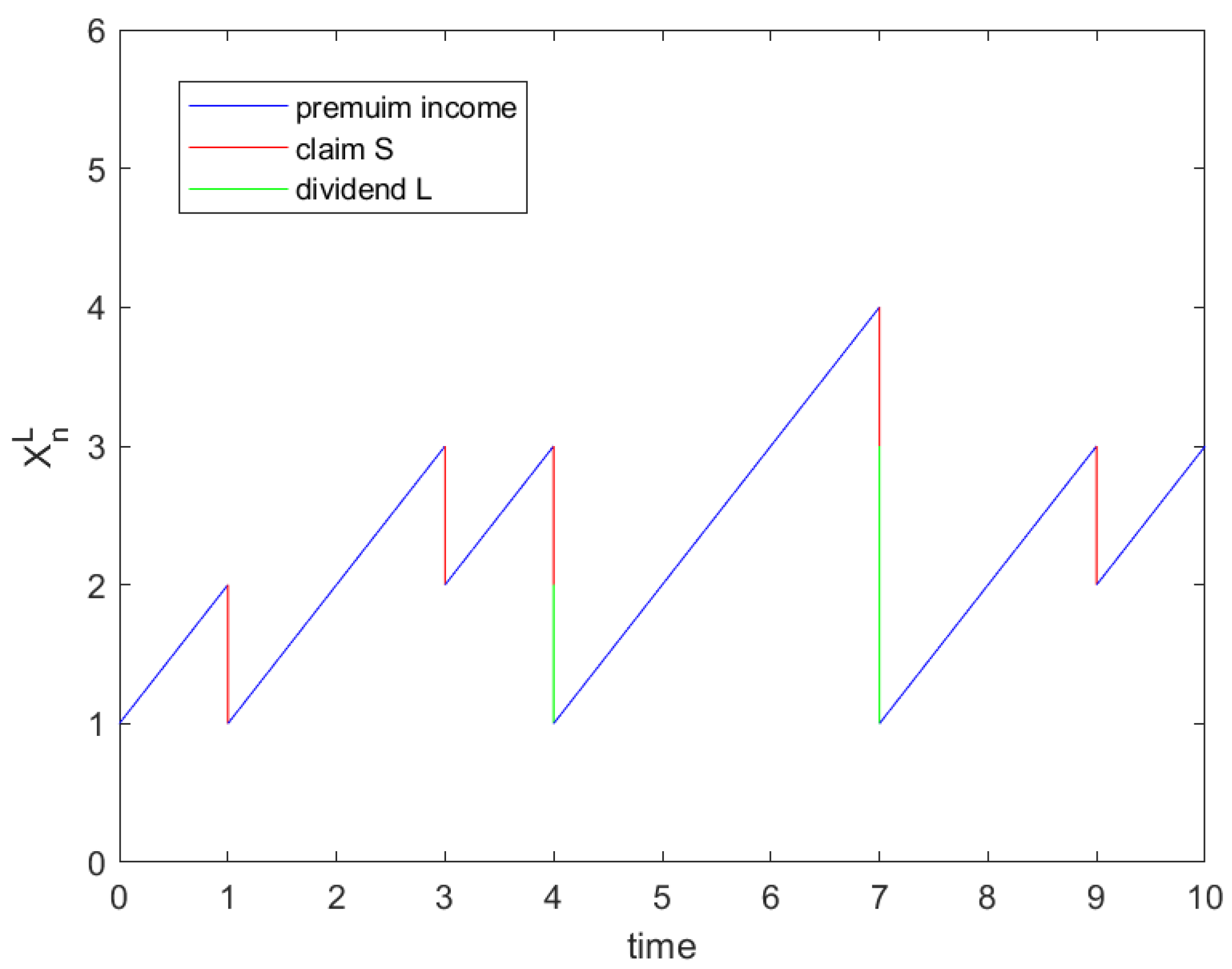
For better presentation, a diagram of one trajectory of the surplus process $X_n^L$ is shown in Figure 1.

Denote $\mathcal{K}$ the set of all admissible strategies and define the ruin time of the insurance company as follows:

$$\vartheta :=inf\{n\in {\mathbb{N}}_{+}|X_n^L<0\}.$$

For the initial wealth x, the initial interest rate $r_i$ (the initial discount rate $v_i$), and the given dividend policy ${\left\{\mathsf{\Delta }{L}_k\right\}}_{k=0}^{\infty }\in \mathcal{K}$, we define the following cumulative discounted dividend value with subsidies:

$$\begin{array}{c}\hfill J(x,i;L):=\mathbb{E}\left[\sum _{k=0}^{\vartheta }{u}_k(\mathsf{\Delta }{L}_k+\mathsf{\Lambda })\right],\end{array}$$

where $u_0=1,u_k:={\displaystyle \prod _{i=1}^k}{v}_i(k=1,2,\cdots$), $\mathsf{\Lambda }>0$ is a constant representing the subsidy of unit time. In [16], the authors considered the dividend optimization if a constant penalty is paid when the ruin occurs. Whereas, in our model, we consider that the shareholders can get a subsidy each unit time as long as the company is not ruined. We aim to find an optimal dividend strategy ${\left\{\mathsf{\Delta }{L}_k\right\}}_{k=0}^{\infty }\in \mathcal{K}$ to maximize $J(x,i;L)$. For notational simplicity we define the following value function:

$$V(x,i):=\underset{\mathsf{\Delta }L\in \mathcal{K}}{sup}J(x,i;L).$$

Apparently, the value function V is a m-dimensional vector-valued function. From the definition of the value function, we can easily obtain the following property.

Property 1. 

For any $x_1,x_2\in \mathbb{N}$ with $x_1>x_2$, it follows that

$$\begin{array}{c}\hfill V(x_1,i)-V(x_2,i)\ge x_1-x_2.\end{array}$$

Proof. 

For the initial wealth $x_1$ and initial interest rate $r_i$ (discount rate $v_i$), we choose a special strategy L such that $x_1-x_2$ is paid as dividend at the initial time and then follows the strategy $\tilde{L}$, where $\tilde{L}$ denotes any arbitrary strategy with initial data $(x_2,i)$. According to the definition of admissibility of dividend strategy, the lump dividend $x_1-x_2$ is allowed. Then, we can see that

$$V(x_1,i)\ge J(x_1,i;L)=J(x_2,i;\tilde{L})+x_1-x_2.$$

Since $\tilde{L}$ is arbitrary, we have $V(x_1,i)-V(x_2,i)\ge x_1-x_2.$ One can also find the similar idea which was used in other relevant references, for example, the proposition 2.2 of [18]. □

Now we show some preliminaries about the Banach fixed-point theorem which we will use in following paragraphs. We first show the definition of fixed point.

Definition 1. 

Let E be a metric space. We call a point z in E a fixed point of the mapping $\mathbf{G}:E\to E$ if $\mathbf{G}\left(z\right)=z.$

Definition 2.

Let $(E,d)$ be a complete metric space. We call a mapping $\mathbf{G}:E\to E$ a contraction mapping on E if there exists a constant $c\in [0,1)$ such that

$$d(\mathbf{G}\left(z_1\right),\mathbf{G}\left(z_2\right))\le cd(z_1,z_2)$$

for all $z_1,z_2\in E.$

Now we are ready to present the Banach contraction principle.

Theorem 1

(The Banach Contraction Principle). Let E be a complete metric space and the mapping $\mathbf{G}:E\to E$ be a contraction. Then $\mathbf{G}:E\to E$ has only one fixed point.

We omit the proof here. The Banach fixed-point theorem guarantees the existence and uniqueness of the fixed point and provides a method to find the fixed point. For more details about the Banach fixed-point theorems and its applications, we refer the interested reader to [19,20].

3. The Dynamic Programming Principle

Before stating our theorems, we first define the following notations for simplicity. Denote $\mathcal{U}$ the set of all mappings from ${\mathbb{N}}^0\times \{1,2,\cdots ,m\}$ to ${\mathbb{R}}_{+}^m$. Given the function $g\in \mathcal{U}$, $\mathsf{\Delta }L\in \{0,1,2,\cdots ,x\}$, define the function

$$\begin{array}{c}\hfill \begin{array}{c}\hfill q(x,j;g,\mathsf{\Delta }L):=\varrho \sum _{k=1}^{x+\beta -\mathsf{\Delta }L}{f}_{k}g(x+\beta -\mathsf{\Delta }L-k,j)+(1-\varrho )g(x+\beta -\mathsf{\Delta }L,j).\end{array}\end{array}$$

Utilize the classical dynamic programming principle, the value function has the following property.

Theorem 2. 

For the initial wealth x and the initial interest rate $r_i$ (in other words, the initial discount rate $v_i$), the value function satisfies

$$\begin{array}{c}\hfill \begin{array}{c}\hfill V(x,i)=\underset{\mathsf{\Delta }L\in \{0,1,2,\dots ,x\}}{sup}\left(\mathsf{\Delta }L+\mathsf{\Lambda }+v_i\sum _{j=1}^m{\mathbb{P}}_{ij}q(x,j;V,\mathsf{\Delta }L)\right),x=0,1,2\cdots ,\infty ;i=1,2,\cdots ,m.\end{array}\end{array}$$

(1)

When the surplus is x and the interest rate is $r_i,$ the optimal dividend $\mathsf{\Delta }{L}^{*}$ is

$$\begin{array}{c}\hfill arg\underset{\mathsf{\Delta }L\in \{0,1,2,\dots ,x\}}{max}\left(\mathsf{\Delta }L+v_i\sum _{j=1}^m{\mathbb{P}}_{ij}q(x,j;V,\mathsf{\Delta }L)\right).\end{array}$$

Proof. 

The dynamic programming equation has been proved in a lot of references, for example, the excellent books [21,22], hence we omit the detailed proof here. □

For the sake of notational simplicity, we define the operator $\mathbf{G}:\mathcal{U}\to \mathcal{U}$ as follows:

$$\begin{array}{cc}\hfill & \mathbf{G}\left(\begin{array}{c}g(·,1)\\ g(·,2)\\ ⋮\\ g(·,m)\end{array}\right)\left(x\right):=\left(\begin{array}{c}\underset{\mathsf{\Delta }L\in \{0,1,2,\dots ,x\}}{sup}\left(\mathsf{\Delta }L+\mathsf{\Lambda }+v_1\sum _{j=1}^m{\mathbb{P}}_{1j}q(x,j;g,\mathsf{\Delta }L)\right)\\ \underset{\mathsf{\Delta }L\in \{0,1,2,\dots ,x\}}{sup}\left(\mathsf{\Delta }L+\mathsf{\Lambda }+v_2\sum _{j=1}^m{\mathbb{P}}_{2j}q(x,j;g,\mathsf{\Delta }L)\right)\\ ⋮\\ \underset{\mathsf{\Delta }L\in \{0,1,2,\dots ,x\}}{sup}\left(\mathsf{\Delta }L+\mathsf{\Lambda }+v_m\sum _{j=1}^m{\mathbb{P}}_{mj}q(x,j;g,\mathsf{\Delta }L)\right)\end{array}\right).\hfill \end{array}$$

It is easy to see that the dynamic programming Equation (1) can be rewritten as

$$\begin{array}{c}\hfill \left(\begin{array}{c}V(·,1)\\ V(·,2)\\ ⋮\\ V(·,m)\end{array}\right)\left(x\right)=\mathbf{G}\left(\begin{array}{c}V(·,1)\\ V(·,2)\\ ⋮\\ V(·,m)\end{array}\right)\left(x\right).\end{array}$$

(2)

Now we show that there exists a unique solution for Equation (2). To this end, we only need to show that the mapping $\mathbf{G}$ is a contraction mapping. Accordingly, we have the following theorem:

Theorem 3.

The Equation (1) has a unique solution.

Proof. 

For any function $g\in \mathcal{U}$, define the norm by

$$\begin{array}{c}\hfill \begin{array}{cc}\hfill & \parallel {\left(g(·,1),g(·,2),\cdots ,g(·,m)\right)}^{\mathbf{T}}\parallel \hfill \\ \hfill :=& \max \left\{\underset{x\in {\mathbb{N}}^0}{\sup }\left|g(x,1)\right|,\underset{x\in {\mathbb{N}}^0}{\sup }\left|g(x,2)\right|,\cdots ,\underset{x\in {\mathbb{N}}^0}{\sup }\left|g(x,m)\right|\right\},\hfill \end{array}\end{array}$$

where $A^{\mathbf{T}}$ denotes the transpose matrix of the matrix A.

For any functions $\widehat{g},\tilde{g}\in \mathcal{U}$, define the metric d on $\mathcal{U}$ by

$$\begin{array}{c}\hfill \begin{array}{cc}\hfill & d\left({\left(\widehat{g}(·,1),\widehat{g}(·,2),\cdots ,\widehat{g}(·,m)\right)}^{\mathbf{T}},{\left(\tilde{g}(·,1),\tilde{g}(·,2),\cdots ,\tilde{g}(·,m)\right)}^{\mathbf{T}}\right)\hfill \\ \hfill :=& ∥{\left(\widehat{g}(·,1)-\tilde{g}(·,1),\widehat{g}(·,2)-\tilde{g}(·,2),\cdots ,\widehat{g}(·,m)-\tilde{g}(·,m)\right)}^{\mathbf{T}}∥\hfill \\ \hfill =& max\left\{\underset{x\in {\mathbb{N}}^0}{sup}|(\widehat{g}-\tilde{g})(x,1)|,\underset{x\in {\mathbb{N}}^0}{sup}|(\widehat{g}-\tilde{g})(x,2)|,\cdots ,\underset{x\in {\mathbb{N}}^0}{sup}\left|(\widehat{g}-\tilde{g})(x,m)\right|\right\}.\hfill \end{array}\end{array}$$

Then $(\mathcal{U},d)$ is a complete metric space.

Assume that $\widehat{\xi },\tilde{\xi }\in \mathcal{U},$ then

$$\begin{array}{c}\hfill d(\mathbf{G}\widehat{\xi },\mathbf{G}\tilde{\xi })=\parallel \mathbf{G}\widehat{\xi }-\mathbf{G}\tilde{\xi }\parallel .\end{array}$$

(3)

Obviously, $\mathbf{G}\widehat{\xi }-\mathbf{G}\tilde{\xi }$ is a m-dimensional column vector, we first consider the first item of such column vector.

It is not hard to verify that

$$\begin{array}{c}\hfill \begin{array}{cc}\hfill & |\underset{\mathsf{\Delta }L\in \{0,1,2,\dots ,x\}}{sup}\left(\mathsf{\Delta }L+\mathsf{\Lambda }+v_1\sum _{j=1}^m{\mathbb{P}}_{1j}q(x,j;\widehat{\xi },\mathsf{\Delta }L)\right)\hfill \\ & -\underset{\mathsf{\Delta }L\in \{0,1,2,\dots ,x\}}{sup}\left(\mathsf{\Delta }L+\mathsf{\Lambda }+v_1\sum _{j=1}^m{\mathbb{P}}_{1j}q(x,j;\tilde{\xi },\mathsf{\Delta }L)\right)|\hfill \\ \hfill \le & \underset{\mathsf{\Delta }L\in \{0,1,2,\dots ,x\}}{sup}{v}_1\sum _{j=1}^m{\mathbb{P}}_{1j}\left(\varrho \sum _{k=1}^{x+\beta -\mathsf{\Delta }L}{f}_k\underset{x\in {\mathbb{N}}^0}{sup}\left\{\right|\widehat{\xi }(·,j)-\tilde{\xi }(·,j)\left|\right\}+(1-\varrho )\underset{x\in {\mathbb{N}}^0}{sup}\left\{\right|\widehat{\xi }(·,j)-\tilde{\xi }(·,j)\left|\right\}\right)\hfill \\ \hfill \le & v_1\sum _{j=1}^m{\mathbb{P}}_{1j}\underset{x\in {\mathbb{N}}^0}{sup}\left\{\right|\widehat{\xi }(·,j)-\tilde{\xi }(·,j)\left|\right\}\hfill \\ \hfill \le & v_1\parallel \widehat{\xi }-\tilde{\xi }\parallel .\hfill \end{array}\end{array}$$

(4)

Similarly, we can show that for each $i\in \{2,\cdots ,m\},$ the i-th item of the vector $\mathbf{G}\widehat{\xi }-\mathbf{G}\tilde{\xi }$ satisfies

$$\begin{array}{c}\hfill \begin{array}{cc}\hfill & |\underset{\mathsf{\Delta }L\in \{0,1,2,\dots ,x\}}{sup}\left(\mathsf{\Delta }L+\mathsf{\Lambda }+v_i\sum _{j=1}^m{\mathbb{P}}_{ij}q(x,j;\widehat{\xi },\mathsf{\Delta }L)\right)\hfill \\ \hfill & -\underset{\mathsf{\Delta }L\in \{0,1,2,\dots ,x\}}{sup}\left(\mathsf{\Delta }L+\mathsf{\Lambda }+v_i\sum _{j=1}^m{\mathbb{P}}_{ij}q(x,j;\tilde{\xi },\mathsf{\Delta }L)\right)|\hfill \\ \hfill \le & \underset{\mathsf{\Delta }L\in \{0,1,2,\dots ,x\}}{sup}{v}_i\sum _{j=1}^m{\mathbb{P}}_{ij}\left(\varrho \sum _{k=1}^{x+\beta -\mathsf{\Delta }L}{f}_k\underset{x\in {\mathbb{N}}^0}{sup}\left\{\right|\widehat{\xi }(·,j)-\tilde{\xi }(·,j)\left|\right\}+(1-\varrho )\underset{x\in {\mathbb{N}}^0}{sup}\left\{\right|\widehat{\xi }(·,j)-\tilde{\xi }(·,j)\left|\right\}\right)\hfill \\ \hfill \le & v_i\sum _{j=1}^m{\mathbb{P}}_{ij}\underset{x\in {\mathbb{N}}^0}{sup}\left\{\right|\widehat{\xi }(·,j)-\tilde{\xi }(·,j)\left|\right\}\hfill \\ \hfill \le & v_i\parallel \widehat{\xi }-\tilde{\xi }\parallel .\hfill \end{array}\end{array}$$

(5)

Eventually, substituting the inequalities (4) and (5) into (3), we have

$$d(\mathbf{G}\widehat{\xi },\mathbf{G}\tilde{\xi })\le \tilde{v}\parallel \widehat{\xi }-\tilde{\xi }\parallel ,$$

where $\tilde{v}=max\{v_1,v_2,\cdots ,v_m\}<1$. Until now, we show that the mapping $\mathbf{G}:\mathcal{U}\to \mathcal{U}$ is a contraction mapping. Therefore, by using Banach contraction mapping principle, there exists a unique solution to the Equation (2) as well as the Equation (1). □

4. Algorithm

In this section, based on the proof of the uniqueness, we show an algorithm to solve the value function via Banach contraction mapping principle which is similar to the Bellman’s recursive algorithm used in [14].

(i)

We start from any real-valued function $W_0$. Choose $W_{old}(·,j)=W_0(·,j)(j=1,2,\cdots ,m)$ on ${\mathbb{N}}^0$ and define the new function $W_{new}(·,j)(j=1,2,\cdots ,m)$ by

$$\begin{array}{c}\hfill \left.\begin{array}{c}{W}_{new}(·,1)\\ W_{new}(·,2)\\ ⋮\\ W_{new}(·,m)\end{array}\right)\left(x\right):=\mathbf{G}\left(\begin{array}{c}{W}_{old}(·,1)\\ W_{old}(·,2)\\ ⋮\\ W_{old}(·,m)\end{array}\right)\left(x\right).\end{array}$$

(ii)

After calculating $W_{new}$, we choose $W_{old}:=W_{new}$ again and iterate the sequences $W_{old}$ and $W_{new}$ until both $W_{new}$ and $W_{old}$ converge.

Since the value function $V{(·,j)}_{j=1}^m$ is a fixed point of the contraction mapping $\mathbf{G}$, we can see that the value function

$$\begin{array}{c}\hfill V=\underset{n\to \infty }{lim}{\mathbf{G}}^n{W}_0.\end{array}$$

Consequently, as long as we choose n large enough, ${\mathbf{G}}^n{W}_0$ can be seen as a numerical solution of the value function $V{(·,j)}_{j=1}^m$.

Put $W_{n+1}=\mathbf{G}{W}_n$. On account of

$$\parallel W_{n+1}-W_n\parallel =\parallel \mathbf{G}{W}_n-\mathbf{G}{W}_{n-1}\parallel \le \tilde{v}\parallel W_n-W_{n-1}\parallel ,n=1,2,\cdots ,$$

we get that

$$\begin{array}{c}\hfill \parallel W_{n+1}-W_n\parallel \le \tilde{v}\parallel W_n-W_{n-1}\parallel \le \cdots {\tilde{v}}^n\parallel W_1-W_0\parallel .\end{array}$$

(6)

For any two positive integer $m,n$ with $m>n,$ it holds that

$$\begin{array}{c}\hfill \parallel W_m-W_n\parallel \le \parallel W_m-W_{m-1}\parallel +\parallel W_{m-1}-W_{m-2}\parallel +\cdots +\parallel W_{n+1}-W_n\parallel .\end{array}$$

(7)

Substituting (6) into (7) gives

$$\begin{array}{c}\hfill \parallel W_m-W_n\parallel \le ({\tilde{v}}^{m-1}+{\tilde{v}}^{m-2}+\cdots +{\tilde{v}}^n)\parallel W_1-W_0\parallel .\end{array}$$

(8)

Since the optimal value function $V={lim}_{m\to \infty }{W}_m$, letting $m\to \infty$ in (8) shows that the error estimation can be calculated as

$$\parallel V-W_n\parallel \le \frac{{\tilde{v}}^n}{1-\tilde{v}}\parallel W_1-W_0\parallel .$$

In the meanwhile, when the current surplus is x and the current interest rate is $r_i$, the optimal policy is

$$\begin{array}{c}\hfill arg\underset{\mathsf{\Delta }L\in \{0,1,2,\dots ,x\}}{max}\left(\mathsf{\Delta }L+v_i\sum _{j=1}^m{\mathbb{P}}_{ij}q(x,j;V,\mathsf{\Delta }L)\right).\end{array}$$

Remark 1.

In the real financial market, the dividend is paid with taxes (including fixed and proportional transaction costs). For example, Ref. [23] considered the optimal dividend problem considering fixed and proportional transaction costs and the equity issuance. In our model, if we consider the fixed and proportional transaction costs each time the dividend is paid, then the corresponding cumulative discounted dividend with the consideration of ruin time is defined as

$$\begin{array}{c}\hfill J(x,i):=\mathbb{E}\left[\sum _{k=0}^{\vartheta }{u}_k((\mu \mathsf{\Delta }{L}_k-\gamma ){\mathbf{1}}_{\{\mathsf{\Delta }{L}_k\ne 0\}}+\mathsf{\Lambda })\right],\end{array}$$

where ${\mathbf{1}}_A$ denotes the indicator function of the event $A,$ the constant $0<\mu <1$ represents the proportion of transaction fee and the constant $\gamma >0$ denotes the fixed transaction fee. Then the dynamic programming principle can be rewritten as

$$\begin{array}{c}\hfill \begin{array}{cc}\hfill & V(x,i)\hfill \\ \hfill =& \underset{\mathsf{\Delta }L\in \{0,1,2,\dots ,x\}}{sup}((\mu \mathsf{\Delta }L-\gamma ){\mathbf{1}}_{\{\mathsf{\Delta }L\ne 0\}}+\mathsf{\Lambda }\hfill \\ \hfill & +v_i\sum _{j=1}^m{\mathbb{P}}_{ij}\left(\varrho \sum _{k=1}^{x+\beta -\mathsf{\Delta }L}{f}_{k}V(x+\beta -\mathsf{\Delta }L-k,j)+(1-\varrho )V(x+\beta -\mathsf{\Delta }L,j)\right)).\hfill \end{array}\end{array}$$

The optimal policy $\mathsf{\Delta }{L}^{*}$ is calculated as

$$\begin{array}{cc}\hfill & arg\underset{\mathsf{\Delta }L\in \{0,1,2,\dots ,x\}}{sup}((\mu \mathsf{\Delta }L-\gamma ){\mathbf{1}}_{\{\mathsf{\Delta }L\ne 0\}}\hfill \\ \hfill & +v_i\sum _{j=1}^m{\mathbb{P}}_{ij}\left(\varrho \sum _{k=1}^{x+\beta -\mathsf{\Delta }L}{f}_{k}V(x+\beta -\mathsf{\Delta }L-k,j)+(1-\varrho )V(x+\beta -\mathsf{\Delta }L,j)\right)).\hfill \end{array}$$

All the above dynamic principles and algorithms can be rewritten similarly, thus, in this paper we only focus on the optimal dividend problem without transaction fees.

Remark 2.

The classical method of solving optimal dividend problem is to solve an explicit solution for the value function or analytically explore the structure of the optimal strategy, see, for example, Refs. [4,14]. In our paper, based on the fixed-point theory, we construct an algorithm to numerically calculate the optimal policy and the value function. Although there is no explicit expression for the value function, the advantages of using the fixed-point theory can be listed as: (1) There is no need to use the boundary condition. (2) The algorithm is easy to be used and constructed. (3) The complex theoretical calculation can be avoided.

5. Numerical Examples

Example 1. 

In this example, there are two different discount rates, $v_1=0.9$, $v_2=0.95$. The premium rate $\beta =10.$ The subsidy each unit time $\mathsf{\Lambda }=2$. The probability of claim occurs $\varrho =0.3$. The distribution of claim size follows

$$f_k=\mathbb{P}(S=k)=\frac{1}{25}{\left(\frac{24}{25}\right)}^k,k=1,2\cdots .$$

The transition matrix of the Markov chain is

$$\begin{array}{c}\hfill \mathbb{M}=\left(\begin{array}{cc}{\mathbb{P}}_{11}& {\mathbb{P}}_{12}\\ {\mathbb{P}}_{21}& {\mathbb{P}}_{22}\end{array}\right)=\left(\begin{array}{cc}\frac{1}{2}& \frac{1}{2}\\ \frac{1}{3}& \frac{2}{3}\end{array}\right).\end{array}$$

Now we show the numerical solution of the optimal policy and the value function under different discount rates.

Table 1. The optimal policy with discount rate $v_1=0.9$.

${\mathit{v}}_1=0.9$
x	0	1	2	3	4	5	6	7	8	9	10	11	12
$\mathsf{\Delta }{L}^{*}$	0	1	2	3	4	5	6	7	8	9	10	11	12

and

Table 2. The optimal policy with discount rate $v_1=0.95$.

${\mathit{v}}_2=0.95$
x	0	1	2	3	4	5	6	7	8	9	10	11	12
$\mathsf{\Delta }{L}^{*}$	0	0	0	0	0	1	2	3	4	5	6	7	8

show the optimal policy under the discount rate $v_1=0.9$, $v_2=0.95$, respectively. When the discount rate $v_1=0.9$, the dividend barrier is 0, which means that, all the surplus above value 0 will be paid as dividend. Compared with the discount rate 0.9, when the discount rate is 0.95, the dividend barrier is 4, which means that, all surplus above the value 4 will be paid as dividend. This phenomenon can be explained that if the discount rate is low, which means the interest rate is high, then the company manager will pay more cash to the shareholders. If the interest rate is low, then the company prefers to save money and waits until the interest rate is high.

Table 3. The value function with discount rate $0.9$.

${\mathit{v}}_1=0.9$
x	0	1	2	3	4	5	6	7	8	9	10	11
$V(x,1)$	33.35	34.35	35.35	36.35	37.35	38.35	39.35	40.35	41.35	42.35	43.35	44.35

and

Table 4. The value function with discount rate $0.95$.

${\mathit{v}}_2=0.95$
x	0	1	2	3	4	5	6	7	8	9	10	11
$V(x,2)$	35.34	36.35	37.36	38.3665	39.3675	40.36	41.36	42.36	43.36	44.36	45.36	46.36

show the value function with the discount rate $v_1=0.9$, $v_2=0.95$, respectively. When the optimal policy is not paying dividend, the increment of the value function is larger than 1. In economics, it can be explained that paying no dividend can bring more benefits when the interest rate is low.

Example 2. 

In this example, we consider that there are three different discount rates, $v_1=0.94$, $v_2=0.95$, $v_3=0.98$. The transition probability matrix

$$\begin{array}{c}\hfill \mathbb{M}=\left(\begin{array}{ccc}\frac{1}{2}& \frac{1}{4}& \frac{1}{4}\\ \frac{1}{6}& \frac{1}{2}& \frac{1}{3}\\ \frac{1}{3}& \frac{1}{3}& \frac{1}{3}\end{array}\right).\end{array}$$

The premium rate $\beta =10$. The probability of claim occurs ϱ is $0.3$ and the subsidy each unit time Λ is still 2. Assume that the claim amount distribution follows the uniform distribution with distribution function

$$f_k=\mathbb{P}(S=k)=\frac{1}{50},k=1,2,\cdots ,50.$$

Table 5. The optimal dividend policy with discount rate $v_1=0.93$.

${\mathit{v}}_1=0.93$
x	$\mathsf{\Delta }{\mathit{L}}^{*}$	x	$\mathsf{\Delta }{\mathit{L}}^{*}$	x	$\mathsf{\Delta }{\mathit{L}}^{*}$	x	$\mathsf{\Delta }{\mathit{L}}^{*}$	x	$\mathsf{\Delta }{\mathit{L}}^{*}$	x	$\mathsf{\Delta }{\mathit{L}}^{*}$	x	$\mathsf{\Delta }{\mathit{L}}^{*}$
0	0	7	7	14	14	21	21	28	28	35	0	42	2
1	1	8	8	15	15	22	22	29	29	36	0	43	3
2	2	9	9	16	16	23	23	30	0	37	0	44	4
3	3	10	10	17	17	24	24	31	0	38	0	45	5
4	4	11	11	18	18	25	25	32	0	39	0	46	6
5	5	12	12	19	19	26	26	33	0	40	0	47	7
6	6	13	13	20	20	27	27	34	0	41	1	48	8

,

Table 6. The optimal dividend policy with discount rate $v_2=0.96$.

${\mathit{v}}_2=0.96$
x	$\mathsf{\Delta }{\mathit{L}}^{*}$	x	$\mathsf{\Delta }{\mathit{L}}^{*}$	x	$\mathsf{\Delta }{\mathit{L}}^{*}$	x	$\mathsf{\Delta }{\mathit{L}}^{*}$	x	$\mathsf{\Delta }{\mathit{L}}^{*}$	x	$\mathsf{\Delta }{\mathit{L}}^{*}$	x	$\mathsf{\Delta }{\mathit{L}}^{*}$
0	0	7	7	14	14	21	0	28	0	35	0	42	2
1	1	8	8	15	15	22	0	29	0	36	0	43	3
2	2	9	9	16	16	23	0	30	0	37	0	44	4
3	3	10	10	17	17	24	0	31	0	38	0	45	5
4	4	11	11	18	18	25	0	32	0	39	0	46	6
5	5	12	12	19	19	26	0	33	0	40	0	47	7
6	6	13	13	20	0	27	0	34	0	41	1	48	8

and

Table 7. The optimal dividend policy with discount rate $v_3=0.95$.

${\mathit{v}}_3=0.95$
x	$\mathsf{\Delta }{L}^{*}$	x	$\mathsf{\Delta }{\mathit{L}}^{*}$	x	$\mathsf{\Delta }{\mathit{L}}^{*}$	x	$\mathsf{\Delta }{\mathit{L}}^{*}$	x	$\mathsf{\Delta }{\mathit{L}}^{*}$	x	$\mathsf{\Delta }{\mathit{L}}^{*}$	x	$\mathsf{\Delta }{\mathit{L}}^{*}$
0	0	7	7	14	14	21	21	28	0	35	0	42	2
1	1	8	8	15	15	22	22	29	0	36	0	43	3
2	2	9	9	16	16	23	23	30	0	37	0	44	4
3	3	10	10	17	17	24	0	31	0	38	0	45	5
4	4	11	11	18	18	25	0	32	0	39	0	46	6
5	5	12	12	19	19	26	0	33	0	40	0	47	7
6	6	13	13	20	20	27	0	34	0	41	1	48	8

list the optimal dividend policy under different discount rate $v_1=0.93$, $v_2=0.96$ and $v_3=0.95$, respectively. As we can see, when the discount factor is $0.93$, there are two dividend barriers, the first one is 0 and the second one is 41. For all $x\in \{0,1,\cdots ,29\}$, all surplus above value 0 will be paid as dividend. When $x\in \{30,31,\cdots ,40\}$, no dividend is paid. When $x\in \{41,42,\cdots \}$, all the surplus above the value 40 will be paid as dividend. The no-dividend region is $\{30,31,\cdots ,40\}$. This kind of policy is called the band strategy (i.e., there are more than 1 dividend barrier). When the discount rate is $0.96$, the no-dividend region is $\{20,21,\cdots ,40\}$. When the discount rate is $0.95$, the no-dividend region is $\{24,25,\cdots ,40\}$.

Table 8. The value function with discount rate $v_1=0.93$.

${\mathit{v}}_1=0.93$
x	$\mathit{V}(\mathit{x},\mathbf{1})$	x	$\mathit{V}(\mathit{x},\mathbf{1})$	x	$\mathit{V}(\mathit{x},\mathbf{1})$	x	$\mathit{V}(\mathit{x},\mathbf{1})$	x	$\mathit{V}(\mathit{x},\mathbf{1})$	x	$\mathit{V}(\mathit{x},\mathbf{1})$	x	$\mathit{V}(\mathit{x},\mathbf{1})$
0	31.05	7	38.05	14	45.05	21	52.05	28	59.05	35	66.42	42	73.91
1	32.05	8	39.05	15	46.05	22	53.05	29	60.05	36	67.51	43	74.91
2	33.05	9	40.05	16	47.05	23	54.05	30	61.07	37	68.60	44	75.91
3	34.05	10	41.05	17	48.05	24	55.05	31	62.13	38	69.70	45	76.91
4	35.05	11	42.05	18	49.05	25	56.05	32	63.19	39	70.80	46	77.91
5	36.05	12	43.05	19	50.05	26	57.05	33	64.27	40	71.91	47	78.91
6	37.05	13	44.05	20	51.05	27	58.05	34	65.34	41	72.91	48	79.91

,

Table 9. The value function with discount rate $v_2=0.96$.

${\mathit{v}}_2=0.96$
x	$\mathit{V}(\mathit{x},\mathbf{2})$	x	$\mathit{V}(\mathit{x},\mathbf{2})$	x	$\mathit{V}(\mathit{x},\mathbf{2})$	x	$\mathit{V}(\mathit{x},\mathbf{2})$	x	$\mathit{V}(\mathit{x},\mathbf{2})$	x	$\mathit{V}(\mathit{x},\mathbf{2})$	x	$\mathit{V}(\mathit{x},\mathbf{2})$
0	32.25	7	39.25	14	46.25	21	53.42	28	61.35	35	69.26	42	76.96
1	33.25	8	40.25	15	47.25	22	54.52	29	62.53	36	70.39	43	77.96
2	34.25	9	41.25	16	48.25	23	55.63	30	63.71	37	71.52	44	78.96
3	35.25	10	42.25	17	49.25	24	56.76	31	64.81	38	72.66	45	79.96
4	36.25	11	43.25	18	50.25	25	57.89	32	65.92	39	73.81	46	80.96
5	37.25	12	44.25	19	51.25	26	59.03	33	67.03	40	74.96	47	81.96
6	38.25	13	45.25	20	52.32	27	60.19	34	68.14	41	75.96	48	82.96

and

Table 10. The value function with discount rate $v_3=0.95$.

${\mathit{v}}_3=0.95$
x	$\mathit{V}(\mathit{x},\mathbf{3})$	x	$\mathit{V}(\mathit{x},\mathbf{3})$	x	$\mathit{V}(\mathit{x},\mathbf{3})$	x	$\mathit{V}(\mathit{x},\mathbf{3})$	x	$\mathit{V}(\mathit{x},\mathbf{3})$	x	$\mathit{V}(\mathit{x},\mathbf{3})$	x	$\mathit{V}(\mathit{x},\mathbf{3})$
0	31.79	7	38.79	14	45.79	21	52.79	28	60.34	35	68.14	42	75.76
1	32.79	8	39.79	15	46.79	22	53.79	29	61.50	36	69.26	43	76.76
2	33.79	9	40.79	16	47.79	23	54.79	30	62.67	37	70.38	44	77.76
3	34.79	10	41.79	17	48.79	24	55.82	31	63.75	38	71.50	45	78.76
4	35.79	11	42.79	18	49.79	25	56.94	32	64.84	39	72.63	46	79.76
5	36.79	12	43.79	19	50.79	26	58.07	33	65.93	40	73.76	47	80.76
6	37.79	13	44.79	20	51.79	27	59.20	34	67.04	41	74.76	48	81.76

list the value function under different interest rates $v_1=0.93$, $v_2=0.96$ and $v_3=0.95$, respectively. We can see that when the optimal policy is not paying dividend, the increment of the value function is larger than 1. When the optimal policy is to pay the dividend, the increment of the dividend is exactly 1. Such numerical phenomenon also verifies the Property 1 in Section 2.

6. Conclusions

In this paper, the optimal dividend optimization with subsidies under different interest rates are explored. When the claims follow the geometric distribution, the optimal dividend policy is a barrier strategy while the barrier is decided by the current interest rate. When the claims follow the uniform distribution, then the optimal dividend policy is of multiple barrier type, i.e., the band type. We conclude that the optimal dividend policy will be different under different claim distributions.

References

1. De Finetti, B. Su un’impostazione alternativa della teoria collettiva del rischio. Trans. XVth Int. Congr. Actuar. 1957, 2, 433–443. [Google Scholar]
2. Jeanblanc-Picqué, M.; Shiryaev, A.N. Optimization of the flow of dividends. Usp. Mat. Nauk. 1995, 50, 25–46. [Google Scholar] [CrossRef]
3. Asmussen, S.; Taksar, M. Controlled diffusion models for optimal dividend pay-out. Insur. Math. Econ. 1997, 20, 1–15. [Google Scholar] [CrossRef]
4. Gerber, H.U.; Shiu, E.S. On optimal dividend strategies in the compound Poisson model. N. Am. Actuar. J. 2006, 10, 76–93. [Google Scholar] [CrossRef]
5. Bai, L.; Ma, J.; Xing, X. Optimal dividend and investment problems under Sparre Andersen model. Ann. Appl. Probab. 2017, 27, 3588–3632. [Google Scholar] [CrossRef]
6. Asmussen, S.; Højgaard, B.; Taksar, M. Optimal risk control and dividend distribution policies. Example of excess-of loss reinsurance for an insurance corporation. Financ. Stoch. 2000, 4, 299–324. [Google Scholar] [CrossRef]
7. Albrecher, H.; Hartinger, J. On the non-optimality of horizontal barrier strategies in the Sparre Andersen model. Hermis: Int. J. Comput. Math. Appl. 2006, 7, 109–122. [Google Scholar]
8. Albrecher, H.; Thonhauser, S. Optimal dividend strategies for a risk process under force of interest. Insur. Math. Econ. 2008, 43, 134–149. [Google Scholar] [CrossRef]
9. Albrecher, H.; Thonhauser, S. Optimality results for dividend problems in insurance. Racsam. Rev. R. Acad. A. 2009, 103, 295–320. [Google Scholar] [CrossRef]
10. Chen, S.; Li, Z.; Zeng, Y. Optimal dividend strategy for a general diffusion process with time-inconsistent preferences and ruin penalty. SIAM J. Financ. Math. 2018, 9, 274–314. [Google Scholar] [CrossRef]
11. Hernandez, C.; Junca, M.; Moreno-Franco, H. A time of ruin constrained optimal dividend problem for spectrally one-sided Lévy processes. Insur. Math. Econ. 2018, 79, 57–68. [Google Scholar] [CrossRef]
12. Akyildirim, E.; Güney, I.E.; Rochet, J.C.; Soner, H.M. Optimal dividend policy with random interest rates. J. Math. Econ. 2014, 51, 93–101. [Google Scholar] [CrossRef]
13. Eisenberg, J. Optimal dividends under a stochastic interest rate. Insur. Math. Econ. 2015, 65, 259–266. [Google Scholar] [CrossRef]
14. Gerber, H.U.; Shiu, E.S.; Yang, H. An elementary approach to discrete models of dividend strategies. Insur. Math. Econ. 2010, 46, 109–116. [Google Scholar] [CrossRef]
15. Tan, J.; Yang, X. Optimal dividend strategy in compound binomial model with bounded dividend rates. Acta Math. Appl. Sin. Engl. Ser. 2014, 30, 859–870. [Google Scholar] [CrossRef]
16. Tan, J.; Li, C.; Li, Z.; Yang, X.; Zhang, B. Optimal dividend strategies in a delayed claim risk model with dividends discounted by stochastic interest rates. Math. Meth. Oper. Res. 2015, 82, 61–83. [Google Scholar] [CrossRef]
17. Thonhauser, S.; Albrecher, H. Dividend maximization under consideration of the time value of ruin. Insur. Math. Econ. 2007, 41, 163–184. [Google Scholar] [CrossRef]
18. Azcue, P.; Muler, N. Optimal reinsurance and dividend distribution policies in the Cramér-Lundberg model. Math. Finance 2005, 15, 261–308. [Google Scholar] [CrossRef]
19. Agarwal, R.P.; Meehan, M.; O’regan, D. Fixed Point Theory and Applications; Cambridge University Press: Cambridge, UK, 2001. [Google Scholar]
20. Royden, H.L.; Fitzpatrick, P. Real Analysis; Macmillan: New York, NY, USA, 1988. [Google Scholar]
21. Ross, S.M. Introduction to Stochastic Dynamic Programming; Academic Press: Cambridge, MA, USA, 2014. [Google Scholar]
22. Fleming, W.H.; Soner, H.M. Controlled Markov Processes and Viscosity Solutions; Springer: New York, NY, USA, 2006. [Google Scholar]
23. He, L.; Liang, Z. Optimal financing and dividend control of the insurance company with fixed and proportional transaction costs. Insur. Math. Econ. 2009, 44, 88–94. [Google Scholar] [CrossRef]
Figure 1. One trajectory of the surplus process X n L .
Mathematics 11 00902 g001