A Novel Hybrid Deep Neural Network for Predicting Athlete Performance Using Dynamic Brain Waves

Abstract

The exploration of the performance of elite athletes by cognitive neuroscience as a research method has become an emerging field of study in recent years. In the research of cognitive abilities and athletic performance of elite athletes, the tasks of an experiment are usually performed by athletics task of closed skills rather than open skills. Thus, little has been conducted to explore the cognitive abilities and athletic performance of elite athletes with open skills. This study is novel as it attempts at predicting how table tennis athletes perform by collecting their dynamic brain waves when executing specific plays of table tennis, and then putting the data of dynamic brain waves to deep neural network algorithms. The method of this study begins with the collection of data on the dynamic brain waves of table tennis athletes and then converts the time domain data into frequency domain data before improving the accuracy of categorization using a hybrid convolutional neural networks (CNN) framework of deep learning. The findings hereof were that the algorithm of hybrid deep neural networks proposed herein was able to predict the sports performance of athletes from their dynamic brain waves with an accuracy up to 96.70%. This study contributes to the literature in cognitive neuroscience on dynamic brain waves in open skills and creates a novel hybrid deep CNN classification model for identifying dynamic brain waves associated with good elite sports performance.

1. Introduction

In athletes who have undergone training in pursuit of higher, faster, and stronger, their cognitive ability of the brain becomes different significantly. Elite athletes outperform average athletes or non-athletes cognitively, which shows that cognitive performance is crucial to sports performance [1,2]. The exploration of elite sports performance by the research method of cognitive neuroscience has become an emerging field of research in recent years. To understand the brain mechanism of cognitive ability behind sports performance, researchers can make an observation on the status of brain activities by means of neuroimaging technology, which include electroencephalography (EEG), magnetoencephalography (MEG), functional magnetic resonance imaging (fMRI), positron emission tomography (PET), functional near-infrared spectroscopy (fNIRS), and others [3,4,5,6]. EEG is characterized by high temporal resolution, is handy to use and non-invasive, and has been widely used in examining the status of brain activities [7]. The status of brain activities can reflect mental statuses such as cognitive ability, concentration, and emotion [8].

It is demonstrated by increasing evidence that elite athletes have better cognitive performance than average athletes or non-athletes, where cognitive abilities include perception, attention, memory, decision, and expectation, among others. An examination by analysis of variance (ANOVA) of Theta (4–8 Hz) waves at the middle frontal lobe on successful and failed penalty throws collected two seconds prior to the throw by basketball athletes in a task of penalty throw discovered that stable Theta waves at middle frontal lobe before the execution could enable better performance, the power of Theta waves at middle frontal lobe being an indicator of attention [9]. Both badminton athletes and non-athletes were put to non-delayed and delayed matching-to-sample tests, and a Pearson correlation analysis discovered that the synchronization of higher Theta waves (4–7 Hz) showed higher attention, while dropping out of synchronization of higher Beta waves (15–30 Hz) showed faster cognitive treatment [10]. An analysis of brain waves collected two seconds prior to throwing darts by both dart experts and novices by the method of ANOVA revealed that the experts’ sensorimotor rhythm, SMR, had higher power than the novices, where SMR is exactly the Beta waves (12–15 Hz) at the sensing area of the brain on sports. That reflected that regarding adaptive regulation by cognitive-motor treatment in the preparatory stage, the experts were seen with less interference than novices with proprioception and information, which was consistent with the Psychomotor efficiency hypothesis [11]. An ANOVA analysis of the EEG data that were sampled from skilled air-pistol experts for 3 s before shotting revealed that well performing experts had the last-second brain waves before shooting with higher SMR power, which indicated higher SMR powers reduced interference with sensorimotor processing and in turn increased the processing efficiency [12]. The reaction time and N200 (negative wave at about post-event 200 ms) and P300 (positive wave at about post-event 300 ms) amplitudes of brain waves and latency of both table tennis athletes and non-athletes on a masked go/no-go task were analyzed, which showed that table tennis athletes exhibited better cognitive control than average people [13]. At-rest brain waves of baseball athletes were collected before batting practice for determining the mean power of the various frequencies and an inverse relation was found between the power of pre-practice prefrontal lobe Beta wave and the batting performance, that is, when the power of frontal lobe Beta wave was lower, the batting performance was better [14]. Where the brain waves of elite golfers from two seconds to zero second before putting were analyzed with ANOVA, there was a coherence between elite golfers during putting and amateur golfer in terms of lower alpha 2 power at the right temporal lobe and lower alpha 2 at the front temporal lobe-left temporal lobe and front temporal lobe-right temporal lobe; it is thus clear that elite golfers committed more attention than amateurs, in addition to less cognitive-motor interference [15].

However, currently, the research focuses on the observation of athletes’ performance in cognitive ability by using videos of cognitive tasks conducted at labs [10,13] or at static sports tasks of closed skills [9,11,12] instead of dynamic sports tasks of open skills. In a sport of closed skills, where the environment tends to be unchanged, the motions of athletes are more regular and repetitive, e.g., dart throwing, shooting, and golf putting, which are relatively static sports. In a sport of open skills, as the environment changes significantly, athletes have to make adjustments or continue moving according to their opponents or the environment, e.g., football, tennis, and table tennis, which are more dynamic sports.

In addition, currently, the research with static sports tasks involves the observation of the data of the static brain waves that are collected within a few seconds from the preparation before a sports performance to the completion of an action, and the analysis of variance by conventional statistic methods. On the other hand, given larger amounts of data on dynamic brain waves, researchers can employ methods of machine learning or deep learning to conduct training and make predictions. Machine learning is a branch of artificial intelligence and can, through learning on the training dataset, automatically identify implicit rules in data, as well as make predictions based on those rules. Deep learning, a subdomain of machine learning, differs in that it is an algorithm of artificial neural networks with multi-layers, and can automatically extract features [16,17]. For deep learning, computer vision (CV) tasks are primarily subject to the framework of convolutional neural networks (CNN) [18], and natural language processing (NLP) tasks are primarily subject to the framework of long short-term memory (LSTM) or Transformer [19]. Deep learning has been successfully applied to many EEG tasks, including motor imagery, mental load, emotion recognition, event-related potential, etc. [20,21,22]. Part of the research mentioned above compared the hybrid architecture that was proposed from deep learning and those based on standard architecture, and the findings indicated that the hybrid architecture was superior to standard architecture, including CNN combined with LSTM and CNN combined with Transformer [23,24,25,26,27].

With the above summarized, currently, the research on dynamic brain waves of elite athletes in dynamic sports is still wanted. Dynamic brain waves mean the brain waves generated by people during dynamic sports. Dynamic sports are whole-body movements, rather than partial-body movements. Open-skill dynamic sports can obtain brain waves during long-term movements, instead of closed-skill static sports, which only have brain waves in a few seconds. Therefore, this study is very important to study the dynamic brain wave characteristics of sports performance. Among the sports of open skills, because table tennis requires less space than football, tennis, basketball, or boxing, which allows the use of a portable multi-channel brain–computer interface, BCI, at experiments and for collecting signals of dynamic brain waves. Hence, this study aims to build a novel deep learning categorization model of hybrid architecture that can predict sports performance by using the dynamic brain waves of table tennis athletes in executing specific table tennis tasks and to identify the major brain wave features that are related to sports performance.

The contributions of this study are:

• Extending the literature regarding dynamic brain waves of cognitive neuroscience on open skills;
• Creating a new categorization model for deep learning for distinguishing the brain waves of elite table tennis athletes when performing well;
• Identifying the key features of brain waves on elite table tennis athletes when performing well.

This paper comprises four sections: Section 1 presents the current introduction; Section 2 outlines how the signals of dynamic brain waves of table tennis athletes are collected, and the methods of data pre-processing and data analysis; Section 3 presents the results of sports performance categorization, comparisons and discussions; and Section 4 gives final conclusions and recommendations for future research.

2. Materials and Methods

The experiment process of this study as shown in Figure 1 comprises three stages. The first is data collection; the second is data pre-processing; and the third is data analysis. The stage of data collection uses BCI to collect the dataset of dynamic brain waves from table tennis athletes in executing specific table tennis tasks. The stage of data pre-processing rules out unnecessary signals and converts data from the time domain into the frequency domain. The stage of data analysis uses a hybrid deep learning algorithm in feature analysis before constructing an optimal categorization model for predicting sports performance, and finally identifying the most critical brain wave features in the model.

2.1. Data Collection

2.1.1. Participants

To begin with, this study passed the review by the First Human Research Ethics Review Board affiliated with the College of Medicine, National Cheng Kung University (A-ER-108-041). This study recruited table tennis players from the National Taiwan University of Sport. The participants were 16 table tennis players (Age = 20.63 ± 0.86, Male = 8, Female = 8). Prior to the onset of experiment, we explained to the participants about the details of the experiment process and had every one of them sign on the descriptions of human research and written consent.

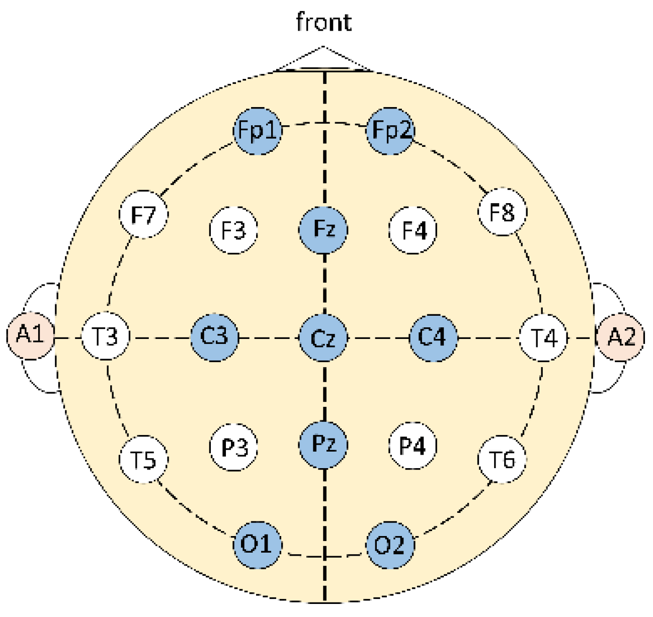
2.1.2. Tools

• EEG device;
• The EEG device is a commercially available porTable 40-lead neuroimaging potential recording system, including a dry electrode cap, a power amplifier, a computer cable, and a set of data acquisition software Curry 8. When in use, the electrode cap is connected to the power amplifier, and then connected to the laptop. The current EEG status is displayed through the data acquisition software in the laptop, and the EEG can be saved as a file.
• This EEG device has dedicated data collection software, and it is not possible to make software to read real-time data. Unlike some EEG devices that use an open architecture, they can read real-time data by themselves [28].
• Software.
• The data analysis is performed in the Google Colab environment, and the software uses Python 3.8.10, Tensorflow 2.9.2, and Keras 2.9.0 to design the models and execute them.

2.1.3. Table Tennis Test

In an indoor table tennis training court, the subjects wear a porTable 40-channel BCI, with its leads attached to the scalp, behind the ears, and on the face at the electrode positions with the help of conductive glue. For electrode positions, the International 10–20 system [29,30] is used, as Figure 2 shows. Records are taken at 9 electrode positions on the head, namely, Fp1 (frontal polar right), Fp2 (frontal polar left), Fz (midline frontal), C3 (central left), C4 (central right), Cz (midline central), Pz (midline parietal), O1 (occipital left), and O2 (occipital right). Additionally, records are taken at the forehead GND position as a ground electrode, A1 (mastoid bone by the left ear) and A2 (mastoid bone by the right ear) as reference points, in addition to VEOU (vertical electrooculogram upper), VEOL (vertical electrooculogram lower), HEOL (horizontally on the outside of the left eye) and HEOR (horizontally on the outside of the right eye) for electrooculography (EOG) activity to rule out the wave-interfering eye motion. The electric resistance at every electrode is below 5 Ω, and the intensity of electric brain waves is μV signals, with a sampling rate of 1024 Hz. Electric potential changes at the electrode positions are all collected throughout the experiment process.

In the beginning, the 60 s brain waves of each participant at closed eye and relaxed rest are taken; then, they are put to specific table tennis tests, which are accurate and fast reacting tests for them. Each participant undergoes 4 specific tests. (1) Hit the slowballs 50 times on the front of the table. (2) Hit the slowballs 50 times on the side of the table. (3) Hit the fastballs 20 times on the front of the table. (4) Hit the fastballs 20 times on the side of the table. 30 slowballs per minute and 50 fastballs per minute. There is a white rectangular area (30 cm × 25 cm) on the left side, in the middle, and on the right side of the end section of the table. A participant must hit a tossed ball to land in a designated white area to score. Another 60 s brain wave will be recorded at closed-eye relaxed rest after the 4 tests are completed.

2.2. Data Pre-Processing

2.2.1. Filter

Filters are for ruling out undesired noises and acquiring signals of specific frequencies. There is the low pass filter, high pass filter, band pass filter, and band reject filter. The Butterworth filter is a filter that has a steadier characteristic than other filters [31], thus a Butterworth low pass filter is used in this study to acquire the band of 0–70 Hz. See Equation (1)

$$G_n\left(\omega \right)=\left|H_n\left(j\omega \right)\right|=\frac{1}{\sqrt{1+{\left(\frac{\omega }{{\omega }_c}\right)}^{2n}}}$$

(1)

where $H$ is the transfer function, $n$ represents the order of the filter, $j$ is the Imaginary unit, $\omega$ represents the angular frequency, and ${\omega }_c$ is the cutoff frequency.

2.2.2. Feature Transform

Signals are analyzed chiefly by time domain and frequency domain. With phases being ignored, the former is the changes of signal amplitudes in terms of time and the latter is the changes of signal amplitudes in terms of frequency. Since many studies in the past used frequency-domain signals as input features, this method is also adopted in this study. Fourier transform can dissolve a signal into sine waves of different amplitudes and frequencies, converting a signal of the time domain into one of frequency. By means of fast Fourier transform (FFT), this study landed the power spectral density (PSD) of each brain wave. See Equation (2):

$$X_k=\sum _{j=0}^{n-1}{x}_j{e}^{-2\pi ikj/n},k=0,1,\dots n-1$$

(2)

where $X$ represents the discrete frequency signal, $x$ is the discrete time signal, and n represents the number of samples.

In the dataset of this study, there were 9 electrode positions, which are Fp1, Fp2, Fz, C3, Cz, C4, Pz, O1, and O2. Each electrode data is processed by FFT (the length of FFT length is 1024) to generate 8 brain waves data, which are Delta 0–4 Hz, Theta 4–8 Hz, Low Alpha 8–10 Hz, High Alpha 10–13 Hz, Low Beta 13–20 Hz, High Beta 20–30 Hz, Low Gamma 30–46 Hz and High Gamma 46–70 Hz. As such, there are 72 features.

2.2.3. Data Labeling

Brain wave data are marked into two categories, which are good and poor. The sports performance in a specific table tennis test with a score that exceeds the average value is a good one or a poor one with a score below the average.

2.2.4. Convert 1D Array to 2D Array

A record that was originally 1D is transformed into 2D data as input to the neural network, as Figure 3 shows:

2.3. Data Analysis

2.3.1. Hybrid Architecture

The hybrid architecture for the deep learning model herein is a two-level categorization task to be executed with the data of dynamic brain waves of table tennis athletes to distinguish between good and poor sports performance. Its main framework, as Figure 4 shows, where an input undergoes a first convolution layer and a first block, then a second convolution layer for pooling, a second block, and a third convolution layer, before being categorized by a fully connected layer, global average pooling, and fully connected layer, where a block is a combination of different modules. There are currently three main neural network frameworks for CV tasks: CNN, Transformer, and multi-layer perceptron (MLP) [32]. in this study, the MBConv block of Efficientnetv2 [33], the Transformer block of ViT [34], and the Mixer block of MLP-Mixer [35] are used, where the different blocks are combined in parallel. A total of 7 combinations were adopted in this study to identify the optimal models, as

Table 1. 7 hybrid models of different combinations in this study.

Model	Blocks
CNet	MBConv
TNet	Transformer
MNet	Mixer
CTNet	MBConv, Transformer
CMNet	MBConv, Mixer
TMNet	Transformer, Mixer
CTMNet	MBConv, Transformer, Mixer

shows.

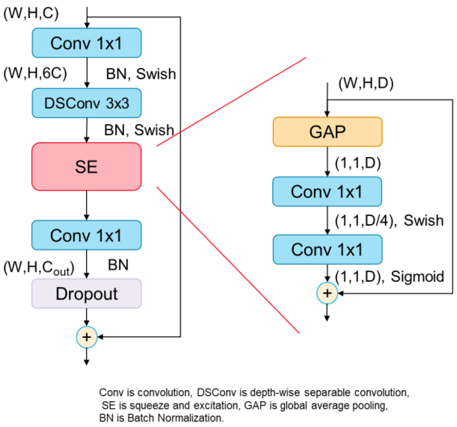
2.3.2. MBConv Block

MBConv is an inverted linear bottleneck layer of depth-wise separable convolutions, comprising depth-wise separable convolutions and squeeze and excitation (SE) module. The depth-wise separable convolutions mean the division of a normal 3 × 3 convolution into two convolutions, including the depth-wise convolution and the point-wise convolution. The depth-wise convolution is executed first, i.e., the 3 × 3 convolution is executed on each channel, before concatenation; then is followed by the point-wise convolution, which executes 1 × 1 convolution on each channel. This reduces a large number of parameters compared with a common 3 × 3 convolution while achieving the same effect, as Figure 5 shows.

MBConv block is composed as follows:

• Convolutional Layer;
• Equations for the convolutional layer are as Equations (3) and (4) shows.
• Forward:

$$z^l=a^{l-1}\ast W^l+b^l$$

(3)

$$a^l=f^l\left(z^l\right)$$

(4)

where $z^l$ is the result of the $l$th convolution, $a^{l-1}$ is the output of the $l-1$th layer, $\ast$ is the operation of convolution, $W^l$ is the weight for the $l$th layer, $b^l$ is offset of the $l$th layer, $a^l$ is the output of the $l$th layer, and $f^l$ is the activation function of the $l$th layer.

Equation (5) for convolution is as follows:

$$y_{ij}^l=\sum _{m=0}^{M-1}\sum _{n=0}^{N-1}\left(x_{i+m,j+n}^{l-1}{mW}_{mn}^l\right)$$

(5)

where $y_{i,j}^l$ is the result of the $\left(i,j\right)$ position in the $l$th layer, $M$, $N$ are the size of weight, $x_{i+m-1,j+n-1}^{l-1}$ is the value for the $\left(i+m-1,j+n-1\right)$ position in the $l-1$th layer of output, and $W_{mn}^l$ is the value for the $\left(m,n\right)$ position in the $l$th layer of weight.

• Backward, see Equations (6)–(9):

$${\delta }^l={\delta }^{l+1}\ast rot180(w^{l+1}){(f^l)}^{\prime }$$

(6)

$${\delta }^L=\frac{\partial E}{\partial z^L}=\frac{\partial a^L}{\partial z^L}\frac{\partial E}{\partial a^L}={\left(f^L\right)}^{\prime }\frac{\partial E}{\partial a^L}$$

(7)

where ${\delta }^l$ is the gradient of the $l$^th layer of neuron, ${\delta }^{l+1}$ is the gradient of the $l+1$th layer of neuron, $\ast$ is operation of convolution, $rot180(w^{l+1})$ rotates the $l+1$th layer of weight by 180 degree, ${(f^l)}^{\prime }$ is the differential of the $l$th layer of activation function, ${\delta }^L$ is the gradient of the last layer of neuron, $E$ is the error function, $z^L$ is the sum of the last layer of weight, $a^L$ is the last layer of output, and ${\left(f^L\right)}^{\prime }$ is the differential of the last layer of the activation function.

To determine the changes in weights

$$\frac{\partial E}{\partial W^l}=\frac{\partial z^l}{\partial W^l}\frac{\partial E}{\partial z^l}=a^{l-1}\ast {\delta }^l$$

(8)

$${\Delta W}^l=-\eta \frac{\partial E}{\partial W^l}$$

(9)

where $E$ is the error function, $W^l$ is the $l$th layer of weight, $z^l$ is the sum of the $l$th layer of weight, $a^{l-1}$ is the output of a previous layer, $\ast$ is the operation of convolution, ${\delta }^l$ is the gradient of the $l$th layer of neuron, $\eta$ is learning rate, and ${\Delta W}^l$ is the change of the $l$th layer of weight.

2.

Average Pooling Layer;

Average pooling works to increase receptive field, inhibit noises and prevent overfittings. Average pooling is defined as Equation (10).

Forward:

$$a_{ij}^l=\frac{1}{\left|K_{ij}\right|}\sum _{(m,n)\in K_{ij}}{a}_{mn}^{l-1}$$

(10)

where $a_{ij}^l$ represents the output of the $\left(i,j\right)$ position in the $l$th layer, $\left|K_{ij}\right|$ represents the number of elements in rectangular area $K_{ij}$, and $a_{mn}^{l-1}$ represents the input at the $\left(m,n\right)$ position in the $l-1$th layer in rectangular area $K_{ij}$.

Backward, see Equation (11):

$${\delta }^l=\frac{1}{\left|K\right|}{\delta }^{l+1}$$

(11)

where ${\delta }^l$ is the gradient of the $l$th layer of neuron, $\left|K\right|$ represents the number of Kernel elements, and ${\delta }^{l+1}$ is the gradient of the $l+1$th layer of neuron.

3.

Batch Normalization (BN).

BN is a method of normalization [36], which transforms the data in the neural network into a standard normal distribution with average at 0 and variance at 1, whereby to solve the problem of Internal Covariate Shift, capable of easing gradient vanishing, speeding up training speed and preventing overfittings. BN begins by normalizing the same dimension of the data of a same batch till the average is 0 and the variance is 1, before executing scaling and translating. The equations for BN are Equations (12) and (13).

Forward:

$$z=\frac{x-\mu }{\sqrt{{\sigma }^2-\epsilon }}$$

(12)

$$y=\alpha z+\beta$$

(13)

where $x$ is an input, $\mu$ is the average of $x$, ${\sigma }^2$ is the variance of $x$, $\epsilon$ is a constant, $z$ is the normalized output, $\alpha$ is the value of scaling, $\beta$ is the value of translation, and $y$ is the last output.

Backward, see Equations (14)–(19):

$$\frac{\partial E}{\partial \mathrm{z}}=\frac{\partial E}{\partial \mathrm{y}}\alpha$$

(14)

$$\frac{\partial E}{\partial \alpha }=\frac{\partial E}{\partial y}z$$

(15)

$$\frac{\partial E}{\partial \beta }=\frac{\partial E}{\partial y}$$

(16)

$$\frac{\partial E}{\partial {\sigma }^2}=\frac{\partial E}{\partial z}\left(x-\mu \right)\left(-\frac{1}{2}\right){\left({\sigma }^2+\epsilon \right)}^{-\frac{3}{2}}$$

(17)

$$\frac{\partial E}{\partial \mu }=\frac{\partial E}{\partial z}\frac{-1}{\sqrt{{\sigma }^2+\epsilon }}$$

(18)

$$\frac{\partial E}{\partial x}=\frac{\partial E}{\partial z}\frac{1}{\sqrt{{\sigma }^2+\epsilon }}+\frac{\partial E}{\partial {\sigma }^2}\frac{2\left(x-\mu \right)}{m}+\frac{\partial E}{\partial \mu }\frac{1}{m}$$

(19)

where $E$ is the error, $x$ is the input, $\mu$ is the average, ${\sigma }^2$ is the variance, $\epsilon$ is a constant, $z$ is the normalized output, $\alpha$ is the value of scaling, $\beta$ is the value of translation, $y$ is final output, and $m$ is the number of $x$ inputs.

2.3.3. Transformer Block

The transformer has achieved a strikingly remarkable effect in NLP tasks, and it is essentially an encoder–decoder structure. However, as a decoder is not necessary for the application in CV tasks, the encoder of the Transformer becomes the main component. With the self-attention mechanism, a yransformer can obtain the correlation matrix between features, as Figure 6 shows.

Multi-head Self Attention is defined as Equations (20)–(24)

$$Q=X{W}_q$$

(20)

$$K=X{W}_k$$

(21)

$$V=X{W}_v$$

(22)

$$SA=Softmax\left(\frac{Q{K}^T}{\sqrt{d_k}}\right)V$$

(23)

$$MSA=Concat\left({SA}_1,{{SA}_2,\dots ,SA}_n\right)W_{SA}$$

(24)

where $SA$ is the value for Self-Attention, $X$ is the data of input, $W_q$ is the query weight, $W_k$ is the key weight, $W_v$ is the value weight, $Q$ is the Query vector, $K$ is the Key vector, $V$ is the Value vector, $d_k$ is the dimension of $K$, $Concat$ is the concatenates all $SA$, and $W_{SA}$ is the weight for $SA$.

2.3.4. Mixer Block

The Mixer mixes the channels of the samples each time or mixes the spaces of the samples. That exercise is similar to the depth-wise separable convolutions, as Figure 7 shows.

The composition of Mixer Block is described as follows:

• Fully Connected Layer;

The equations for Fully Connected Layer are as Equations (25) and (26)

Forward:

$$z^l=a^{l-1}{W}^l+b^l$$

(25)

$$a^l=f^l\left(z^l\right)$$

(26)

where $a^{l-1}$ is the output of the $l-1$th layer, $W^l$ is the weight for the $l$th layer, $b^l$ is the offset of the $l$th layer, $z^l$ is the weighing result of the $l$th layer, $f^l$ is the activation function of the $l$th layer, and $a^l$ is the output of the $l$th layer.

Backward, see Equations (27) and (28):

$${\delta }^l=\frac{\partial E}{\partial z^l}={{\left(w^{l+1}\right)}^T\delta }^{l+1}{\left(f^l\right)}^{\prime }$$

(27)

$${\delta }^L=\frac{\partial E}{\partial z^L}={\left(f^L\right)}^{\prime }\frac{\partial E}{\partial a^L}$$

(28)

where ${\delta }^l$ is the gradient of the $l$th layer of neuron, $E$ is error function, $z^l$ is the weighing result of the $l$th layer, $W^{l+1}$ is the weight for the $l+1$th layer, ${\delta }^{l+1}$ is the gradient of the $l+1$th layer, ${\left(f^l\right)}^{\prime }$ is differential of activation function of the $l$th layer, ${\delta }^L$ is the gradient of the last layer of neuron, $z^L$ is the sum of weights in the last layer, $a^L$ is the output from the last layer, and ${\left(f^L\right)}^{\prime }$ is differential of activation function of the last layer.

2.

Layer Normalization (LN).

LN works in the same way as BN [37], except that it begins by normalizing all the dimensions of a single sample till the average is 0 and the variance is 1 before executing scaling and translation.

2.3.5. Activation Function

Activation function can increase model nonlinearity in Deep Learning; commonly used activation functions are Softmax, Swish, Sigmoid, GELU, etc.

• Softmax;

Softmax is commonly used in categorization problems with multiple categories, and it is defined as Equation (29)

$$P_j=\frac{e^{x_j}}{{\sum }_{i=1}^n{e}^{x_i}}$$

(29)

where $P_j$ represents the probability of the jth category, $x_j$ represents the output value for the jth category, $n$ represents the number of categories, and $x_i$ represents the output value for the ith category.

2.

Swish;

Swish function helps alleviating the problem of gradient vanishing [38], and is defined as Equation (30)

$$Swish=x\frac{1}{1+e^{-\beta x}}$$

(30)

where $x$ is an input, and $\beta$ is learnable parameter.

3.

Sigmoid;

Sigmoid is the most commonly used activation function in conventional neural network, and is defined as Equation (31)

$$Sigmoid=\frac{1}{1+e^{-x}}$$

(31)

where $x$ is an input.

4.

Gaussian Error Linear Units (GELU).

GELU is the activation function that performs best in a Transformer model [39], and it is defined as Equation (32)

$$GELU=x\mathrm{\Phi }\left(x\right)\approx \frac{1}{2}x\left[1+tanh\left(\sqrt{\frac{2}{\pi }}\left(x+0.044715x^3\right)\right)\right]$$

(32)

where $x$ is an input, and $\mathrm{\Phi }\left(x\right)$ is the cumulative distribution function for standard normal distributions.

3. Results and Discussion

3.1. Dataset

In this study, the dynamic brain waves dataset of head-on defensive slow hitting of Round 1 of a specific table tennis task was analyzed. Because the data on 3 table tennis athletes were incomplete and ruled out, it ended up with the dynamic brain waves dataset on 13 table tennis athletes (Age = 20.54 ± 0.84, Male = 7, Female = 6) being used, which was a total of 1423 records. Each record had 72 features (in µV/√Hz) and 1 categorization mark. Hitting scores are distinguished by the average, where a score is below or equal to the average entitled a categorization mark at 0, representing poor hitting performance, and a hitting score exceeding the average entitled a categorization mark at 1, representing good hitting performance.

3.2. Evaluation Metrics

A Confusion matrix is one used in statistical categorization. In dichotomous categorization, there are four kinds of outcomes: (1) True Positive (TP), which is positive as correctly predicted; (2) True Negative (TN), which is negative as correctly predicted; (3) False Positive (FP), which is positive as incorrectly predicted; and (4) False Negative (FN), which is negative as incorrectly predicted. In this study, to assess the outcomes of verification of model performance, five indicators, including Accuracy, Precision, Recall, F1, and MCC were used, as Equations (33)–(37) shows. Accuracy represents the ratio of correctly predicted samples to total predicted samples. Precision represents the ratio of correctly predicted positive samples to the total samples predicted as positive. Recall represents the ratio of correctly predicted positive samples to actual total positive samples. F1 represents how Precision and Recall are coordinated. The Matthews correlation coefficient (MCC) is composed of TP, TN, FP and FN, and thus is the most balanced indicator among all categories.

$$Accuracy=\frac{\left(TP+TN\right)}{\left(TP+TN+FP+FN\right)}$$

(33)

$$Precision=\frac{TP}{TP+FP}$$

(34)

$$Recall=\frac{TP}{TP+FN}$$

(35)

$$F1=\frac{2\times Precision\times Recall}{Precision+Recall}$$

(36)

$$MCC=\frac{TP\times TN-FP\times FN}{\sqrt{(TP+FP)(TP+FN)(TN+FP)(TN+FN)}}$$

(37)

3.3. Validation Type

In order to better assess the generalizing ability of models and to avoid obtaining biased outcomes, cross validation was used in this study. Cross validation is a method with multiple samplings, capable of minimizing bias and variance, as well as preventing the overfitting problem. Cross validation randomly divides a dataset into n subsets, one of which serves as the test set with the remainder as training sets. When all the subsets have been run once, the assessment indicator is the average of all test results [40]. In this study, the 5-fold cross validation was used, with training sets at 80% and test sets at 20%.

3.4. Performance Evaluation of Models

Of all the seven hybrid neural network models, the CMNet which was made up of MBConv block and Mixer block had the highest Accuracy at 96.70% as well as the smallest standard error, as Figure 8 shows.

The accuracy rate in using the TNet or MNet neural networks that are composed of only one single Block is always low. It is clear from CMNet and CTMNet that the accuracy in MBConv Block plus Mixer Block is always higher than in Cnet which is composed of only a MBConv Block, probably because the Mixer Block works by FC, which method tends to lead to overfitting, while CNN is less likely than FC to elicit overfittings, thus it can prevent overfitting when coupled with a CNN layer. It is also clear from CTNet that the accuracy rate would decrease when MBConv Block combines with a Transformer Block. That could be because Transformer is suitable for the volume of data, whereas this study is not a case of a large volume of data. Therefore, the results of the experiment showed that MBConv Block working with only Mixer Block helps increase accuracy rates, while the combination with only the Transformer Block would lead to a decrease in accuracy rate. Furthermore, the Precision, F1, and MCC of CMNet were the highest as well, as

Table 2. Table of comparison of indicators for the hybrid models in this study.

Model	Accuracy	Precision	Recall	F1	MCC
CNet	0.9530	0.9041	0.9962	0.9423	0.9137
TNet	0.8799	0.7973	0.9470	0.8553	0.7750
MNet	0.8364	0.8062	0.8689	0.7911	0.7027
CTNet	0.9466	0.9067	0.9789	0.9380	0.8982
CMNet	0.9670	0.9443	0.9844	0.9638	0.9343
TMNet	0.9473	0.9155	0.9711	0.9419	0.8960

shows.

The hyperparameters for the models of CNet, TNet, MNet, CTNet, CMNet, TMNet and CTMNet are shown in

Table 3. Hyperparameters.

Hyperparameter Name	Value
Output Layer Activation Function	Softmax
Optimizer	Adam
Learning rate	0.001
Exponential decay rate β1	0.9
Exponential decay rate β2	0.999
Loss function	Cross Entropy
Epochs	50
Steps per epoch	30

.

3.5. Comparison of Performance between This Study and Other Models

The proposed hybrid DNN model was also compared, in terms of the performance in the tasks of testing sports performance level, with the state-of-the-art DL model and ML model, including EffcientNetV2, Swin Transformer [41], CoAtNet [42], MLPMixer, SVM (support vector machine) [43], Random Forest [44] and XGBoost [45], as Figure 9 shows. The results revealed that the accuracy rate of the DL model was always higher than ML, probably because with more complex data, DNN had better learnability than conventional ML, whereby means of different layered structures, DL would execute feature extraction automatically to learn more useful features, and in turn achieve better effects. Of the Deep Learning models, the CMNet in this study had an accuracy rate that was higher than any other DL model from EffcientNetV2, Swin Transformer to CoAtNet, MLPMixer, probably because the latter were ones with large volumes. The DNN has more layers and neural networks and would make the process of fitting by the model on training data more complicated given a data volume that is not large, whilst the model would be more likely to make overfitting to an outlier if it exists in the data. Therefore, when the data volume is not of a large scale, a large-volume model does not necessarily produce better effects.

3.6. Key Feature

This study attempted at understanding the effect of the features on the accuracy of the models with the help of the optimal model, CMNet to identify the crucial key features. Once a feature is selected, its value is replaced with a random value to predict outcomes. When the difference between the predicted result with raw data and that with the random value replaced data is bigger, the feature is more important. Eventually, the most important key feature High Gamma of FP2 arrived.

High gamma waves at the frontal lobe are a measuring criterion for cerebral activities, and usually are associated with cognitive processes such as attention and decision, as well as with the integration of inter-cerebral zones [46,47]. In addition, high gamma waves are more sensitive than the brain waves of other frequency bands to emotional perception [48]. Nevertheless, more research is needed to shed light on the exact relation between high gamma waves of frontal lobe activity and sports performances.

4. Conclusions

As the brain waves of table tennis athletes are closely associated with their sports performance, this study attempted at collecting the dynamic brain wave data on table tennis athletes by specific table tennis tests and transforming the data into frequency domain data before analyzing them with the hybrid Deep Learning methods from MBConv, Transformer, and Mixer. This study achieved an optimal hybrid neural network model, which was CMNet, not only having the best accuracy rate at 96.70%, but also revealing in the dynamic brain waves of table tennis athletes that the key feature related to sports performance was the High Gamma of FP2. This study provided feasibility for exploring the brainwave features of dynamic brainwaves and created a novel classification model of hybrid CNN for distinguishing the dynamic brain waves with good elite sports performance.

The number of table tennis athletes in this study was limited, and increased sample volumes of data are expected in the future, with any number of participants exceeding 30. Presently only the basic PSD feature was used, but methods of feature construction may be used in the future, e.g., power ratio, relative power, and side-to-side asymmetry to generate more effective features for further analysis. Since the order of the channels in the concatenation is different, different patterns are formed, which may have different effects on the classification results. In the future, more research can be performed on the order of the channels in the concatenation. This study is a general model, that is, all participants are trained together to find out the general brainwave characteristics. In the future, relative power features can be used to reduce individual differences, or each participant can be trained separately to establish an individual model. The hybrid Deep Learning categorization model of this study, CMNet, can be applied in the future to other categorizing tasks. It will also be possible to further investigate the key feature of dynamic brain waves, High Gamma of FP2, and further employ Neurofeedback training to adjust brain waves to effectively improve sports performances.

References

- Scharfen, H.-E.; Memmert, D. Measurement of cognitive functions in experts and elite athletes: A meta-analytic review. Appl. Cognit. Psychol. 2019, 33, 843–860. [Google Scholar] [CrossRef]
- Fang, Q.; Fang, C.; Li, L.; Song, Y. Impact of sport training on adaptations in neural functioning and behavioral performance: A scoping review with meta-analysis on EEG research. J. Exerc. Sci. Fit. 2022, 20, 206–215. [Google Scholar] [CrossRef] [PubMed]
- Hramov, A.-E.; Pisarchik, A.-N. Kinesthetic and Visual Modes of Imaginary Movement: MEG Studies for BCI Development. In Proceedings of the 2019 3rd School on Dynamics of Complex Networks and Their Application in Intellectual Robotics (DCNAIR), Innopolis, Russia, 9–11 September 2019; pp. 66–68. [Google Scholar] [CrossRef]
- Zhang, L.; Qiu, F.; Zhu, H.; Xiang, M.; Zhou, L. Neural efficiency and acquired motor skills: An fMRI study of expert athletes. Front. Psychol. 2019, 10, 2752. [Google Scholar] [CrossRef] [PubMed]
- Magan, D.; Yadav, R.K.; Bal, C.S.; Mathur, R.; Pandey, R.M. Brain Plasticity and Neurophysiological Correlates of Meditation in Long-Term Meditators: A 18Fluorodeoxyglucose Positron Emission Tomography Study Based on an Innovative Methodology. J. Altern. Complement. Med. 2019, 25, 1172–1182. [Google Scholar] [CrossRef]
- Carius, D.; Kenville, R.; Maudrich, D.; Riechel, J.; Lenz, H.; Ragert, P. Cortical processing during table tennis—An fNIRS study in experts and novices. Eur. J. Sport Sci. 2021, 17, 1315–1325. [Google Scholar] [CrossRef]
- Giannakakis, G.; Grigoriadis, D.; Giannakaki, K.; Simantiraki, O.; Roniotis, A.; Tsiknakis, M. Review on psychological stress detection using biosignals. IEEE Trans. Affect. Comput. 2019, 3, 440–460. [Google Scholar] [CrossRef]
- Jawabri, K.H.; Sharma, S. Physiology, Cerebral Cortex Functions; StatPearls Publishing: Treasure Island, FL, USA, 2022. [Google Scholar]
- Chuang, L.Y.; Huang, C.J.; Hung, T.M. The differences in frontal midline theta power between successful and unsuccessful basketball free throws of elite basketball players. Int. J. Psychophysiol. 2013, 90, 321–328. [Google Scholar] [CrossRef]
- Wang, C.-H.; Tsai, C.-L.; Tu, K.-C.; Muggleton, N.G.; Juan, C.-H.; Liang, W.-K. Modulation of brain oscillations during fundamental visuo-spatial processing: A comparison between female collegiate badminton players and sedentary controls. Psychol. Sport Exerc. 2015, 16, 121–129. [Google Scholar] [CrossRef]
- Cheng, M.Y.; Hung, C.L.; Huang, C.J.; Chang, Y.K.; Lo, L.C.; Shen, C.; Hung, T.M. Expert-novice differences in SMR activity during dart throwing. Biol. Psychol. 2015, 110, 212–218. [Google Scholar] [CrossRef] [Green Version]
- Cheng, M.-Y.; Wang, K.-P.; Hung, C.-L.; Tu, Y.-L.; Huang, C.-J.; Koester, D.; Schack, T.; Hung, T.-M. Higher power of sensorimotor rhythm is associated with better performance in skilled air-pistol shooters. Psychol. Sport Exerc. 2017, 32, 47–53. [Google Scholar] [CrossRef]
- You, Y.; Ma, Y.; Ji, Z.; Meng, F.; Li, A.; Zhang, C. Unconscious Response Inhibition Differences between Table Tennis Athletes and Non-Athletes. PeerJ 2018, 6, e5548. [Google Scholar] [CrossRef]
- Pluta, A.; Williams, C.C.; Binsted, G.; Hecker, K.G.; Krigolson, O.E. Chasing the Zone: Reduced Beta Power Predicts Baseball Batting Performance. Neurosci. Lett. 2018, 686, 150–154. [Google Scholar] [CrossRef] [PubMed]
- Wang, K.P.; Cheng, M.Y.; Chen, T.T.; Huang, C.J.; Schack, T.; Hung, T.M. Elite golfers are characterized by psychomotor refinement in cognitive-motor processes. Psychol. Sport Exerc. 2020, 50, 101739. [Google Scholar] [CrossRef]
- Jakhar, D.; Kaur, I. Artificial intelligence, machine learning and deep learning: Definitions and differences. Clin. Exp. Dermatol. 2020, 45, 131–132. [Google Scholar] [CrossRef]
- Alom, M.Z.; Taha, T.M.; Yakopcic, C.; Westberg, S.; Sidike, P.; Nasrin, M.S.; Hasan, M.; Van Essen, B.C.; Awwal, A.A.S.; Asari, V.K. A State-of-the-Art Survey on Deep Learning Theory and Architectures. Electronics 2019, 8, 292. [Google Scholar] [CrossRef]
- Chai, J.; Zeng, H.; Li, A.; Ngai, E.W. Deep learning in computer vision: A critical review of emerging techniques and application scenarios. Mach. Learn. Appl. 2021, 6, 100134. [Google Scholar] [CrossRef]
- Otter, D.W.; Medina, J.R.; Kalita, J.K. A Survey of the Usages of Deep Learning for Natural Language Processing. IEEE Trans. Neural Netw. Learn. Syst. 2021, 32, 604–624. [Google Scholar] [CrossRef]
- Craik, A.; He, Y.; Contreras-Vidal, J.L. Deep learning for electroencephalogram (EEG) classification tasks: A review. J. Neural Eng. 2019, 16, 031001. [Google Scholar] [CrossRef]
- Wang, Z.; Cao, L.; Zhang, Z.; Gong, X.; Sun, Y.; Wang, H. Short time Fourier transformation and deep neural networks for motor imagery brain computer interface recognition. Concurr. Comput. 2018, 30, e4413. [Google Scholar] [CrossRef]
- Alhagry, S.; Aly, A.; Reda, A. Emotion Recognition based on EEG using LSTM Recurrent Neural Network. Int. J. Adv. Comput. Sci. Appl. 2017, 8, 355–358. [Google Scholar] [CrossRef]
- Sun, J.; Wang, X.; Zhao, K.; Hao, S.; Wang, T. Multi-Channel EEG Emotion Recognition Based on Parallel Transformer and 3D-Convolutional Neural Network. Mathematics 2022, 10, 3131. [Google Scholar] [CrossRef]
- Cui, F.; Wang, R.; Ding, W.; Chen, Y.; Huang, L. A Novel DE-CNN-BiLSTM Multi-Fusion Model for EEG Emotion Recognition. Mathematics 2022, 10, 582. [Google Scholar] [CrossRef]
- Zhu, Y.; Zhong, Q. Differential Entropy Feature Signal Extraction Based on Activation Mode and Its Recognition in Convolutional Gated Recurrent Unit Network. Front. Phys. 2021, 8, 9620. [Google Scholar] [CrossRef]
- Jiao, Z.; Gao, X.; Wang, Y.; Li, J.; Xu, H. Deep Convolutional Neural Networks for mental load classification based on EEG data. Pattern Recognit. 2018, 76, 582–595. [Google Scholar] [CrossRef]
- Tabar, Y.; Halici, U. A novel deep learning approach for classification of EEG motor imagery signals. J. Neural Eng. 2017, 14, 016003. [Google Scholar] [CrossRef] [PubMed]
- Jacobsen, S.; Meiron, O.; Salomon, D.Y.; Kraizler, N.; Factor, H.; Jaul, E.; Tsur, E.E. Integrated Development Environment for EEG-Driven Cognitive-Neuropsychological Research. IEEE J. Transl. Eng. Health Med. 2020, 8, 2200208. [Google Scholar] [CrossRef]
- Jasper, H.H. The ten-twenty electrode system of the international federation. Electroencephalogr. Clin. Neurophysiol. 1958, 10, 371–375. [Google Scholar]
- Klem, G.H.; Lüders, H.O.; Jasper, H.H.; Elger, C. The ten-twenty electrode system of the International Federation of Clinical Neurophysiology. Electroencephalogr. Clin. Neurophysiol. Suppl. 1999, 52, 3–6. [Google Scholar]
- Butterworth, S. On the theory of filter amplifiers. Wirel. Eng. 1930, 7, 536–541. [Google Scholar]
- Zhao, Y.; Wang, G.; Tang, C.; Luo, C.; Zeng, W.; Zha, Z.-J. A battle of network structures: An empirical study of CNN, Transformer, and MLP. arXiv 2021, arXiv:2108.13002. [Google Scholar]
- Tan, M.; Le, Q.V. Efficientnetv2: Smaller models and faster training. arXiv 2021, arXiv:2104.00298. [Google Scholar]
- Dosovitskiy, A.; Beyer, L.; Kolesnikov, A.; Weissenborn, D.; Zhai, X.; Unterthiner, T.; Dehghani, M.; Minderer, M.; Heigold, G.; Gelly, S.; et al. An image is worth 16 × 16 words: Transformers for image recognition at scale. arXiv 2020, arXiv:2010.11929. [Google Scholar]
- Tolstikhin, I.O.; Houlsby, N.; Kolesnikov, A.; Beyer, L.; Zhai, X.; Unterthiner, T.; Yung, J.; Steiner, A.; Keysers, D.; Uszkoreit, J.; et al. MLP-Mixer: An all-MLP architecture for vision. Adv. Neural Inf. Proc. Syst. 2021, 34, 24261–24272. [Google Scholar]
- Ioffe, S.; Szegedy, C. Batch Normalization: Accelerating Deep Network Training by Reducing Internal Covariate Shift. arXiv 2015, arXiv:1502.03167. [Google Scholar]
- Ba, J.L.; Kiros, J.R.; Hinton, G.E. Layer normalization. arXiv 2016, arXiv:1607.06450. [Google Scholar]
- Ramachandran, P.; Zoph, B.; Le, Q.V. Searching for Activation Functions. arXiv 2017, arXiv:1710.05941. [Google Scholar]
- Hendrycks, D.; Gimpel, K. Gaussian error linear units (gelus). arXiv 2016, arXiv:1606.08415. [Google Scholar]
- Kohavi, R. A study of cross-validation and bootstrap for accuracy estimation and model selection. Int. Joint Conf. Artific. Intell. 1995, 14, 1137–1145. [Google Scholar]
- Liu, Z.; Lin, Y.; Cao, Y.; Hu, H.; Wei, Y.; Zhang, Z.; Lin, S.; Guo, B. Swin Transformer: Hierar-Chical Vision Transformer Using Shifted Windows. In Proceedings of the IEEE/CVF International Conference on Computer Vision, Montreal, QC, Canada, 10–17 October 2021; pp. 10012–10022. [Google Scholar]
- Dai, Z.; Liu, H.; Le, Q.; Tan, M. Coatnet: Marrying Convolution and Attention for All Data Sizes. Adv. Neural Inf. Proc. Syst. 2021, 34, 3965–3977. [Google Scholar]
- Vapnik, V.; Chervonenkis, A. A note on class of perceptron. Autom. Remote Control 1964, 25, 103–109. [Google Scholar]
- Breiman, L. Random forests. Mach. Learn. 2001, 45, 5–32. [Google Scholar] [CrossRef]
- Chen, T.; Guestrin, C. XGBoost: A Scalable Tree Boosting System. In Proceedings of the 22nd ACM SIGKDD International Conference on Knowledge Discovery and Data Mining, San Francisco, CA, USA, 13–17 August 2016; Association for Computing Machinery: New York, NY, USA, 2016; pp. 785–794. [Google Scholar]
- Özmen, N.G. EEG analysis of real and imaginary arm movements by spectral coherence. Uludağ Üniv. Mühendis. Fakültesi Derg. 2021, 26, 109–126. [Google Scholar]
- Honkanen, R.; Rouhinen, S.; Wang, S.H.; Palva, S.; Palva, S. Gamma Oscillations Underlie the Maintenance of Feature-Specific Information and the Contents of Visual Working Memory. Cereb. Cortex 2014, 25, 3788–3801. [Google Scholar] [CrossRef] [PubMed]
- Yang, K.; Tong, L.; Shu, J.; Zhuang, N.; Yan, B.; Zeng, Y. High Gamma Band EEG Closely Related to Emotion: Evidence From Functional Network. Front. Hum. Neurosci. 2020, 14, 89. [Google Scholar] [CrossRef] [Green Version]