Analysis of the In-Host Dynamics of Tuberculosis and SARS-CoV-2 Coinfection

Abstract

The coronavirus disease 2019 (COVID-19) is a respiratory disease that appeared in 2019 caused by a virus called severe acute respiratory syndrome coronavirus 2 (SARS-CoV-2). COVID-19 is still spreading and causing deaths around the world. There is a real concern of SARS-CoV-2 coinfection with other infectious diseases. Tuberculosis (TB) is a bacterial disease caused by Mycobacterium tuberculosis (Mtb). SARS-CoV-2 coinfection with TB has been recorded in many countries. It has been suggested that the coinfection is associated with severe disease and death. Mathematical modeling is an effective tool that can help understand the dynamics of coinfection between new diseases and well-known diseases. In this paper, we develop an in-host TB and SARS-CoV-2 coinfection model with cytotoxic T lymphocytes (CTLs). The model investigates the interactions between healthy epithelial cells (ECs), latent Mtb-infected ECs, active Mtb-infected ECs, SARS-CoV-2-infected ECs, free Mtb, free SARS-CoV-2, and CTLs. The model’s solutions are proved to be nonnegative and bounded. All equilibria with their existence conditions are calculated. Proper Lyapunov functions are selected to examine the global stability of equilibria. Numerical simulations are implemented to verify the theoretical results. It is found that the model has six equilibrium points. These points reflect two states: the mono-infection state where SARS-CoV-2 or TB occurs as a single infection, and the coinfection state where the two infections occur simultaneously. The parameters that control the movement between these states should be tested in order to develop better treatments for TB and COVID-19 coinfected patients. Lymphopenia increases the concentration of SARS-CoV-2 particles and thus can worsen the health status of the coinfected patient.

1. Introduction

Severe acute respiratory syndrome coronavirus 2 (SARS-CoV-2) emerged in 2019 and caused the viral disease coronavirus disease 2019 (COVID-19). Based on the World Health Organization (WHO) report published on 8 January 2023, over 659 million confirmed cases and over 6.6 million deaths have been registered globally [1]. The coinfections of SARS-CoV-2 with other infectious diseases such as influenza, malaria, human immunodeficiency virus (HIV), and tuberculosis (TB) are prevalent, which makes the diagnosis and treatment of COVID-19 more complicated [2]. Tuberculosis is a bacterial disease caused by Mycobacterium tuberculosis (Mtb). According to the WHO, 1.6 million people died from TB in 2021, which makes TB the second leading infectious killer after COVID-19 [3]. Indeed, SARS-CoV-2 coinfection with TB has been found in many countries, including Belgium, Spain, Brazil, Singapore, Italy, Switzerland, India, China, and Russia [4]. As both diseases are greatly infectious, understanding the dynamics of TB and SARS-CoV-2 coinfection is critical for developing better treatments for coinfected patients.

SARS-CoV-2 is an RNA virus that belongs to the Betacoronavirus genus [5]. It utilizes the angiotensin-converting enzyme 2 (ACE2) receptor to get into the host cell [6]. SARS-CoV-2 primarily invades the alveolar epithelial type-II cells in the lungs [7]. Similarly, Mtb targets the same type of cells through mannose receptors, CD14 receptors, toll-like receptors, and complement receptors [8]. SARS-CoV-2 and Mtb can invade cells of different organs [7]. However, the lung is the prime site of infection for both pathogens [9]. As SARS-CoV-2 and Mtb share the same host, this can increase the severity of illness in coinfected patients [5]. Both diseases are transmitted via respiratory droplets [2]. The most common symptoms of TB and SARS-CoV-2 coinfection are fever, cough, fatigue, weight loss, and dyspenea [2]. Several risk factors of TB and SARS-CoV-2 coinfection have been recognized, such as age, as well as comorbidities such as HIV infection, diabetes, cancer, and hypertension [2,4]. The immune response in the coinfection encompasses T cells [9]. In particular, cytotoxic T lymphocytes (CTLs) kill Mtb- and SARS-CoV-2-infected epithelial cells (ECs). In the moderate cases, the immune response can eliminate Mtb and SARS-CoV-2 infections from the body [4]. It has been proposed that SARS-CoV-2 patients with Mtb are more likely to die or develop severe illness and worse outcomes than patients with only SARS-CoV-2 infection [2,4,9]. In addition, it has been suggested that SARS-CoV-2 infection can activate latent Mtb infection in coinfected patients [4,5]. Furthermore, it has been reported that coinfected patients have a reduction in lymphocyte count to less than $1.5\times {10}^9$ per liter [2,9]. Therefore, understanding TB and SARS-CoV-2 coinfection dynamics is crucial to choosing better ways to treat coinfected patients.

Mathematical modeling has been rated as a robust tool that supports medical studies and accelerates developing treatments for new infections. Mathematical models in the biological field are mainly divided into epidemiological (between-hosts) models and in-host models. Epidemiological models are devoted to address the transmission of a disease between individuals in a population. Further, in-host models describe the interactions between pathogens and different cells inside the human body. TB models have been extensively studied in the literature. These models come in the form of epidemiological models (for example, [10,11,12,13]) and in-host models (for example, [14,15,16,17,18]). SARS-CoV-2 models have also been developed as epidemiological models (for example, [19,20,21,22,23,24,25]) and in-host models (for example, [26,27,28]). A variety of models for SARS-CoV-2 coinfection with other diseases have been developed and analyzed. For example, an in-host SARS-CoV-2 and malaria coinfection model with antibody immunity, was studied in [29]. It was found that the shared immune response can reduce the severity of SARS-CoV-2 infection in SARS-CoV-2/malaria coinfected patients. In [30], a SARS-CoV-2 coinfection model was explored. This model exhibits SARS-CoV-2 coinfection with other respiratory viruses such as influenza A virus and parainfluenza virus. According to this model, SARS-CoV-2 infection is suppressed when initiated simultaneously with another respiratory virus. However, if the secondary infection is initiated after SARS-CoV-2 infection, the coinfection can occur. In [31], an in-host model of SARS-CoV-2 coinfection with HIV was developed. Based on the results of this model, the weak immune response in coinfected patients causes an increase in the densities of infected epithelial cells and viral particles. This can lead to severe SARS-CoV-2 infection in HIV patients. In [32], a fractional order epidemiological model of SARS-CoV-2/HIV coinfection was studied, and the epidemiological results were provided. In [33], a new model for SARS-CoV-2, dengue, and HIV co-dynamics using three different fractional derivatives was developed. It was concluded that keeping the spread of SARS-CoV-2 low has a significant impact on reducing the coinfection of SARS-CoV-2 with HIV or dengue.

Some TB and SARS-CoV-2 coinfection models have been proposed in the form of epidemiological models (for example, [34,35,36,37]). These models examine the possibility of coinfection and the spread of these two diseases between individuals. However, they do not reflect the internal connections such as the effect of TB and SARS-CoV-2 on the concentration of healthy cells, or the role of immune responses during coinfection. As the spread dynamics of coinfection depends on the in-host dynamics, building in-host models is a must. To the best of our knowledge, no TB and SARS-CoV-2 coinfection model has been formulated yet. In this article, we develop an in-host model of TB and SARS-CoV-2 coinfection. The model is composed of seven ordinary differential equations (ODEs) that characterize the interactions between healthy ECs, latently Mtb-infected ECs, actively Mtb-infected ECs, SARS-CoV-2-infected ECs, free Mtb, free SARS-CoV-2, and CTLs. This model is built using the same principles that were applied to construct in-host models of TB [14,15,16,17,18] and SARS-CoV-2 [26,27,28] single infections. We validate the nonnegativity and boundedness of model’s solutions. In addition, we calculate all equilibria and define their existence conditions. Furthermore, we demonstrate the global stability of all states. Finally, we conduct numerical simulations to visualize the theoretical results.

2. TB and SARS-CoV-2 Coinfection Model with Immunity

The model is composed of seven ODEs that take the form

$$\{\begin{array}{c}\frac{dU\left(t\right)}{dt}=\lambda -{\eta }_{1}U\left(t\right)B\left(t\right)-{\eta }_{2}U\left(t\right)V\left(t\right)-{ϵ}_{1}U\left(t\right),\hfill \\ \frac{dL\left(t\right)}{dt}={\eta }_{1}U\left(t\right)B\left(t\right)-aL\left(t\right),\hfill \\ \frac{d{I}^B\left(t\right)}{dt}=aL\left(t\right)-\gamma I^B\left(t\right)Z\left(t\right)-{ϵ}_2{I}^B\left(t\right),\hfill \\ \frac{d{I}^V\left(t\right)}{dt}={\eta }_{2}U\left(t\right)V\left(t\right)-\gamma I^V\left(t\right)Z\left(t\right)-{ϵ}_3{I}^V\left(t\right),\hfill \\ \frac{dB\left(t\right)}{dt}={\mu }_1{ϵ}_2{I}^B\left(t\right)-{ϵ}_{4}B\left(t\right),\hfill \\ \frac{dV\left(t\right)}{dt}={\mu }_2{I}^V\left(t\right)-{ϵ}_{5}V\left(t\right),\hfill \\ \frac{dZ\left(t\right)}{dt}=(1-\xi )\omega I^B\left(t\right)Z\left(t\right)+(1-\xi )\omega I^V\left(t\right)Z\left(t\right)-{ϵ}_{6}Z\left(t\right),\hfill \end{array}$$

(1)

where $U\left(t\right)$, $L\left(t\right)$, $I^B\left(t\right)$, $I^V\left(t\right)$, $B\left(t\right)$, $V\left(t\right)$, and $Z\left(t\right)$ measure the densities of healthy ECs, latent Mtb-infected ECs, active Mtb-infected ECs, SARS-CoV-2-infected ECs, free Mtb, free SARS-CoV-2, and CTLs, respectively. In this model, both Mtb and SARS-CoV-2 have a single type of target cell. Additionally, we assume that CTLs kill Mtb-infected ECs and SARS-CoV-2-infected ECs at the same rate constant. Furthermore, they are stimulated by these two types of infected cells at the same rate constant. Healthy ECs are recruited at a fixed rate $\lambda$, become latently infected by Mtb at rate ${\eta }_{1}U\left(t\right)B\left(t\right)$, become infected by SARS-CoV-2 at rate ${\eta }_{2}U\left(t\right)V\left(t\right)$, and die at rate ${ϵ}_{1}U\left(t\right)$. Latent Mtb-infected ECs are turned into active cells at rate $aL\left(t\right)$. These active Mtb-infected cells are killed by CTLs at rate $\gamma I^B\left(t\right)Z\left(t\right)$ and die at rate ${ϵ}_2{I}^B\left(t\right)$. SARS-CoV-2-infected ECs are eliminated by CTLs at rate $\gamma I^V\left(t\right)Z\left(t\right)$ and die at rate ${ϵ}_3{I}^V\left(t\right)$. Mtb particles are produced at rate ${\mu }_1{ϵ}_2{I}^B\left(t\right)$ and die at rate ${ϵ}_{4}B\left(t\right)$. SARS-CoV-2 particles are generated from infected cells at rate ${\mu }_2{I}^V\left(t\right)$ and die at rate ${ϵ}_{5}V\left(t\right)$. CTLs die at rate ${ϵ}_{6}Z\left(t\right)$, and they are stimulated by Mtb and SARS-CoV-2 at rates $(1-\xi )\omega I^B\left(t\right)Z\left(t\right)$ and $(1-\xi )\omega I^V\left(t\right)Z\left(t\right)$, respectively. The parameter $\xi$ measures the impact of lymphopenia on the efficacy of CTL immune response against infected cells. A brief description of all positive parameters is given in Table 1.

3. Properties of Solutions

The basic properties of the solutions, including nonnegativity and boundedness, are needed for their biological acceptance.

Theorem 1.

There exist ${\theta }_i>0$ for $i=1,2,3,4,5$ such that the compact set $\Theta =\left\{(U,L,I^B,I^V,B,V,Z)\in {\mathbb{R}}_{+}^7:0\le U\left(t\right),L\left(t\right),I^V\left(t\right)\le {\theta }_1,0\le I^B\left(t\right)\le {\theta }_2,0\le B\left(t\right)\le {\theta }_3,0\le V\left(t\right)\le {\theta }_4,0\le Z\left(t\right)\le {\theta }_5\right\}$ is positively invariant set for system (1).

Proof. 

For model (1), we have

$$\begin{array}{cc}& \frac{dU}{dt}{|}_{U=0}=\lambda >0,\hfill \\ & \frac{dL}{dt}{|}_{L=0}={\eta }_{1}U\left(t\right)B\left(t\right)\ge 0\forall U\left(t\right),B\left(t\right)\ge 0,\hfill \\ & \frac{d{I}^B}{dt}{|}_{I^B=0}=aL\left(t\right)\ge 0\forall L\left(t\right)\ge 0,\hfill \\ & \frac{d{I}^V}{dt}{|}_{I^V=0}={\eta }_{2}U\left(t\right)V\left(t\right)\ge 0\forall U\left(t\right),V\left(t\right)\ge 0,\hfill \\ & \frac{dB}{dt}{|}_{B=0}={\mu }_1{ϵ}_2{I}^B\left(t\right)\ge 0\forall I^B\left(t\right)\ge 0,\hfill \\ & \frac{dV}{dt}{|}_{V=0}={\mu }_2{I}^V\left(t\right)\ge 0\forall I^V\left(t\right)\ge 0,\hfill \\ & \frac{dZ}{dt}{|}_{Z=0}=0.\hfill \end{array}$$

This proves that $\left(U\left(t\right),L\left(t\right),I^B\left(t\right),I^V\left(t\right),B\left(t\right),V\left(t\right),Z\left(t\right)\right)\in {\mathbb{R}}_{+}^7$ for all $t\ge 0$ whenever $\left(U\left(0\right),L\left(0\right),I^B\left(0\right),I^V\left(0\right),B\left(0\right),V\left(0\right),Z\left(0\right)\right)\in {\mathbb{R}}_{+}^7$.

To show the boundedness of solutions, we introduce the following function:

$${\Gamma }_1\left(t\right)=U\left(t\right)+L\left(t\right)+I^V\left(t\right).$$

(2)

By differentiating (2) w.r.t t, we obtain

$$\begin{array}{cc}\hfill \frac{d{\Gamma }_1\left(t\right)}{dt}=& \lambda -{ϵ}_{1}U\left(t\right)-aL\left(t\right)-\gamma I^V\left(t\right)Z\left(t\right)-{ϵ}_3{I}^V\left(t\right)\hfill \\ \hfill \le & \lambda -{ϵ}_{1}U\left(t\right)-aL\left(t\right)-{ϵ}_3{I}^V\left(t\right)\hfill \\ \hfill \le & \lambda -{\alpha }_1\left[U\left(t\right)+L\left(t\right)+I^V\left(t\right)\right]\hfill \\ \hfill =& \lambda -{\alpha }_1{\Gamma }_1\left(t\right),\hfill \end{array}$$

where ${\alpha }_1=min\left\{{ϵ}_1,a,{ϵ}_3\right\}$. Therefore, we obtain

$$0\le {\Gamma }_1\left(t\right)\le {\theta }_1\mathrm{if}{\Gamma }_1\left(0\right)\le {\theta }_1,\mathrm{for}t\ge 0,$$

where ${\theta }_1={\displaystyle \frac{\lambda }{{\alpha }_1}}$. Hence, $U\left(t\right)\le {\theta }_1$, $L\left(t\right)\le {\theta }_1$, and $I^V\left(t\right)\le {\theta }_1$. From the third equation of (1), we obtain

$$\begin{array}{cc}\hfill \frac{d{I}^B\left(t\right)}{dt}=& aL\left(t\right)-\gamma I^B\left(t\right)Z\left(t\right)-{ϵ}_2{I}^B\left(t\right)\hfill \\ \hfill \le & aL\left(t\right)-{ϵ}_2{I}^B\left(t\right)\hfill \\ \hfill \le & \frac{a\lambda }{{\alpha }_1}-{ϵ}_2{I}^B\left(t\right).\hfill \end{array}$$

This implies that $I^B\left(t\right)\le {\theta }_2$ if $I^B\left(0\right)\le {\theta }_2$, where ${\theta }_2={\displaystyle \frac{a\lambda }{{\alpha }_1{ϵ}_2}}$. The fifth equation of (1) gives

$$\begin{array}{cc}\hfill \frac{dB\left(t\right)}{dt}=& {\mu }_1{ϵ}_2{I}^B\left(t\right)-{ϵ}_{4}B\left(t\right)\hfill \\ \hfill \le & \frac{a\lambda {\mu }_1}{{\alpha }_1}-{ϵ}_{4}B\left(t\right).\hfill \end{array}$$

Thus, we have $B\left(t\right)\le {\theta }_3$ if $B\left(0\right)\le {\theta }_3$, where ${\theta }_3={\displaystyle \frac{a\lambda {\mu }_1}{{\alpha }_1{ϵ}_4}}$. From the sixth equation of (1), we get

$$\begin{array}{cc}\hfill \frac{dV\left(t\right)}{dt}=& {\mu }_2{I}^V\left(t\right)-{ϵ}_{5}V\left(t\right)\hfill \\ \hfill \le & \frac{\lambda {\mu }_2}{{\alpha }_1}-{ϵ}_{5}V\left(t\right).\hfill \end{array}$$

As a result, we obtain that $V\left(t\right)\le {\theta }_4$ when $V\left(0\right)\le {\theta }_4$, where ${\theta }_4={\displaystyle \frac{\lambda {\mu }_2}{{\alpha }_1{ϵ}_5}}$. Finally, we define the following function to show the boundedness of $Z\left(t\right)$:

$${\Gamma }_2\left(t\right)=I^B\left(t\right)+I^V\left(t\right)+\frac{\gamma }{(1-\xi )\omega }Z\left(t\right).$$

Then, we obtain

$$\begin{array}{cc}\hfill \frac{d{\Gamma }_2\left(t\right)}{dt}=& aL\left(t\right)+{\eta }_{2}U\left(t\right)V\left(t\right)-{ϵ}_2{I}^B\left(t\right)-{ϵ}_3{I}^V\left(t\right)-\frac{\gamma {ϵ}_6}{(1-\xi )\omega }Z\left(t\right)\hfill \\ \hfill \le & \frac{a\lambda }{{\alpha }_1}+\frac{{\lambda }^2{\eta }_2{\mu }_2}{{\alpha }_1^2{ϵ}_5}-{\alpha }_2\left[I^B\left(t\right)+I^V\left(t\right)+\frac{\gamma }{(1-\xi )\omega }Z\left(t\right)\right]\hfill \\ \hfill =& \frac{\lambda }{{\alpha }_1}\left(a+\frac{\lambda {\eta }_2{\mu }_2}{{\alpha }_1{ϵ}_5}\right)-{\alpha }_2{\Gamma }_2\left(t\right),\hfill \end{array}$$

where ${\alpha }_2=min\left\{{ϵ}_2,{ϵ}_3,{ϵ}_6\right\}$. This implies that

$$0\le {\Gamma }_2\left(t\right)\le {\theta }_5\mathrm{if}{\Gamma }_2\left(0\right)\le {\theta }_5,\mathrm{for}t\ge 0,$$

where ${\theta }_5={\displaystyle \frac{\lambda }{{\alpha }_1{\alpha }_2}}\left(a+{\displaystyle \frac{\lambda {\eta }_2{\mu }_2}{{\alpha }_1{ϵ}_5}}\right)$. Hence, we obtain $Z\left(t\right)\le {\theta }_5$. The above computations show that $\Theta$ is a positively invariant set. □

Theorem 2.

There is a set of threshold parameters ${\mathcal{R}}_0$, ${\mathcal{R}}_1$, ${\mathcal{R}}_2$, and ${\mathcal{R}}_3$ such that model (1) has six equilibria as follows:

(1) 

The healthy equilibrium $E_0$ always exists;

(2) 

The Mtb mono-infection equilibrium with inactive CTLs $E_1$ exists if ${\mathcal{R}}_0>1$;

(3) 

The SARS-CoV-2 mono-infection equilibrium with inactive CTLs $E_2$ exists if ${\mathcal{R}}_1>1$;

(4) 

The Mtb mono-infection equilibrium with active CTLs $E_3$ exists if ${\mathcal{R}}_2>1$;

(5) 

The SARS-CoV-2 mono-infection equilibrium with active CTLs $E_4$ exists if ${\mathcal{R}}_3>1$;

(6) 

The Mtb and SARS-CoV-2 coinfection equilibrium with active CTLs $E_5$ exists if ${\displaystyle \frac{(1-\xi )\lambda \omega {\eta }_2{\mu }_2{ϵ}_4}{{ϵ}_2{ϵ}_5\left[(1-\xi )\omega {ϵ}_1{ϵ}_4+{\eta }_1{\mu }_1{ϵ}_2{ϵ}_6\right]}}+1>{\displaystyle \frac{{ϵ}_3}{{ϵ}_2}}+{\mathcal{R}}_2$, ${\displaystyle \frac{(1-\xi )\lambda \omega {\eta }_1{\mu }_1{ϵ}_2{ϵ}_5}{{ϵ}_3{ϵ}_4\left[(1-\xi )\omega {ϵ}_1{ϵ}_5+{\eta }_2{\mu }_2{ϵ}_6\right]}}+1>{\displaystyle \frac{{ϵ}_2}{{ϵ}_3}}+{\mathcal{R}}_3$, ${\displaystyle \frac{{\mathcal{R}}_1}{{\mathcal{R}}_0}}>1$, ${ϵ}_2>{ϵ}_3$, and ${\displaystyle \frac{{\eta }_1{\mu }_1{ϵ}_2{ϵ}_5}{{\eta }_2{\mu }_2{ϵ}_4}}>1$.

Proof. 

The equilibria of model (1) can be obtained by solving the following algebraic system:

$$\{\begin{array}{c}0=\lambda -{\eta }_{1}UB-{\eta }_{2}UV-{ϵ}_{1}U,\hfill \\ 0={\eta }_{1}UB-aL,\hfill \\ 0=aL-\gamma I^{B}Z-{ϵ}_2{I}^B,\hfill \\ 0={\eta }_{2}UV-\gamma I^{V}Z-{ϵ}_3{I}^V,\hfill \\ 0={\mu }_1{ϵ}_2{I}^B-{ϵ}_{4}B,\hfill \\ 0={\mu }_2{I}^V-{ϵ}_{5}V,\hfill \\ 0=(1-\xi )\omega I^{B}Z+(1-\xi )\omega I^{V}Z-{ϵ}_{6}Z.\hfill \end{array}$$

Then, we obtain

(1)

The healthy equilibrium $E_0=\left({\displaystyle \frac{\lambda }{{ϵ}_1}},0,0,0,0,0,0\right)$, which always exists.

(2)

The Mtb mono-infection equilibrium with inactive CTLs $E_1=\left(U_1,L_1,I_1^B,0,B_1,0,0\right)$. The components are computed as follows:

$$U_1=\frac{{ϵ}_4}{{\eta }_1{\mu }_1},L_1=\frac{{ϵ}_1{ϵ}_4}{a{\eta }_1{\mu }_1}\left({\mathcal{R}}_0-1\right),I_1^B=\frac{{ϵ}_1{ϵ}_4}{{\eta }_1{\mu }_1{ϵ}_2}\left({\mathcal{R}}_0-1\right),B_1=\frac{{ϵ}_1}{{\eta }_1}\left({\mathcal{R}}_0-1\right),$$

where ${\mathcal{R}}_0={\displaystyle \frac{\lambda {\eta }_1{\mu }_1}{{ϵ}_1{ϵ}_4}}$. We see that $U_1>0$, while $L_1$, $I_1^B$, and $B_1$ are positive if ${\mathcal{R}}_0>1$. Therefore, $E_1$ is defined when ${\mathcal{R}}_0>1$. The parameter ${\mathcal{R}}_0$ is a threshold that determines the initiation of Mtb infection in the absence of CTL immunity.

(3)

The SARS-CoV-2 mono-infection equilibrium with inactive CTLs $E_2=\left(U_2,0,0,I_2^V,0,V_2,0\right)$. Its components are formalized as follows:

$$U_2=\frac{{ϵ}_3{ϵ}_5}{{\eta }_2{\mu }_2},I_2^V=\frac{{ϵ}_1{ϵ}_5}{{\eta }_2{\mu }_2}\left({\mathcal{R}}_1-1\right),V_2=\frac{{ϵ}_1}{{\eta }_2}\left({\mathcal{R}}_1-1\right),$$

where ${\mathcal{R}}_1={\displaystyle \frac{\lambda {\eta }_2{\mu }_2}{{ϵ}_1{ϵ}_3{ϵ}_5}}$. Notably, $U_2>0$, while $I_2^V>0$ and $V_2>0$ if ${\mathcal{R}}_1>1$. Thus, $E_2$ exists if ${\mathcal{R}}_1>1$. The parameter ${\mathcal{R}}_1$ is a threshold that sets the start of the SARS-CoV-2 infection, where the immune response is not active.

(4)

The Mtb mono-infection equilibrium with active CTLs $E_3=\left(U_3,L_3,I_3^B,0,B_3,0,Z_3\right)$. The components take the following form:

$$\begin{array}{cc}& U_3={\displaystyle \frac{(1-\xi )\lambda \omega {ϵ}_4}{(1-\xi )\omega {ϵ}_1{ϵ}_4+{\eta }_1{\mu }_1{ϵ}_2{ϵ}_6}},L_3=\frac{\lambda {\eta }_1{\mu }_1{ϵ}_2{ϵ}_6}{a\left[(1-\xi )\omega {ϵ}_1{ϵ}_4+{\eta }_1{\mu }_1{ϵ}_2{ϵ}_6\right]},I_3^B=\frac{{ϵ}_6}{(1-\xi )\omega },\hfill \\ & B_3=\frac{{\mu }_1{ϵ}_2{ϵ}_6}{(1-\xi )\omega {ϵ}_4},Z_3=\frac{{ϵ}_2}{\gamma }\left({\mathcal{R}}_2-1\right),\hfill \end{array}$$

where ${\mathcal{R}}_2={\displaystyle \frac{(1-\xi )\lambda \omega {\eta }_1{\mu }_1}{(1-\xi )\omega {ϵ}_1{ϵ}_4+{\eta }_1{\mu }_1{ϵ}_2{ϵ}_6}}$. We note that $U_3$, $L_3$, $I_3^B$, and $B_3$ are always positive, while $Z_3>0$ if ${\mathcal{R}}_2>1$. This implies that $E_3$ exists if ${\mathcal{R}}_2>1$. The parameter ${\mathcal{R}}_2$ is a threshold that specifies the start of CTL immunity against Mtb-infected epithelial cells.

(5)

The SARS-CoV-2 mono-infection equilibrium with active CTLs $E_4=\left(U_4,0,0,I_4^V,0,V_4,Z_4\right)$. The components are defined as

$$U_4={\displaystyle \frac{(1-\xi )\lambda \omega {ϵ}_5}{(1-\xi )\omega {ϵ}_1{ϵ}_5+{\eta }_2{\mu }_2{ϵ}_6}},I_4^V=\frac{{ϵ}_6}{(1-\xi )\omega },V_4=\frac{{\mu }_2{ϵ}_6}{(1-\xi )\omega {ϵ}_5},Z_4=\frac{{ϵ}_3}{\gamma }\left({\mathcal{R}}_3-1\right),$$

where ${\mathcal{R}}_3={\displaystyle \frac{(1-\xi )\lambda \omega {\eta }_2{\mu }_2}{{ϵ}_3\left[(1-\xi )\omega {ϵ}_1{ϵ}_5+{\eta }_2{\mu }_2{ϵ}_6\right]}}$. We observe that $U_4,I_4^V,V_4>0$, while $Z_4>0$ if ${\mathcal{R}}_3>1$. Hence, $E_4$ exists when ${\mathcal{R}}_3>1$. Here, ${\mathcal{R}}_3$ is a threshold that determines the activation state of CTL immunity against SARS-CoV-2-infected epithelial cells.

(6)

The Mtb and SARS-CoV-2 coinfection equilibrium with active CTLs $E_5=\left(U_5,L_5,I_5^B,I_5^V,B_5,V_5,Z_5\right)$. The components are given by the following formulas:

$$\begin{array}{cc}& U_5=\frac{({ϵ}_2-{ϵ}_3){ϵ}_5}{{\eta }_2{\mu }_2\left({\eta }_1{\mu }_1{ϵ}_2{ϵ}_5/{\eta }_2{\mu }_2{ϵ}_4-1\right)},\hfill \\ & L_5=\frac{{\eta }_1{\mu }_1{ϵ}_2{ϵ}_3{ϵ}_5\left((1-\xi )\omega {ϵ}_1{ϵ}_5+{\eta }_2{\mu }_2{ϵ}_6\right)}{(1-\xi )a\omega {\eta }_2{\mu }_2{\left({\eta }_1{\mu }_1{ϵ}_2{ϵ}_5/{\eta }_2{\mu }_2{ϵ}_4-1\right)}^2}\left[\frac{(1-\xi )\lambda \omega {\eta }_1{\mu }_1{ϵ}_2{ϵ}_5}{{ϵ}_3{ϵ}_4\left((1-\xi )\omega {ϵ}_1{ϵ}_5+{\eta }_2{\mu }_2{ϵ}_6\right)}+1-{\displaystyle \frac{{ϵ}_2}{{ϵ}_3}}-{\mathcal{R}}_3\right],\hfill \\ & I_5^B=\frac{{ϵ}_3\left((1-\xi )\omega {ϵ}_1{ϵ}_5+{\eta }_2{\mu }_2{ϵ}_6\right)}{(1-\xi )\omega ({ϵ}_2-{ϵ}_3){\eta }_2{\mu }_2\left({\eta }_1{\mu }_1{ϵ}_2{ϵ}_5/{\eta }_2{\mu }_2{ϵ}_4-1\right)}\left[\frac{(1-\xi )\lambda \omega {\eta }_1{\mu }_1{ϵ}_2{ϵ}_5}{{ϵ}_3{ϵ}_4\left((1-\xi )\omega {ϵ}_1{ϵ}_5+{\eta }_2{\mu }_2{ϵ}_6\right)}+1-{\displaystyle \frac{{ϵ}_2}{{ϵ}_3}}-{\mathcal{R}}_3\right],\hfill \\ & I_5^V=\frac{{ϵ}_2{ϵ}_5\left((1-\xi )\omega {ϵ}_1{ϵ}_4+{\eta }_1{\mu }_1{ϵ}_2{ϵ}_6\right)}{(1-\xi )\omega ({ϵ}_2-{ϵ}_3){\eta }_2{\mu }_2{ϵ}_4\left({\eta }_1{\mu }_1{ϵ}_2{ϵ}_5/{\eta }_2{\mu }_2{ϵ}_4-1\right)}\left[\frac{(1-\xi )\lambda \omega {\eta }_2{\mu }_2{ϵ}_4}{{ϵ}_2{ϵ}_5\left((1-\xi )\omega {ϵ}_1{ϵ}_4+{\eta }_1{\mu }_1{ϵ}_2{ϵ}_6\right)}+1-{\displaystyle \frac{{ϵ}_3}{{ϵ}_2}}-{\mathcal{R}}_2\right],\hfill \\ & B_5=\frac{{\mu }_1{ϵ}_2{ϵ}_3\left((1-\xi )\omega {ϵ}_1{ϵ}_5+{\eta }_2{\mu }_2{ϵ}_6\right)}{(1-\xi )\omega ({ϵ}_2-{ϵ}_3){\eta }_2{\mu }_2{ϵ}_4\left({\eta }_1{\mu }_1{ϵ}_2{ϵ}_5/{\eta }_2{\mu }_2{ϵ}_4-1\right)}\left[\frac{(1-\xi )\lambda \omega {\eta }_1{\mu }_1{ϵ}_2{ϵ}_5}{{ϵ}_3{ϵ}_4\left((1-\xi )\omega {ϵ}_1{ϵ}_5+{\eta }_2{\mu }_2{ϵ}_6\right)}+1-{\displaystyle \frac{{ϵ}_2}{{ϵ}_3}}-{\mathcal{R}}_3\right],\hfill \\ & V_5=\frac{{ϵ}_2\left((1-\xi )\omega {ϵ}_1{ϵ}_4+{\eta }_1{\mu }_1{ϵ}_2{ϵ}_6\right)}{(1-\xi )\omega ({ϵ}_2-{ϵ}_3){\eta }_2{ϵ}_4\left({\eta }_1{\mu }_1{ϵ}_2{ϵ}_5/{\eta }_2{\mu }_2{ϵ}_4-1\right)}\left[\frac{(1-\xi )\lambda \omega {\eta }_2{\mu }_2{ϵ}_4}{{ϵ}_2{ϵ}_5\left((1-\xi )\omega {ϵ}_1{ϵ}_4+{\eta }_1{\mu }_1{ϵ}_2{ϵ}_6\right)}+1-{\displaystyle \frac{{ϵ}_3}{{ϵ}_2}}-{\mathcal{R}}_2\right],\hfill \\ & Z_5=\frac{{\eta }_1{\mu }_1{ϵ}_2{ϵ}_3{ϵ}_5\left({\mathcal{R}}_1/{\mathcal{R}}_0-1\right)}{\gamma {\eta }_2{\mu }_2{ϵ}_4\left({\eta }_1{\mu }_1{ϵ}_2{ϵ}_5/{\eta }_2{\mu }_2{ϵ}_4-1\right)}.\hfill \end{array}$$

We see that $L_5$, $I_5^B$, and $B_5$ are positive if ${\displaystyle \frac{(1-\xi )\lambda \omega {\eta }_1{\mu }_1{ϵ}_2{ϵ}_5}{{ϵ}_3{ϵ}_4\left((1-\xi )\omega {ϵ}_1{ϵ}_5+{\eta }_2{\mu }_2{ϵ}_6\right)}}+1>{\displaystyle \frac{{ϵ}_2}{{ϵ}_3}}+{\mathcal{R}}_3$, while $I_5^V$ and $V_5$ are positive if ${\displaystyle \frac{(1-\xi )\lambda \omega {\eta }_2{\mu }_2{ϵ}_4}{{ϵ}_2{ϵ}_5\left((1-\xi )\omega {ϵ}_1{ϵ}_4+{\eta }_1{\mu }_1{ϵ}_2{ϵ}_6\right)}}+1>{\displaystyle \frac{{ϵ}_3}{{ϵ}_2}}+{\mathcal{R}}_2$, and $Z_5>0$ if ${\displaystyle \frac{{\mathcal{R}}_1}{{\mathcal{R}}_0}}>1$. In addition, we need the two conditions ${ϵ}_2>{ϵ}_3$ and ${\displaystyle \frac{{\eta }_1{\mu }_1{ϵ}_2{ϵ}_5}{{\eta }_2{\mu }_2{ϵ}_4}}>1$. Hence, $E_5$ exists and the coinfection occurs when these conditions are hold.

□

4. Global Properties

We introduce a function ${\Delta }_i(U,L,I^B,I^V,B,V,Z)$ and let $M_i^{{}^{\prime }}$ be the largest invariant subset of $S=\left\{(U,L,I^B,I^V,B,V,Z)|{\displaystyle \frac{d{\Delta }_i}{dt}}=0\right\}$, where $i=0,1,...,5$.

Theorem 3.

The equilibrium $E_0$ is globally asymptotically stable (GAS) if ${\mathcal{R}}_0\le 1$ and ${\mathcal{R}}_1\le 1$.

Proof. 

We define

$${\Delta }_0\left(t\right)=U_0\left(\frac{U}{U_0}-1-ln\frac{U}{U_0}\right)+L+I^B+I^V+\frac{1}{{\mu }_1}B+\frac{{ϵ}_3}{{\mu }_2}V+\frac{\gamma }{(1-\xi )\omega }Z.$$

By computing the time derivative of ${\Delta }_0\left(t\right)$, we obtain

$$\frac{d{\Delta }_0}{dt}=\left(1-\frac{U_0}{U}\right)\frac{dU}{dt}+\frac{dL}{dt}+\frac{d{I}^B}{at}+\frac{d{I}^V}{dt}+\frac{1}{{\mu }_1}\frac{dB}{dt}+\frac{{ϵ}_3}{{\mu }_2}\frac{dV}{dt}+\frac{\gamma }{(1-\xi )\omega }\frac{dZ}{dt}.$$

Substituting from (1) gives

$$\begin{array}{cc}\hfill \frac{d{\Delta }_0}{dt}& =\left(1-\frac{U_0}{U}\right)\left(\lambda -{\eta }_{1}UB-{\eta }_{2}UV-{ϵ}_{1}U\right)+{\eta }_{1}UB-aL+aL-\gamma I^{B}Z-{ϵ}_2{I}^B\hfill \\ \hfill & +{\eta }_{2}UV-\gamma I^{V}Z-{ϵ}_3{I}^V+\frac{1}{{\mu }_1}\left({\mu }_1{ϵ}_2{I}^B-{ϵ}_{4}B\right)+\frac{{ϵ}_3}{{\mu }_2}\left({\mu }_2{I}^V-{ϵ}_{5}V\right)\hfill \\ \hfill & +\frac{\gamma }{(1-\xi )\omega }\left((1-\xi )\omega I^{B}Z+(1-\xi )\omega I^{V}Z-{ϵ}_{6}Z\right).\hfill \end{array}$$

By collecting terms, we obtain

$$\begin{array}{cc}\hfill \frac{d{\Delta }_0}{dt}& =\left(1-\frac{U_0}{U}\right)\left(\lambda -{ϵ}_{1}U\right)+{\eta }_1{U}_{0}B+{\eta }_2{U}_{0}V-\frac{{ϵ}_4}{{\mu }_1}B-\frac{{ϵ}_3{ϵ}_5}{{\mu }_2}V-\frac{\gamma {ϵ}_6}{(1-\xi )\omega }Z\hfill \\ \hfill & =-\frac{{ϵ}_1{\left(U-U_0\right)}^2}{U}+\left({\eta }_1{U}_0-\frac{{ϵ}_4}{{\mu }_1}\right)B+\left({\eta }_2{U}_0-\frac{{ϵ}_3{ϵ}_5}{{\mu }_2}\right)V-\frac{\gamma {ϵ}_6}{(1-\xi )\omega }Z.\hfill \end{array}$$

In terms of ${\mathcal{R}}_0$ and ${\mathcal{R}}_1$, we can write

$$\frac{d{\Delta }_0}{dt}=-\frac{{ϵ}_1{\left(U-U_0\right)}^2}{U}+\frac{{ϵ}_4}{{\mu }_1}\left({\mathcal{R}}_0-1\right)B+\frac{{ϵ}_3{ϵ}_5}{{\mu }_2}\left({\mathcal{R}}_1-1\right)V-\frac{\gamma {ϵ}_6}{(1-\xi )\omega }Z.$$

In this situation, ${\displaystyle \frac{d{\Delta }_0}{dt}}\le 0$ if ${\mathcal{R}}_0\le 1$ and ${\mathcal{R}}_1\le 1$. In addition, ${\displaystyle \frac{d{\Delta }_0}{dt}}=0$ when $U=U_0$ and $B=V=Z=0$. The solutions tend to $M_0^{{}^{\prime }}$, which includes elements with $B=V=0$, so ${\displaystyle \frac{dB}{dt}}=0$ and ${\displaystyle \frac{dV}{dt}}=0$. From the fifth and sixth equations of model (1), we have $I^B=I^V=0$. Consequently, ${\displaystyle \frac{d{I}^B}{dt}}=0$ and the third equation of model (1) implies that $L=0$. As a result, $M_0^{{}^{\prime }}=\left\{E_0\right\}$ and according to LaSalle’s invariance principle (LIP) [38], the equilibrium $E_0$ is GAS if ${\mathcal{R}}_0\le 1$ and ${\mathcal{R}}_1\le 1$. □

Theorem 4.

Suppose that ${\mathcal{R}}_0>1$. Then, the equilibrium $E_1$ is GAS if ${\displaystyle \frac{{\mathcal{R}}_1}{{\mathcal{R}}_0}}\le 1$ and ${\mathcal{R}}_2\le 1$.

Proof. 

Define

$$\begin{array}{cc}\hfill {\Delta }_1\left(t\right)=& U_1\left(\frac{U}{U_1}-1-ln\frac{U}{U_1}\right)+L_1\left(\frac{L}{L_1}-1-ln\frac{L}{L_1}\right)+I_1^B\left(\frac{I^B}{I_1^B}-1-ln\frac{I^B}{I_1^B}\right)+I^V+\frac{1}{{\mu }_1}{B}_1\left(\frac{B}{B_1}-1-ln\frac{B}{B_1}\right)\hfill \\ & +\frac{{ϵ}_3}{{\mu }_2}V+\frac{\gamma }{(1-\xi )\omega }Z.\hfill \end{array}$$

By calculating ${\displaystyle \frac{d{\Delta }_1}{dt}}$, we obtain

$$\begin{array}{cc}\hfill \frac{d{\Delta }_1}{dt}& =\left(1-\frac{U_1}{U}\right)\frac{dU}{dt}+\left(1-\frac{L_1}{L}\right)\frac{dL}{dt}+\left(1-\frac{I_1^B}{I^B}\right)\frac{d{I}^B}{dt}+\frac{d{I}^V}{dt}+\frac{1}{{\mu }_1}\left(1-\frac{B_1}{B}\right)\frac{dB}{dt}\hfill \\ \hfill & +\frac{{ϵ}_3}{{\mu }_2}\frac{dV}{dt}+\frac{\gamma }{(1-\xi )\omega }\frac{dZ}{dt}\hfill \\ \hfill & =\left(1-\frac{U_1}{U}\right)\left(\lambda -{\eta }_{1}UB-{\eta }_{2}UV-{ϵ}_{1}U\right)+\left(1-\frac{L_1}{L}\right)\left({\eta }_{1}UB-aL\right)+\left(1-\frac{I_1^B}{I^B}\right)\left(aL-\gamma I^{B}Z-{ϵ}_2{I}^B\right)\hfill \\ \hfill & +{\eta }_{2}UV-\gamma I^{V}Z-{ϵ}_3{I}^V+\frac{1}{{\mu }_1}\left(1-\frac{B_1}{B}\right)\left({\mu }_1{ϵ}_2{I}^B-{ϵ}_{4}B\right)+\frac{{ϵ}_3}{{\mu }_2}\left({\mu }_2{I}^V-{ϵ}_{5}V\right)\hfill \\ \hfill & +\frac{\gamma }{(1-\xi )\omega }\left((1-\xi )\omega I^{B}Z+(1-\xi )\omega I^{V}Z-{ϵ}_{6}Z\right).\hfill \end{array}$$

(3)

By adding the terms of Equation (3) and using the equilibrium conditions at $E_1$

$$\{\begin{array}{c}\lambda ={\eta }_1{U}_1{B}_1+{ϵ}_1{U}_1,\hfill \\ {\eta }_1{U}_1{B}_1=a{L}_1,\hfill \\ a{L}_1={ϵ}_2{I}_1^B,\hfill \\ {ϵ}_2{I}_1^B=\frac{{ϵ}_4}{{\mu }_1}{B}_1,\hfill \end{array}$$

we obtain

$$\begin{array}{cc}\hfill \frac{d{\Delta }_1}{dt}& =\left(1-\frac{U_1}{U}\right)\left({ϵ}_1{U}_1-{ϵ}_{1}U\right)+{\eta }_1{U}_1{B}_1\left(4-\frac{U_1}{U}-\frac{U{L}_{1}B}{U_{1}L{B}_1}-\frac{L{I}_1^B}{L_1{I}^B}-\frac{I^B{B}_1}{I_1^{B}B}\right)+\left({\eta }_2{U}_1-\frac{{ϵ}_3{ϵ}_5}{{\mu }_2}\right)V\hfill \\ \hfill & +\left(\gamma I_1^B-\frac{\gamma {ϵ}_6}{(1-\xi )\omega }\right)Z\hfill \\ \hfill & =-\frac{{ϵ}_1{\left(U-U_1\right)}^2}{U}+{\eta }_1{U}_1{B}_1\left(4-\frac{U_1}{U}-\frac{U{L}_{1}B}{U_{1}L{B}_1}-\frac{L{I}_1^B}{L_1{I}^B}-\frac{I^B{B}_1}{I_1^{B}B}\right)+\frac{{ϵ}_3{ϵ}_5}{{\mu }_2}\left({\displaystyle \frac{{\mathcal{R}}_1}{{\mathcal{R}}_0}}-1\right)V\hfill \\ \hfill & +\frac{\gamma \left((1-\xi )\omega {ϵ}_1{ϵ}_4+{\eta }_1{\mu }_1{ϵ}_2{ϵ}_6\right)}{(1-\xi )\omega {\eta }_1{\mu }_1{ϵ}_2}\left({\mathcal{R}}_2-1\right)Z.\hfill \end{array}$$

In this case, ${\displaystyle \frac{d{\Delta }_1}{dt}}\le 0$ when ${\displaystyle \frac{{\mathcal{R}}_1}{{\mathcal{R}}_0}}\le 1$ and ${\mathcal{R}}_2\le 1$. Additionally, ${\displaystyle \frac{d{\Delta }_1}{dt}}=0$ when $U=U_1$, $L=L_1$, $I^B=I_1^B$, $B=B_1$, and $V=Z=0$. The solutions approach $M_1^{{}^{\prime }}$, which has an element with $V=0$ and thus ${\displaystyle \frac{dV}{dt}}=0$. The sixth equation of (1) implies that $I^V=0$. Therefore, $M_1^{{}^{\prime }}=\left\{E_1\right\}$ and $E_1$ is GAS when ${\mathcal{R}}_0>1$, ${\displaystyle \frac{{\mathcal{R}}_1}{{\mathcal{R}}_0}}\le 1$, and ${\mathcal{R}}_2\le 1$ based on LIP [38]. □

Theorem 5.

Suppose that ${\mathcal{R}}_1>1$. Then, the equilibrium $E_2$ is GAS if ${\displaystyle \frac{{\mathcal{R}}_0}{{\mathcal{R}}_1}}\le 1$ and ${\mathcal{R}}_3\le 1$.

Proof. 

Consider

$${\Delta }_2\left(t\right)=U_2\left(\frac{U}{U_2}-1-ln\frac{U}{U_2}\right)+L+I^B+I_2^V\left(\frac{I^V}{I_2^V}-1-ln\frac{I^V}{I_2^V}\right)+\frac{1}{{\mu }_1}B+\frac{{ϵ}_3}{{\mu }_2}{V}_2\left(\frac{V}{V_2}-1-ln\frac{V}{V_2}\right)+\frac{\gamma }{(1-\xi )\omega }Z.$$

By computing ${\displaystyle \frac{d{\Delta }_2}{dt}}$, we obtain

$$\begin{array}{cc}\hfill \frac{d{\Delta }_2}{dt}& =\left(1-\frac{U_2}{U}\right)\frac{dU}{dt}+\frac{dL}{dt}+\frac{d{I}^B}{dt}+\left(1-\frac{I_2^V}{I^V}\right)\frac{d{I}^V}{dt}+\frac{1}{{\mu }_1}\frac{dB}{dt}\hfill \\ \hfill & +\frac{{ϵ}_3}{{\mu }_2}\left(1-\frac{V_2}{V}\right)\frac{dV}{dt}+\frac{\gamma }{(1-\xi )\omega }\frac{dZ}{dt}\hfill \\ \hfill & =\left(1-\frac{U_2}{U}\right)\left(\lambda -{\eta }_{1}UB-{\eta }_{2}UV-{ϵ}_{1}U\right)+{\eta }_{1}UB-aL+aL-\gamma I^{B}Z-{ϵ}_2{I}^B\hfill \\ \hfill & +\left(1-\frac{I_2^V}{I^V}\right)\left({\eta }_{2}UV-\gamma I^{V}Z-{ϵ}_3{I}^V\right)+\frac{1}{{\mu }_1}\left({\mu }_1{ϵ}_2{I}^B-{ϵ}_{4}B\right)+\frac{{ϵ}_3}{{\mu }_2}\left(1-\frac{V_2}{V}\right)\left({\mu }_2{I}^V-{ϵ}_{5}V\right)\hfill \\ \hfill & +\frac{\gamma }{(1-\xi )\omega }\left((1-\xi )\omega I^{B}Z+(1-\xi )\omega I^{V}Z-{ϵ}_{6}Z\right).\hfill \end{array}$$

(4)

By utilizing the equilibrium conditions at $E_2$

$$\{\begin{array}{c}\lambda ={\eta }_2{U}_2{V}_2+{ϵ}_1{U}_2,\hfill \\ {\eta }_2{U}_2{V}_2={ϵ}_3{I}_2^V,\hfill \\ {ϵ}_3{I}_2^V=\frac{{ϵ}_3{ϵ}_5}{{\mu }_2}{V}_2,\hfill \end{array}$$

and collecting the terms of Equation (4), we obtain

$$\begin{array}{cc}\hfill \frac{d{\Delta }_2}{dt}& =\left(1-\frac{U_2}{U}\right)\left({ϵ}_1{U}_2-{ϵ}_{1}U\right)+{\eta }_2{U}_2{V}_2\left(3-\frac{U_2}{U}-\frac{U{I}_2^{V}V}{U_2{I}^V{V}_2}-\frac{I^V{V}_2}{I_2^{V}V}\right)+\left({\eta }_1{U}_2-\frac{{ϵ}_4}{{\mu }_1}\right)B\hfill \\ \hfill & +\left(\gamma I_2^V-\frac{\gamma {ϵ}_6}{(1-\xi )\omega }\right)Z\hfill \\ \hfill & =-\frac{{ϵ}_1{\left(U-U_2\right)}^2}{U}+{\eta }_2{U}_2{V}_2\left(3-\frac{U_2}{U}-\frac{U{I}_2^{V}V}{U_2{I}^V{V}_2}-\frac{I^V{V}_2}{I_2^{V}V}\right)+\frac{{ϵ}_4}{{\mu }_1}\left({\displaystyle \frac{{\mathcal{R}}_0}{{\mathcal{R}}_1}}-1\right)B\hfill \\ \hfill & +\frac{\gamma \left((1-\xi )\omega {ϵ}_1{ϵ}_5+{\eta }_2{\mu }_2{ϵ}_6\right)}{(1-\xi )\omega {\eta }_2{\mu }_2}\left({\mathcal{R}}_3-1\right)Z.\hfill \end{array}$$

We find that ${\displaystyle \frac{d{\Delta }_2}{dt}}\le 0$ if ${\displaystyle \frac{{\mathcal{R}}_0}{{\mathcal{R}}_1}}\le 1$ and ${\mathcal{R}}_3\le 1$. In addition, ${\displaystyle \frac{d{\Delta }_2}{dt}}=0$ when $U=U_2$, $I^V=I_2^V$, $V=V_2$, and $B=Z=0$. The solutions tend to $M_2^{{}^{\prime }}$, which has an element with $B=0$ and thus ${\displaystyle \frac{dB}{dt}}=0$. From the fifth equation of model (1), we obtain $I^B=0$. Accordingly, ${\displaystyle \frac{d{I}^B}{dt}}=0$, which gives $L=0$ based on the third equation of (1). Hence, $M_2^{{}^{\prime }}=\left\{E_2\right\}$ and $E_2$ is GAS when ${\mathcal{R}}_1>1$, ${\displaystyle \frac{{\mathcal{R}}_0}{{\mathcal{R}}_1}}\le 1$ and ${\mathcal{R}}_3\le 1$ depending on LIP [38]. □

Theorem 6.

Assume that ${\mathcal{R}}_2>1$. Then, the equilibrium $E_3$ is GAS if ${\displaystyle \frac{(1-\xi )\lambda \omega {\eta }_2{\mu }_2{ϵ}_4}{{ϵ}_2{ϵ}_5\left[(1-\xi )\omega {ϵ}_1{ϵ}_4+{\eta }_1{\mu }_1{ϵ}_2{ϵ}_6\right]}}+1\le {\displaystyle \frac{{ϵ}_3}{{ϵ}_2}}+{\mathcal{R}}_2$.

Proof. 

Consider

$$\begin{array}{cc}\hfill {\Delta }_3\left(t\right)=& U_3\left(\frac{U}{U_3}-1-ln\frac{U}{U_3}\right)+L_3\left(\frac{L}{L_3}-1-ln\frac{L}{L_3}\right)+I_3^B\left(\frac{I^B}{I_3^B}-1-ln\frac{I^B}{I_3^B}\right)+I^V\hfill \\ & +\left(\frac{1}{{\mu }_1}+\frac{\gamma Z_3}{{\mu }_1{ϵ}_2}\right)B_3\left(\frac{B}{B_3}-1-ln\frac{B}{B_3}\right)+\left(\frac{{ϵ}_3}{{\mu }_2}+\frac{\gamma Z_3}{{\mu }_2}\right)V+\frac{\gamma }{(1-\xi )\omega }{Z}_3\left(\frac{Z}{Z_3}-1-ln\frac{Z}{Z_3}\right).\hfill \end{array}$$

By computing the time derivative of ${\Delta }_3\left(t\right)$, we obtain

$$\begin{array}{cc}\hfill \frac{d{\Delta }_3}{dt}& =\left(1-\frac{U_3}{U}\right)\frac{dU}{dt}+\left(1-\frac{L_3}{L}\right)\frac{dL}{dt}+\left(1-\frac{I_3^B}{I^B}\right)\frac{d{I}^B}{dt}+\frac{d{I}^V}{dt}+\left(\frac{1}{{\mu }_1}+\frac{\gamma Z_3}{{\mu }_1{ϵ}_2}\right)\left(1-\frac{B_3}{B}\right)\frac{dB}{dt}\hfill \\ \hfill & +\left(\frac{{ϵ}_3}{{\mu }_2}+\frac{\gamma Z_3}{{\mu }_2}\right)\frac{dV}{dt}+\frac{\gamma }{(1-\xi )\omega }\left(1-\frac{Z_3}{Z}\right)\frac{dZ}{dt}\hfill \\ \hfill & =\left(1-\frac{U_3}{U}\right)\left(\lambda -{\eta }_{1}UB-{\eta }_{2}UV-{ϵ}_{1}U\right)+\left(1-\frac{L_3}{L}\right)\left({\eta }_{1}UB-aL\right)\hfill \\ \hfill & +\left(1-\frac{I_3^B}{I^B}\right)\left(aL-\gamma I^{B}Z-{ϵ}_2{I}^B\right)+{\eta }_{2}UV-\gamma I^{V}Z-{ϵ}_3{I}^V\hfill \\ \hfill & +\left(\frac{1}{{\mu }_1}+\frac{\gamma Z_3}{{\mu }_1{ϵ}_2}\right)\left(1-\frac{B_3}{B}\right)\left({\mu }_1{ϵ}_2{I}^B-{ϵ}_{4}B\right)+\left(\frac{{ϵ}_3}{{\mu }_2}+\frac{\gamma Z_3}{{\mu }_2}\right)\left({\mu }_2{I}^V-{ϵ}_{5}V\right)\hfill \\ \hfill & +\frac{\gamma }{(1-\xi )\omega }\left(1-\frac{Z_3}{Z}\right)\left((1-\xi )\omega I^{B}Z+(1-\xi )\omega I^{V}Z-{ϵ}_{6}Z\right).\hfill \end{array}$$

(5)

By using the following equilibrium conditions at $E_3$ to collect the terms of Equation (5):

$$\{\begin{array}{c}\lambda ={\eta }_1{U}_3{B}_3+{ϵ}_1{U}_3,\hfill \\ {\eta }_1{U}_3{B}_3=a{L}_3,\hfill \\ a{L}_3=\gamma I_3^B{Z}_3+{ϵ}_2{I}_3^B,\hfill \\ {ϵ}_2{I}_3^B=\frac{{ϵ}_4}{{\mu }_1}{B}_3,\hfill \\ \gamma I_3^B{Z}_3=\frac{\gamma {ϵ}_6}{(1-\xi )\omega }{Z}_3,\hfill \end{array}$$

we obtain

$$\begin{array}{cc}\hfill \frac{d{\Delta }_3}{dt}& =\left(1-\frac{U_3}{U}\right)\left({ϵ}_1{U}_3-{ϵ}_{1}U\right)+{\eta }_1{U}_3{B}_3\left(4-\frac{U_3}{U}-\frac{U{L}_{3}B}{U_{3}L{B}_3}-\frac{L{I}_3^B}{L_3{I}^B}-\frac{I^B{B}_3}{I_3^{B}B}\right)+\left({\eta }_2{U}_3-\frac{{ϵ}_3{ϵ}_5}{{\mu }_2}-\frac{\gamma {ϵ}_5{Z}_3}{{\mu }_2}\right)V\hfill \\ \hfill & =-\frac{{ϵ}_1{\left(U-U_3\right)}^2}{U}+{\eta }_1{U}_3{B}_3\left(4-\frac{U_3}{U}-\frac{U{L}_{3}B}{U_{3}L{B}_3}-\frac{L{I}_3^B}{L_3{I}^B}-\frac{I^B{B}_3}{I_3^{B}B}\right)\hfill \\ \hfill & +\frac{{ϵ}_2{ϵ}_5}{{\mu }_2}\left({\displaystyle \frac{(1-\xi )\lambda \omega {\eta }_2{\mu }_2{ϵ}_4}{{ϵ}_2{ϵ}_5\left[(1-\xi )\omega {ϵ}_1{ϵ}_4+{\eta }_1{\mu }_1{ϵ}_2{ϵ}_6\right]}}+1-{\displaystyle \frac{{ϵ}_3}{{ϵ}_2}}-{\mathcal{R}}_2\right)V.\hfill \end{array}$$

We observe that ${\displaystyle \frac{d{\Delta }_3}{dt}}\le 0$ if ${\displaystyle \frac{(1-\xi )\lambda \omega {\eta }_2{\mu }_2{ϵ}_4}{{ϵ}_2{ϵ}_5\left[(1-\xi )\omega {ϵ}_1{ϵ}_4+{\eta }_1{\mu }_1{ϵ}_2{ϵ}_6\right]}}+1\le {\displaystyle \frac{{ϵ}_3}{{ϵ}_2}}+{\mathcal{R}}_2$. Additionally, it is easy to show that ${\displaystyle \frac{d{\Delta }_3}{dt}}=0$ when $U=U_3$, $L=L_3$, $I^B=I_3^B$, $B=B_3$, $Z=Z_3$, and $I^V=V=0$. Hence, $M_3^{{}^{\prime }}=\left\{E_3\right\}$, and based on LIP [38], the equilibrium $E_3$ is GAS when ${\mathcal{R}}_2>1$ and ${\displaystyle \frac{(1-\xi )\lambda \omega {\eta }_2{\mu }_2{ϵ}_4}{{ϵ}_2{ϵ}_5\left[(1-\xi )\omega {ϵ}_1{ϵ}_4+{\eta }_1{\mu }_1{ϵ}_2{ϵ}_6\right]}}+1\le {\displaystyle \frac{{ϵ}_3}{{ϵ}_2}}+{\mathcal{R}}_2$. □

Theorem 7.

Assume that ${\mathcal{R}}_3>1$. Then, the equilibrium $E_4$ is GAS if ${\displaystyle \frac{(1-\xi )\lambda \omega {\eta }_1{\mu }_1{ϵ}_2{ϵ}_5}{{ϵ}_3{ϵ}_4\left[(1-\xi )\omega {ϵ}_1{ϵ}_5+{\eta }_2{\mu }_2{ϵ}_6\right]}}+1\le {\displaystyle \frac{{ϵ}_2}{{ϵ}_3}}+{\mathcal{R}}_3$.

Proof. 

We consider the following Lyapunov function:

$$\begin{array}{cc}\hfill {\Delta }_4\left(t\right)=& U_4\left(\frac{U}{U_4}-1-ln\frac{U}{U_4}\right)+L+I^B+I_4^V\left(\frac{I^V}{I_4^V}-1-ln\frac{I^V}{I_4^V}\right)+\left(\frac{1}{{\mu }_1}+\frac{\gamma Z_4}{{\mu }_1{ϵ}_2}\right)B\hfill \\ & +\left(\frac{{ϵ}_3}{{\mu }_2}+\frac{\gamma Z_4}{{\mu }_2}\right)V_4\left(\frac{V}{V_4}-1-ln\frac{V}{V_4}\right)+\frac{\gamma }{(1-\xi )\omega }{Z}_4\left(\frac{Z}{Z_4}-1-ln\frac{Z}{Z_4}\right).\hfill \end{array}$$

By taking the derivative of ${\Delta }_4\left(t\right)$ with respect to t, we obtain

$$\begin{array}{cc}\hfill \frac{d{\Delta }_4}{dt}& =\left(1-\frac{U_4}{U}\right)\frac{dU}{dt}+\frac{dL}{dt}+\frac{d{I}^B}{dt}+\left(1-\frac{I_4^V}{I^V}\right)\frac{d{I}^V}{dt}+\left(\frac{1}{{\mu }_1}+\frac{\gamma Z_4}{{\mu }_1{ϵ}_2}\right)\frac{dB}{dt}\hfill \\ \hfill & +\left(\frac{{ϵ}_3}{{\mu }_2}+\frac{\gamma Z_4}{{\mu }_2}\right)\left(1-\frac{V_4}{V}\right)\frac{dV}{dt}+\frac{\gamma }{(1-\xi )\omega }\left(1-\frac{Z_4}{Z}\right)\frac{dZ}{dt}\hfill \\ \hfill & =\left(1-\frac{U_4}{U}\right)\left(\lambda -{\eta }_{1}UB-{\eta }_{2}UV-{ϵ}_{1}U\right)+{\eta }_{1}UB-aL+aL-\gamma I^{B}Z-{ϵ}_2{I}^B\hfill \\ \hfill & +\left(1-\frac{I_4^V}{I^V}\right)\left({\eta }_{2}UV-\gamma I^{V}Z-{ϵ}_3{I}^V\right)+\left(\frac{1}{{\mu }_1}+\frac{\gamma Z_4}{{\mu }_1{ϵ}_2}\right)\left({\mu }_1{ϵ}_2{I}^B-{ϵ}_{4}B\right)\hfill \\ \hfill & +\left(\frac{{ϵ}_3}{{\mu }_2}+\frac{\gamma Z_4}{{\mu }_2}\right)\left(1-\frac{V_4}{V}\right)\left({\mu }_2{I}^V-{ϵ}_{5}V\right)\hfill \\ \hfill & +\frac{\gamma }{(1-\xi )\omega }\left(1-\frac{Z_4}{Z}\right)\left((1-\xi )\omega I^{B}Z+(1-\xi )\omega I^{V}Z-{ϵ}_{6}Z\right).\hfill \end{array}$$

(6)

By applying the following equilibrium conditions at $E_4$:

$$\{\begin{array}{c}\lambda ={\eta }_2{U}_4{V}_4+{ϵ}_1{U}_4,\hfill \\ {\eta }_2{U}_4{V}_4=\gamma I_4^V{Z}_4+{ϵ}_3{I}_4^V,\hfill \\ {ϵ}_3{I}_4^V=\frac{{ϵ}_3{ϵ}_5}{{\mu }_2}{V}_4,\hfill \\ \gamma I_4^V{Z}_4=\frac{\gamma {ϵ}_6}{(1-\xi )\omega }{Z}_4,\hfill \end{array}$$

the derivative in (6) is transformed to

$$\begin{array}{cc}\hfill \frac{d{\Delta }_4}{dt}=& \left(1-\frac{U_4}{U}\right)\left({ϵ}_1{U}_4-{ϵ}_{1}U\right)+{\eta }_2{U}_4{V}_4\left(3-\frac{U_4}{U}-\frac{U{I}_4^{V}V}{U_4{I}^V{V}_4}-\frac{I^V{V}_4}{I_4^{V}V}\right)+\left({\eta }_1{U}_4-\frac{{ϵ}_4}{{\mu }_1}-\frac{\gamma {ϵ}_4{Z}_4}{{\mu }_1{ϵ}_2}\right)B\hfill \\ \hfill =& -\frac{{ϵ}_1{\left(U-U_4\right)}^2}{U}+{\eta }_2{U}_4{V}_4\left(3-\frac{U_4}{U}-\frac{U{I}_4^{V}V}{U_4{I}^V{V}_4}-\frac{I^V{V}_4}{I_4^{V}V}\right)\hfill \\ \hfill & +\frac{{ϵ}_3{ϵ}_4}{{\mu }_1{ϵ}_2}\left({\displaystyle \frac{(1-\xi )\lambda \omega {\eta }_1{\mu }_1{ϵ}_2{ϵ}_5}{{ϵ}_3{ϵ}_4\left[(1-\xi )\omega {ϵ}_1{ϵ}_5+{\eta }_2{\mu }_2{ϵ}_6\right]}}+1-{\displaystyle \frac{{ϵ}_2}{{ϵ}_3}}-{\mathcal{R}}_3\right)B.\hfill \end{array}$$

We note that ${\displaystyle \frac{d{\Delta }_4}{dt}}\le 0$ if ${\displaystyle \frac{(1-\xi )\lambda \omega {\eta }_1{\mu }_1{ϵ}_2{ϵ}_5}{{ϵ}_3{ϵ}_4\left[(1-\xi )\omega {ϵ}_1{ϵ}_5+{\eta }_2{\mu }_2{ϵ}_6\right]}}+1\le {\displaystyle \frac{{ϵ}_2}{{ϵ}_3}}+{\mathcal{R}}_3$. Additionally, ${\displaystyle \frac{d{\Delta }_4}{dt}}=0$ when $U=U_4$, $I^V=I_4^V$, $V=V_4$, $Z=Z_4$, and $L=I^B=B$. Thus, $M_4^{{}^{\prime }}=\left\{E_4\right\}$ and $E_4$ is GAS if ${\mathcal{R}}_3>1$ and ${\displaystyle \frac{(1-\xi )\lambda \omega {\eta }_1{\mu }_1{ϵ}_2{ϵ}_5}{{ϵ}_3{ϵ}_4\left[(1-\xi )\omega {ϵ}_1{ϵ}_5+{\eta }_2{\mu }_2{ϵ}_6\right]}}+1\le {\displaystyle \frac{{ϵ}_2}{{ϵ}_3}}+{\mathcal{R}}_3$ according to LIP [38]. □

Theorem 8.

Assume that ${\displaystyle \frac{(1-\xi )\lambda \omega {\eta }_2{\mu }_2{ϵ}_4}{{ϵ}_2{ϵ}_5\left[(1-\xi )\omega {ϵ}_1{ϵ}_4+{\eta }_1{\mu }_1{ϵ}_2{ϵ}_6\right]}}+1>{\displaystyle \frac{{ϵ}_3}{{ϵ}_2}}+{\mathcal{R}}_2$, ${\displaystyle \frac{(1-\xi )\lambda \omega {\eta }_1{\mu }_1{ϵ}_2{ϵ}_5}{{ϵ}_3{ϵ}_4\left[(1-\xi )\omega {ϵ}_1{ϵ}_5+{\eta }_2{\mu }_2{ϵ}_6\right]}}+1>{\displaystyle \frac{{ϵ}_2}{{ϵ}_3}}+{\mathcal{R}}_3$, ${\displaystyle \frac{{\mathcal{R}}_1}{{\mathcal{R}}_0}}>1$, ${ϵ}_2>{ϵ}_3$, and ${\displaystyle \frac{{\eta }_1{\mu }_1{ϵ}_2{ϵ}_5}{{\eta }_2{\mu }_2{ϵ}_4}}>1$. Then, the equilibrium $E_5$ is GAS.

Proof. 

Define

$$\begin{array}{cc}\hfill {\Delta }_5\left(t\right)=& U_5\left(\frac{U}{U_5}-1-ln\frac{U}{U_5}\right)+L_5\left(\frac{L}{L_5}-1-ln\frac{L}{L_5}\right)+I_5^B\left(\frac{I^B}{I_5^B}-1-ln\frac{I^B}{I_5^B}\right)+I_5^V\left(\frac{I^V}{I_5^V}-1-ln\frac{I^V}{I_5^V}\right)\hfill \\ & +\left(\frac{1}{{\mu }_1}+\frac{\gamma Z_5}{{\mu }_1{ϵ}_2}\right)B_5\left(\frac{B}{B_5}-1-ln\frac{B}{B_5}\right)+\left(\frac{{ϵ}_3}{{\mu }_2}+\frac{\gamma Z_5}{{\mu }_2}\right)V_5\left(\frac{V}{V_5}-1-ln\frac{V}{V_5}\right)\hfill \\ & +\frac{\gamma }{(1-\xi )\omega }{Z}_5\left(\frac{Z}{Z_5}-1-ln\frac{Z}{Z_5}\right).\hfill \end{array}$$

By evaluating the time derivative, we obtain

$$\begin{array}{cc}\hfill \frac{d{\Delta }_5}{dt}& =\left(1-\frac{U_5}{U}\right)\frac{dU}{dt}+\left(1-\frac{L_5}{L}\right)\frac{dL}{dt}+\left(1-\frac{I_5^B}{I^B}\right)\frac{d{I}^B}{dt}+\left(1-\frac{I_5^V}{I^V}\right)\frac{d{I}^V}{dt}\hfill \\ \hfill & +\left(\frac{1}{{\mu }_1}+\frac{\gamma Z_5}{{\mu }_1{ϵ}_2}\right)\left(1-\frac{B_5}{B}\right)\frac{dB}{dt}+\left(\frac{{ϵ}_3}{{\mu }_2}+\frac{\gamma Z_5}{{\mu }_2}\right)\left(1-\frac{V_5}{V}\right)\frac{dV}{dt}+\frac{\gamma }{(1-\xi )\omega }\left(1-\frac{Z_5}{Z}\right)\frac{dZ}{dt}\hfill \\ \hfill & =\left(1-\frac{U_5}{U}\right)\left(\lambda -{\eta }_{1}UB-{\eta }_{2}UV-{ϵ}_{1}U\right)+\left(1-\frac{L_5}{L}\right)\left({\eta }_{1}UB-aL\right)\hfill \\ \hfill & +\left(1-\frac{I_5^B}{I^B}\right)\left(aL-\gamma I^{B}Z-{ϵ}_2{I}^B\right)+\left(1-\frac{I_5^V}{I^V}\right)\left({\eta }_{2}UV-\gamma I^{V}Z-{ϵ}_3{I}^V\right)\hfill \\ \hfill & +\left(\frac{1}{{\mu }_1}+\frac{\gamma Z_5}{{\mu }_1{ϵ}_2}\right)\left(1-\frac{B_5}{B}\right)\left({\mu }_1{ϵ}_2{I}^B-{ϵ}_{4}B\right)+\left(\frac{{ϵ}_3}{{\mu }_2}+\frac{\gamma Z_5}{{\mu }_2}\right)\left(1-\frac{V_5}{V}\right)\left({\mu }_2{I}^V-{ϵ}_{5}V\right)\hfill \\ \hfill & +\frac{\gamma }{(1-\xi )\omega }\left(1-\frac{Z_5}{Z}\right)\left((1-\xi )\omega I^{B}Z+(1-\xi )\omega I^{V}Z-{ϵ}_{6}Z\right).\hfill \end{array}$$

(7)

The equilibrium conditions at $E_5$ are given by

$$\{\begin{array}{c}\lambda ={\eta }_1{U}_5{B}_5+{\eta }_2{U}_5{V}_5+{ϵ}_1{U}_5,\hfill \\ {\eta }_1{U}_5{B}_5=a{L}_5,\hfill \\ a{L}_5=\gamma I_5^B{Z}_5+{ϵ}_2{I}_5^B,\hfill \\ {\eta }_2{U}_5{V}_5=\gamma I_5^V{Z}_5+{ϵ}_3{I}_5^V,\hfill \\ {ϵ}_2{I}_5^B=\frac{{ϵ}_4}{{\mu }_1}{B}_5,\hfill \\ {ϵ}_3{I}_5^V=\frac{{ϵ}_3{ϵ}_5}{{\mu }_2}{V}_5,\hfill \\ \gamma I_5^B{Z}_5+\gamma I_5^V{Z}_5=\frac{\gamma {ϵ}_6}{(1-\xi )\omega }{Z}_5.\hfill \end{array}$$

By utilizing the above conditions, Equation (7) is transformed to

$$\begin{array}{cc}\hfill \frac{d{\Delta }_5}{dt}& =-\frac{{ϵ}_1{\left(U-U_5\right)}^2}{U}+{\eta }_1{U}_5{B}_5\left(4-\frac{U_5}{U}-\frac{U{L}_{5}B}{U_{5}L{B}_5}-\frac{L{I}_5^B}{L_5{I}^B}-\frac{I^B{B}_5}{I_5^{B}B}\right)\hfill \\ \hfill & +{\eta }_2{U}_5{V}_5\left(3-\frac{U_5}{U}-\frac{U{I}_5^{V}V}{U_5{I}^V{V}_5}-\frac{I^V{V}_5}{I_5^{V}V}\right).\hfill \end{array}$$

Thus, ${\displaystyle \frac{d{\Delta }_5}{dt}}\le 0$ and ${\displaystyle \frac{d{\Delta }_5}{dt}}=0$ when $U=U_5$, $L=L_5$, $I^B=I_5^B$, $I^V=I_5^V$, $B=B_5$, $V=V_5$, and $Z=Z_5$. This implies that $M_5^{{}^{\prime }}=\left\{E_5\right\}$ and $E_5$ is GAS when the existence conditions are satisfied based on LIP [38]. □

5. Numerical Simulations

We use ode45 ODE solver in MATLAB to perform the numerical simulations. ode45 is the standard solver for ODEs in Matlab. It is based on an explicit Runge-Kutta formula, and it works well with most ODE problems. However, for stiff problems or those that require high accuracy, other solvers such as ode15s, ode23s, and ode23t can be more efficient. To illustrate the global stability of equilibria, we select three sets of initial values:

Set I

: $(U\left(0\right),L\left(0\right),I^B\left(0\right),I^V\left(0\right),B\left(0\right),V\left(0\right),Z\left(0\right))=(1\times {10}^5,1\times {10}^3,1\times {10}^2,1\times {10}^2,$$5\times {10}^2,5\times {10}^2,0.1)$.

Set II

: $(U\left(0\right),L\left(0\right),I^B\left(0\right),I^V\left(0\right),B\left(0\right),V\left(0\right),Z\left(0\right))=(2\times {10}^5,2\times {10}^3,5\times {10}^2,5\times {10}^2,$$1\times {10}^3,1\times {10}^3,0.5)$.

Set III

: $(U\left(0\right),L\left(0\right),I^B\left(0\right),I^V\left(0\right),B\left(0\right),V\left(0\right),Z\left(0\right))=(3\times {10}^5,5\times {10}^3,1.5\times {10}^3,$$1.5\times {10}^3,3\times {10}^3,3\times {10}^3,1)$.

These sets of initial conditions are arbitrarily chosen as the global stability is ensured for any initial values. The numerical results are split into six cases corresponding to the global stability of each equilibrium of model (1). In all cases, we take $\xi =0$. We vary the values of ${\eta }_1$, ${\eta }_2$, and $\omega$ while fixing all other values. The fixed values are listed in Table 1. The six cases are given as follows:

(1)

We select ${\eta }_1=2.5\times {10}^{-9}$, ${\eta }_2=1\times {10}^{-11}$, and $\omega =8\times {10}^{-3}$. This yields ${\mathcal{R}}_0=0.1923<1$ and ${\mathcal{R}}_1=0.4667<1$. This result implies that the equilibrium $E_0=\left(4\times {10}^5,0,0,0,0,0,0\right)$ is GAS (Figure 1), which is compatible with the result of Theorem 3. This point simulates the case of a healthy individual who does not have TB and SARS-CoV-2.

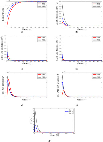Figure 1. The numerical solutions of system (1) for ${\eta }_1=2.5\times {10}^{-9}$, ${\eta }_2=1\times {10}^{-11}$, and $\omega =8\times {10}^{-3}$ with initials Sets I–III. The healthy equilibrium $E_0=\left(4\times {10}^5,0,0,0,0,0,0\right)$ is GAS. The healthy epithelial cells stabilize at $4\times {10}^5$, while all other components tend to 0.

(2)

We choose ${\eta }_1=2.5\times {10}^{-7}$, ${\eta }_2=1\times {10}^{-11}$, and $\omega =8\times {10}^{-7}$ to obtain ${\mathcal{R}}_0=19.2308>1$, ${\displaystyle \frac{{\mathcal{R}}_1}{{\mathcal{R}}_0}}=0.0243<1$, and ${\mathcal{R}}_2=0.0638<1$. This is consistent with the result of Theorem 4 that the equilibrium $E_1=$ (20,800, 9480, 7584, 0, 729,231, 0, 0) is GAS (Figure 2). In this case, the patient suffers from TB mono-infection while the CTL immunity is not active.

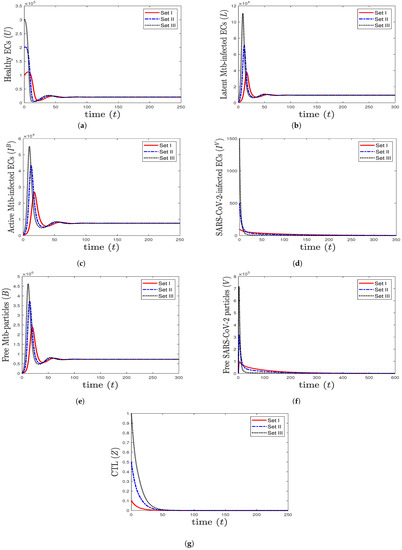Figure 2. The numerical solutions of system (1) for ${\eta }_1=2.5\times {10}^{-7}$, ${\eta }_2=1\times {10}^{-11}$, and $\omega =8\times {10}^{-7}$ with initials Sets I–III. The equilibrium $E_1=$ (20,800, 9480, 7584, 0, 729,231, 0, 0) is GAS. When TB mono-infection occurs, the components ($U,L,I^B,B$) stabilize at certain values, while all other components tend to 0.

(3)

We consider ${\eta }_1=2.5\times {10}^{-9}$, ${\eta }_2=1\times {10}^{-9}$, and $\omega =1\times {10}^{-8}$. This yields ${\mathcal{R}}_1=46.6667>1$, ${\displaystyle \frac{{\mathcal{R}}_0}{{\mathcal{R}}_1}}=0.0041<1$, and ${\mathcal{R}}_3=0.04<1$. These values lead to the global asymptotic stability of the equilibrium $E_2=$ (8571.43, 0, 0, 391,429, 0, $4.56667\times {10}^8$, 0), which agrees with the result of Theorem 5 (Figure 3). In this situation, the patient has SARS-CoV-2 mono-infection, where the CTL immunity is not present.

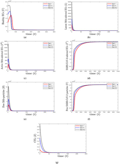Figure 3. The numerical solutions of system (1) for ${\eta }_1=2.5\times {10}^{-9}$, ${\eta }_2=1\times {10}^{-9}$, and $\omega =1\times {10}^{-8}$ with initials Sets I–III. The equilibrium $E_2=\left(8571.43,0,0,\mathrm{391,429},0,4.56667\times {10}^8,0\right)$ is GAS. When SARS-CoV-2 mono-infection occurs, the components ($U,I^V,V$) stabilize at certain values, while all other components tend to 0.

(4)

We select ${\eta }_1=2.5\times {10}^{-7}$, ${\eta }_2=1\times {10}^{-11}$, and $\omega =1\times {10}^{-}4$. This gives ${\mathcal{R}}_2=5.6497>1$ and ${\displaystyle \frac{(1-\xi )\lambda \omega {\eta }_2{\mu }_2{ϵ}_4}{{ϵ}_2{ϵ}_5\left[(1-\xi )\omega {ϵ}_1{ϵ}_4+{\eta }_1{\mu }_1{ϵ}_2{ϵ}_6\right]}}+1=1.0027<5.6697={\displaystyle \frac{{ϵ}_3}{{ϵ}_2}}+{\mathcal{R}}_2$. This implies that the equilibrium $E_3=$ ( 117,514, 7062.15, 1000, 0, 96,153.8, 0, 4.64972) is GAS (Figure 4), which is in complete agreement with Theorem 6. At this point, the CTL immune response is activated to eliminate TB disease from the body. As a result, the concentrations of Mtb-infected cells and Mtb particles are decreased, while the concentration of healthy cells is increased.

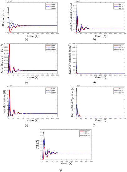Figure 4. The numerical solutions of system (1) for ${\eta }_1=2.5\times {10}^{-7}$, ${\eta }_2=1\times {10}^{-11}$, and $\omega =1\times {10}^{-4}$ with initials Sets I–III. The equilibrium $E_3=$ (117,514, 7062.15, 1000, 0, 96,153.8, 0, 4.64972) is GAS. The CTL immunity is activated to eliminate TB mono-infection, so the components ($U,L,I^B,B,Z$) stabilize at certain values, while all other components approach zero.

(5)

We choose ${\eta }_1=2.5\times {10}^{-9}$, ${\eta }_2=1\times {10}^{-9}$, and $\omega =1\times {10}^{-6}$. This generates the values ${\mathcal{R}}_3=3.6842>1$ and ${\displaystyle \frac{(1-\xi )\lambda \omega {\eta }_1{\mu }_1{ϵ}_2{ϵ}_5}{{ϵ}_3{ϵ}_4\left[(1-\xi )\omega {ϵ}_1{ϵ}_5+{\eta }_2{\mu }_2{ϵ}_6\right]}}+1=1.7591<53.6842={\displaystyle \frac{{ϵ}_2}{{ϵ}_3}}+{\mathcal{R}}_3$. In agreement with Theorem 7, the equilibrium $E_4=$ (31,578.9, 0, 0, $1\times {10}^5$, 0, $1.16667\times {10}^8$, 0.05368) is GAS (Figure 5). This point simulates the case of a COVID-19 patient with active CTL immunity that works to extract SARS-CoV-2 from the body.

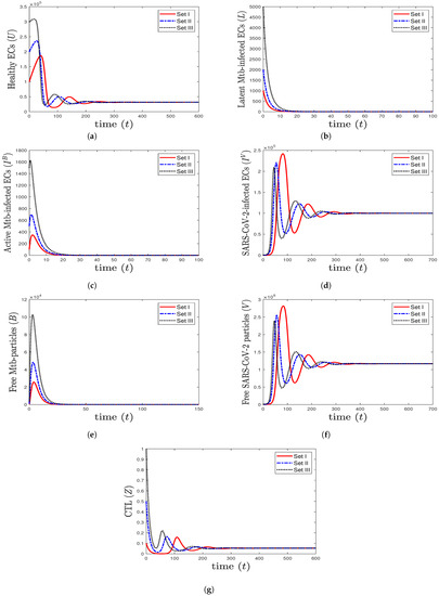Figure 5. The numerical solutions of system (1) for ${\eta }_1=2.5\times {10}^{-9}$, ${\eta }_2=1\times {10}^{-9}$, and $\omega =1\times {10}^{-6}$ with initials Sets I–III. The equilibrium $E_4=$ (31,578.9, 0, 0, $1\times {10}^5$, 0, $1.16667\times {10}^8$, 0.0536842) is GAS. The CTL immunity is activated to eliminate SARS-CoV-2 mono-infection, so the components ($U,I^V,V,Z$) stabilize at certain values, while all other components approach zero.

(6)

We take ${\eta }_1=2\times {10}^{-7}$, ${\eta }_2=1\times {10}^{-9}$, and $\omega =2\times {10}^{-6}$. These values give ${\displaystyle \frac{(1-\xi )\lambda \omega {\eta }_2{\mu }_2{ϵ}_4}{{ϵ}_2{ϵ}_5\left[(1-\xi )\omega {ϵ}_1{ϵ}_4+{\eta }_1{\mu }_1{ϵ}_2{ϵ}_6\right]}}+1=1.0096>0.1784={\displaystyle \frac{{ϵ}_3}{{ϵ}_2}}+{\mathcal{R}}_2$, ${\displaystyle \frac{(1-\xi )\lambda \omega {\eta }_1{\mu }_1{ϵ}_2{ϵ}_5}{{ϵ}_3{ϵ}_4\left[(1-\xi )\omega {ϵ}_1{ϵ}_5+{\eta }_2{\mu }_2{ϵ}_6\right]}}+1=113.5704>56.8293={\displaystyle \frac{{ϵ}_2}{{ϵ}_3}}+{\mathcal{R}}_3$, ${\displaystyle \frac{{\mathcal{R}}_1}{{\mathcal{R}}_0}}=3.0333>1$, and ${\displaystyle \frac{{\eta }_1{\mu }_1{ϵ}_2{ϵ}_5}{{\eta }_2{\mu }_2{ϵ}_4}}=16.4835>1$. This leads to the global asymptotic stability of the equilibrium $E_5=$ ( 27,125.6, 5712.6, 4380.44, 45,619.6, 421,196, $5.322\times {10}^7$, 0.043), which is compatible with the result of Theorem 8 (Figure 6). In this case, the patient suffers from TB and SARS-CoV-2 coinfection in the presence of CTL immunity.

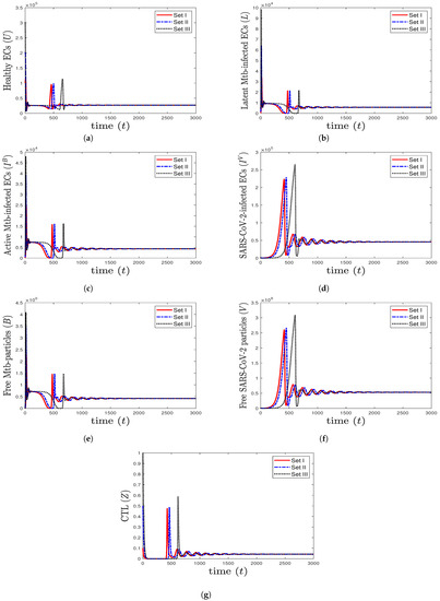Figure 6. The numerical solutions of system (1) for ${\eta }_1=2\times {10}^{-7}$, ${\eta }_2=1\times {10}^{-9}$, and $\omega =2\times {10}^{-6}$ with initials Sets I–III. The equilibrium $E_5=$ (27,125.6, 5712.6, 4380.44, 45,619.6, 421,196, $5.322\times {10}^7$, 0.043) is GAS. The TB and SARS-CoV-2 coinfection occurs with active immune response, so all components stabilize at certain values.

Table 1. Model parameters.

Parameter	Description	Value	Reference
$\lambda$	Recruitment rate of healthy ECs	$4\times {10}^3$	[39]
${\eta }_1$	Infection rate constant of ECs by Mtb	Varied	–
${\eta }_2$	Infection rate constant of ECs by SARS-CoV-2	Varied	–
a	Activation rate constant of latent Mtb-infected ECs	0.4	[15]
$\gamma$	Killing rate constant of infected ECs by CTLs	0.5	[14]
${\mu }_1$	Number of Mtb particles released per Mtb-infected cell	100	[16]
${\mu }_2$	Production rate constant of SARS-CoV-2 by SARS-CoV-2 infected ECss	700	[39]
$\xi$	Impact of lymphopenia on CTL immunity	$0\le \xi <1$	–
$\omega$	Stimulation rate constant of CTLs	Varied	–
${ϵ}_1$	Death rate constant of ECs	0.01	[39]
${ϵ}_2$	Death rate constant of Mtb-infected ECs	0.5	[16]
${ϵ}_3$	Death rate constant of SARS-CoV-2-infected ECs	0.01	[39]
${ϵ}_4$	Death rate constant of Mtb	0.52	[18]
${ϵ}_5$	Death rate constant of SARS-CoV-2	0.6	[26]
${ϵ}_6$	Death rate constant of CTLs	0.1	[39]

Table 1. Model parameters.

Parameter	Description	Value	Reference
$\lambda$	Recruitment rate of healthy ECs	$4\times {10}^3$	[39]
${\eta }_1$	Infection rate constant of ECs by Mtb	Varied	–
${\eta }_2$	Infection rate constant of ECs by SARS-CoV-2	Varied	–
a	Activation rate constant of latent Mtb-infected ECs	0.4	[15]
$\gamma$	Killing rate constant of infected ECs by CTLs	0.5	[14]
${\mu }_1$	Number of Mtb particles released per Mtb-infected cell	100	[16]
${\mu }_2$	Production rate constant of SARS-CoV-2 by SARS-CoV-2 infected ECss	700	[39]
$\xi$	Impact of lymphopenia on CTL immunity	$0\le \xi <1$	–
$\omega$	Stimulation rate constant of CTLs	Varied	–
${ϵ}_1$	Death rate constant of ECs	0.01	[39]
${ϵ}_2$	Death rate constant of Mtb-infected ECs	0.5	[16]
${ϵ}_3$	Death rate constant of SARS-CoV-2-infected ECs	0.01	[39]
${ϵ}_4$	Death rate constant of Mtb	0.52	[18]
${ϵ}_5$	Death rate constant of SARS-CoV-2	0.6	[26]
${ϵ}_6$	Death rate constant of CTLs	0.1	[39]

The Effect of Lymphopenia on SARS-CoV-2

To see the impact of lymphopenia that occurs during coinfection on SARS-CoV-2, we take the same values considered in case (6) and increase the value of $\xi$ to 0.5. We observe from Figure 7 that increasing the value of $\xi$ increases the concentration of SARS-CoV-2 particles. This means that lymphopenia, which decreases the efficacy of CTL immune response, enhances the production of SARS-CoV-2. Consequently, the health status of the coinfected patient can get worse.

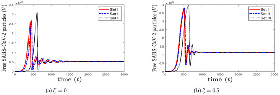
Figure 7. The impact of increasing $\xi$ (lymphopenia) on the concentration of SARS-CoV-2 particles.

6. Discussion and Future Works

In this work, we introduced an in-host TB and SARS-CoV-2 coinfection model. The model consists of seven ODEs that emulate the in-host interactions between healthy ECs, latent Mtb-infected ECs, active Mtb-infected ECs, SARS-CoV-2-infected ECs, free Mtb particles, free SARS-CoV-2 particles, and CTLs. It admits six equilibria as follows:

(1)

The healthy equilibrium $E_0$ always exists. It is GAS if ${\mathcal{R}}_0\le 1$ and ${\mathcal{R}}_1\le 1$. This state simulates the situation of a healthy person who does not suffer from TB and SARS-CoV-2 infections.

(2)

The Mtb mono-infection equilibrium with inactive CTLs $E_1$ exists if ${\mathcal{R}}_0>1$, while it is GAS if ${\displaystyle \frac{{\mathcal{R}}_1}{{\mathcal{R}}_0}}\le 1$ and ${\mathcal{R}}_2\le 1$. The patient here has Mtb mono-infection with inactive CTL immunity.

(3)

The SARS-CoV-2 mono-infection equilibrium with inactive CTLs $E_2$ exists if ${\mathcal{R}}_1>1$. It is GAS if ${\displaystyle \frac{{\mathcal{R}}_0}{{\mathcal{R}}_1}}\le 1$ and ${\mathcal{R}}_3\le 1$. In this state, the patient has SARS-CoV-2 mono-infection with inactive CTL immunity.

(4)

The Mtb mono-infection equilibrium with active CTLs $E_3$ exists if ${\mathcal{R}}_2>1$, while it is GAS if ${\displaystyle \frac{(1-\xi )\lambda \omega {\eta }_2{\mu }_2{ϵ}_4}{{ϵ}_2{ϵ}_5\left[(1-\xi )\omega {ϵ}_1{ϵ}_4+{\eta }_1{\mu }_1{ϵ}_2{ϵ}_6\right]}}+1\le {\displaystyle \frac{{ϵ}_3}{{ϵ}_2}}+{\mathcal{R}}_2$. In this situation, the CTL immune response is activated to extract Mtb infection from the body.

(5)

The SARS-CoV-2 mono-infection equilibrium with active CTLs $E_4$ exists if ${\mathcal{R}}_3>1$, and it is GAS if ${\displaystyle \frac{(1-\xi )\lambda \omega {\eta }_1{\mu }_1{ϵ}_2{ϵ}_5}{{ϵ}_3{ϵ}_4\left[(1-\xi )\omega {ϵ}_1{ϵ}_5+{\eta }_2{\mu }_2{ϵ}_6\right]}}+1\le {\displaystyle \frac{{ϵ}_2}{{ϵ}_3}}+{\mathcal{R}}_3$. This imitates the situation of a patient with SARS-CoV-2 mono-infection and active CTL immunity.

(6)

The Mtb and SARS-CoV-2 coinfection equilibrium with active CTLs $E_5$ exists, and it is GAS if ${\displaystyle \frac{(1-\xi )\lambda \omega {\eta }_2{\mu }_2{ϵ}_4}{{ϵ}_2{ϵ}_5\left[(1-\xi )\omega {ϵ}_1{ϵ}_4+{\eta }_1{\mu }_1{ϵ}_2{ϵ}_6\right]}}+1>{\displaystyle \frac{{ϵ}_3}{{ϵ}_2}}+{\mathcal{R}}_2$, ${\displaystyle \frac{(1-\xi )\lambda \omega {\eta }_1{\mu }_1{ϵ}_2{ϵ}_5}{{ϵ}_3{ϵ}_4\left[(1-\xi )\omega {ϵ}_1{ϵ}_5+{\eta }_2{\mu }_2{ϵ}_6\right]}}+1>{\displaystyle \frac{{ϵ}_2}{{ϵ}_3}}+{\mathcal{R}}_3$, ${\displaystyle \frac{{\mathcal{R}}_1}{{\mathcal{R}}_0}}>1$, ${ϵ}_2>{ϵ}_3$, and ${\displaystyle \frac{{\eta }_1{\mu }_1{ϵ}_2{ϵ}_5}{{\eta }_2{\mu }_2{ϵ}_4}}>1$. The patient here suffers from TB and SARS-CoV-2 coinfection and its consequences.

We found that the numerical results are fully compatible with the theoretical contributions. Model (1) can reflect three different states: (1) the healthy state where the person does not suffer from any infections, (2) the mono-infection state where the person has either TB infection or SARS-CoV-2 infection, and (3) the coinfection state where the person has TB and SARS-CoV-2 infections. These cases are reflected by the equilibria computed in Theorem 2. The movement between these states is determined by the threshold conditions. As these conditions depend on the parameters of model (1), their values should be carefully chosen. In addition, lymphopenia can worsen the health status of the coinfected patients because it causes a rise in the concentration of SARS-CoV-2 particles. In fact, lymphopenia has been observed in TB and SARS-CoV-2 coinfected patients [2,9]. Thus, it is a significant factor that needs to be determined and controlled. The model developed in this work can be used to understand the dynamics of coinfection and the role of immunity in increasing or decreasing the severity of the disease. This can support medical and experimental studies in promoting effective treatments for this class of patients. Indeed, the data on TB and SARS-CoV-2 is still very limited, and the effect of coinfection requires further study. The main limitation of this work is that we did not fit the model with real data to estimate the values of the parameters due to the scarcity of coinfection real data. We took the values from previous works that study SARS-CoV-2 or Mtb as single infections. Thus, this work can be developed by

(i)

Estimating the parameters’ values of model (1) by fitting with real data,

(ii)

Evaluating the proposed model with real data,

(iii)

Adding one compartment that shows the role of the antibody immune response in eliminating Mtb or SARS-CoV-2 particles,

(iv)

Inserting the effect of some treatments on coinfection, and

(v)

Considering the effect of CTL immunity with different killing and stimulation rates.

7. Conclusions

We found that the model investigated in this paper has two infection states:

(1)

The mono-infection state where the person has either TB or SARS-CoV-2 infection.

(2)

The coinfection state where the person has TB and SARS-CoV-2 infections.

The movement between these states depends on the fulfillment of threshold conditions and the values of the parameters. We also found that lymphopenia can cause a rise in the number of SARS-CoV-2 particles and may worsen the health status of the coinfected patient. Our model can be improved, and the results need to be tested when real data become obtainable.

References

- Coronavirus Disease (COVID-19), Weekly Epidemiological Update (8 January 2023). World Health Organization (WHO). 2023. Available online: https://www.who.int/publications/m/item/weekly-epidemiological-update-on-covid-19—11-january-2023 (accessed on 12 January 2023).
- Song, W.M.; Zhao, J.Y.; Zhang, Q.Y.; Liu, S.Q.; Zhu, X.H.; An, Q.Q.; Xu, T.T.; Li, S.J.; Liu, J.Y.; Tao, N.N.; et al. COVID-19 and Tuberculosis coinfection: An overview of case reports/case series and meta-analysis. Front. Med. 2021, 8, 1–13. [Google Scholar] [CrossRef]
- Tuberculosis, Fact Sheets. World Health Organization (WHO). 2022. Available online: https://www.who.int/news-room/fact-sheets/detail/tuberculosis (accessed on 12 January 2023).
- Shah, T.; Shah, Z.; Yasmeen, N.; Baloch, Z.; Xia, X. Pathogenesis of SARS-CoV-2 and Mycobacterium tuberculosis coinfection. Front. Immunol. 2022, 13, 1–17. [Google Scholar] [CrossRef]
- Luke, E.; Swafford, K.; Shirazi, G.; Venketaraman, V. TB and COVID-19: An exploration of the characteristics and resulting complications of co-infection. Front. Biosci. Sch. 2022, 14, 1–11. [Google Scholar] [CrossRef]
- Gatechompol, S.; Avihingsanon, A.; Putcharoen, O.; Ruxrungtham, K.; Kuritzkes, D.R. COVID-19 and HIV infection co-pandemics and their impact: A review of the literature. AIDS Res. Ther. 2021, 18, 28. [Google Scholar] [CrossRef]
- Shariq, M.; Sheikh, J.; Quadir, N.; Sharma, N.; Hasnain, S.; Ehtesham, N. COVID-19 and tuberculosis: The double whammy of respiratory pathogens. Eur. Respir. Rev. 2022, 31, 1–8. [Google Scholar] [CrossRef]
- Tapela, K.; Olwal, C.O.; Quaye, O. Parallels in the pathogenesis of SARS-CoV-2 and M. tuberculosis: A synergistic or antagonistic alliance? Future Microbiol. 2020, 15, 1691–1695. [Google Scholar] [CrossRef]
- Petrone, L.; Petruccioli, E.; Vanini, V.; Cuzzi, G.; Gualano, G.; Vittozzi, P.; Nicastri, E.; Maffongelli, G.; Grifoni, A.; Sette, A.; et al. Coinfection of tuberculosis and COVID-19 limits the ability to in vitro respond to SARS-CoV-2. Int. J. Infect. Dis. 2021, 113, S82–S87. [Google Scholar] [CrossRef]
- Blower, S.M.; Mclean, A.R.; Porco, T.C.; Small, P.M.; Hopewell, P.C.; Sanchez, M.A.; Moss, A.R. The intrinsic transmission dynamics of tuberculosis epidemics. Nat. Med. 1995, 1, 815–821. [Google Scholar] [CrossRef]
- Castillo-Chavez, C.; Feng, Z. To treat or not to treat: The case of tuberculosis. J. Math. Biol. 1997, 35, 629–656. [Google Scholar] [CrossRef]
- Feng, Z.; Castillo-Chavez, C.; Capurro, A. A model for tuberculosis with exogenous reinfection. Theor. Popul. Biol. 2000, 57, 235–247. [Google Scholar] [CrossRef]
- Castillo-Chavez, C.; Song, B. Dynamical models of tuberculosis and their applications. Math. Biosci. Eng. 2004, 1, 361–404. [Google Scholar] [CrossRef]
- Du, Y.; Wu, J.; Heffernan, J. A simple in-host model for Mycobacterium tuberculosis that captures all infection outcomes. Math. Popul. Stud. 2017, 24, 37–63. [Google Scholar] [CrossRef]
- He, D.; Wang, Q.; Lo, W. Mathematical analysis of macrophage-bacteria interaction in tuberculosis infection. Discret. Contin. Dyn. Syst. Ser. B 2018, 23, 3387–3413. [Google Scholar] [CrossRef]
- Yao, M.; Zhang, Y.; Wang, W. Bifurcation analysis for an in-host Mycobacterium tuberculosis model. Discret. Contin. Dyn. Syst. Ser. B 2021, 26, 2299–2322. [Google Scholar] [CrossRef]
- Zhang, W. Analysis of an in-host tuberculosis model for disease control. Appl. Math. Lett. 2020, 99, 1–7. [Google Scholar] [CrossRef]
- Ibarguen-Mondragon, E.; Esteva, L.; Burbano-Rosero, E. Mathematical model for the growth of Mycobacterium tuberculosis in the granuloma. Math. Biosci. Eng. 2018, 15, 407–428. [Google Scholar]
- Liang, K. Mathematical model of infection kinetics and its analysis for COVID-19, SARS and MERS. Infect. Genet. Evol. 2020, 82, 104306. [Google Scholar] [CrossRef]
- Krishna, M.V. Mathematical modelling on diffusion and control of COVID-19. Infect. Dis. Model. 2020, 5, 588–597. [Google Scholar] [CrossRef]
- Ivorra, B.; Ferrandez, M.R.; Vela-Perez, M.; Ramos, A.M. Mathematical modeling of the spread of the coronavirus disease 2019 (COVID-19) taking into account the undetected infections. The case of China. Commun. Nonlinear Sci. Numer. Simul. 2020, 88, 105303. [Google Scholar] [CrossRef]
- Yang, C.; Wang, J. A mathematical model for the novel coronavirus epidemic in Wuhan, China. Math. Biosci. Eng. 2020, 17, 2708–2724. [Google Scholar] [CrossRef]
- Krishna, M.V.; Prakash, J. Mathematical modelling on phase based transmissibility of Coronavirus. Infect. Dis. Model. 2020, 5, 375–385. [Google Scholar] [CrossRef]
- Rajagopal, K.; Hasanzadeh, N.; Parastesh, F.; Hamarash, I.I.; Jafari, S.; Hussain, I. A fractional-order model for the novel coronavirus (COVID-19) outbreak. Nonlinear Dyn. 2020, 101, 711–718. [Google Scholar] [CrossRef]
- Chen, T.M.; Rui, J.; Wang, Q.P.; Zhao, Z.Y.; Cui, J.A.; Yin, L. A mathematical model for simulating the phase-based transmissibility of a novel coronavirus. Infect. Dis. Poverty 2020, 9, 1–8. [Google Scholar] [CrossRef]
- Almocera, A.S.; Quiroz, G.; Hernandez-Vargas, E.A. Stability analysis in COVID-19 within-host model with immune response. Commun. Nonlinear Sci. Numer. Simul. 2020, 95, 105584. [Google Scholar] [CrossRef]
- Hernandez-Vargas, E.A.; Velasco-Hernandez, J.X. In-host mathematical modeling of COVID-19 in humans. Annu. Rev. Control 2020, 50, 448–456. [Google Scholar] [CrossRef]
- Li, C.; Xu, J.; Liu, J.; Zhou, Y. The within-host viral kinetics of SARS-CoV-2. Math. Biosci. Eng. 2020, 17, 2853–2861. [Google Scholar] [CrossRef]
- Agha, A.D.A.; Elaiw, A.M. Global dynamics of SARS-CoV-2/malaria model with antibody immune response. Math. Biosci. Eng. 2022, 19, 8380–8410. [Google Scholar] [CrossRef]
- Pinky, L.; Dobrovolny, H.M. SARS-CoV-2 coinfections: Could influenza and the common cold be beneficial? J. Med. Virol. 2020, 92, 2623–2630. [Google Scholar] [CrossRef]
- Elaiw, A.M.; Agha, A.D.A.; Azoz, S.A.; Ramadan, E. Global analysis of within-host SARS-CoV-2/HIV coinfection model with latency. Eur. Phys. J. Plus 2022, 137, 1–22. [Google Scholar] [CrossRef]
- Ahmed, I.; Goufo, E.F.D.; Yusuf, A.; Kumam, P.; Chaipanya, P.; Nonlaopon, K. An epidemic prediction from analysis of a combined HIV-COVID-19 co-infection model via ABC-fractional operator. Alex. Eng. J. 2021, 60, 2979–2995. [Google Scholar] [CrossRef]
- Omame, A.; Abbas, M.; Abdel-Aty, A. Assessing the impact of SARS-CoV-2 infection on the dynamics of dengue and HIV via fractional derivative. Chaos Solitons Fractals 2022, 162, 1–22. [Google Scholar] [CrossRef]
- Mekonen, K.; Balcha, S.; Obsu, L.; Hassen, A. Mathematical modeling and analysis of TB and COVID-19 coinfection. J. Appl. Math. 2022, 2022, 1–20. [Google Scholar] [CrossRef]
- Bandekar, S.; Ghosh, M. A co-infection model on TB—COVID-19 with optimal control and sensitivity analysis. Math. Comput. Simul. 2022, 200, 1–31. [Google Scholar] [CrossRef]
- Marimuthu, Y.; Nagappa, B.; Sharma, N.; Basu, S.; Chopra, K. COVID-19 and tuberculosis: A mathematical model based forecasting in Delhi, India. Indian J. Tuberc. 2020, 67, 177–181. [Google Scholar] [CrossRef]
- Rwezaura, H.; Diagne, M.L.; Omame, A.; de Espindola, A.L.; Tchuenche, J.M. Mathematical modeling and optimal control of SARS-CoV-2 and tuberculosis co-infection: A case study of Indonesia. Model. Earth Syst. Environ. 2022, 8, 5493–5520. [Google Scholar] [CrossRef]
- Khalil, H.K. Nonlinear Systems; Prentice-Hall: Hoboken, NJ, USA, 1996. [Google Scholar]
- Sumi, T.; Harada, K. Immune response to SARS-CoV-2 in severe disease and long COVID-19. iScience 2022, 25, 1–18. [Google Scholar] [CrossRef]
Disclaimer/Publisher’s Note: The statements, opinions and data contained in all publications are solely those of the individual author(s) and contributor(s) and not of MDPI and/or the editor(s). MDPI and/or the editor(s) disclaim responsibility for any injury to people or property resulting from any ideas, methods, instructions or products referred to in the content. |
© 2023 by the authors. Licensee MDPI, Basel, Switzerland. This article is an open access article distributed under the terms and conditions of the Creative Commons Attribution (CC BY) license (https://creativecommons.org/licenses/by/4.0/).