Derivation of the Fractional Fokker–Planck Equation for Stable Lévy with Financial Applications

Abstract

This paper aims to propose a generalized fractional Fokker–Planck equation based on a stable Lévy stochastic process. To develop the general fractional equation, we will use the Lévy process rather than the Brownian motion. Due to the Lévy process, this fractional equation can provide a better description of heavy tails and skewness. The analytical solution is chosen to solve the fractional equation and is expressed using the H-function to demonstrate the indicator entropy production rate. We model market data using a stable distribution to demonstrate the relationships between the tails and the new fractional Fokker–Planck model, as well as develop an R code that can be used to draw figures from real data.

1. Introduction

Recently, there has been a development of fractional calculus theory and applications. There are many researchers in various areas concerning fractional calculus, and their studies have gained importance in different areas. For instance, in 1993 [1] and in 1998 [2], researchers studied the historical development of fractional calculus theory, and presented examples and theoretical applications. The paper [3] in 1998 studied the entropy production rate for fractional diffusion processes, which was obtained by applying the group method to the fractional differential equation and directly derived from invariant and non-invariant factors of the probability density function. The fundamental solutions of the fractional diffusion equation were studied and expressed in terms of proper Fox H functions [4]. In an earlier work, Aljedhi and Kılıçman [5] derived the corresponding general fractional partial differential equation using a specific Lévy anomalous diffusion equation as a model of asset values. The study [6] examined the sensitivity of the option price in relation to specific model parameters established in [5] and also looked at a numerical study of the value of European-style options of the specific model.

When the Gaussian Brownian algorithm is used in classic statistical description, for instance, the Fokker–Planck equation, which describes the time development of the probability density function, fails for many realistic issues. Furthermore, it is not always suitable to use the Gaussian distribution on the heavy tail of the stock market in systems with long time limits. For this case, the general fractional Lévy distributions Equation (1), which describe actual market data with a long-term limit and whose corresponding probability distribution function is defined by the fractional Fokker–Planck equation, ought to be taken into consideration.

The aim of this work is to derive a fractional time–space Fokker-Planck model from the specific general Lévy anomalous diffusion equation mentioned in [5]. We will establish a general model of the Fokker-Planck equation from the specific Lévy anomalous diffusion equation, where the Fokker–Planck equation is one of the most well-known equations in statistical physics. The Fokker–Planck equation was beneficial for concentrating on the stochastic differential equations’ dynamic behavior under the influence of Gaussian noise. The Fokker–Planck equation explains how the probability density function changes over time as a particle’s speed is influenced by irregular and drag forces, as in Brownian motion.

In the literature, Duan, et al. (2000) [7], because of the properties of the heavy tail and the central limit theorem, derived the fractional space Fokker–Planck equation of the probability distribution by a Levy-stable noise rather than a Gaussian with the aid of the Laplacian derivative’s fractional powers. (Yanovsky, et al. (2000) [8]) derived fractional Fokker–Planck equation by Lévy anomalous diffusion. They derived the fractional Fokker–Planck equation, which has a fractional space derivative instead of the standard Laplacian derivative using the distribution function of the generalized Langevin equation. In this paper, we established the general fractional time–space Fokker–Planck equation from the non-Gaussian equation, which includes anomalous diffusion because of a Lévy $\alpha$-stable process. Consequently, we will demonstrate that the fundamental solution to the (FFPE) has a different entropy production rate when compared to the conventional diffusion equation. The entropy of the diffusion processes and the rate at which it is produced are two other crucial characteristics. Macroscopic thermodynamics presented the idea of entropy first, and later Information theory, ergodic theory of dynamical systems, mechanical statistics, and other fields expanded it to describe specific occurrences. Entropy has been defined in a variety of ways throughout history and used in a variety of fields of knowledge. Shannon created the statistical notion of entropy, which is used in this study. The study [3,9,10] discussed the entropy of the diffusion equations governed by the space-fractional diffusion equations.

Consider $L_t^{\alpha ,\eta }$ to be a Lévy process with asset price’s $S_t$ as a risk-neutral probability measure, as described in Aljedhi and Kılıçman [5] and Lewis [11] is the following time-fractional stochastic differential equation with boundary condition of the Lévy process,

$$d^{\gamma }{S}_t=\left(md{t}^{\gamma }+\sigma d{L}_t^{\alpha ,\eta }\right)S_t,S(0)=S_0$$

(1)

where $m\in R,\sigma >0$, $\gamma \in (0,1]$, $t\in (0,T]$, $\eta \in [-1,1]$ and $\alpha \in (1,2)$.

The Lévy process $L_t^{\alpha ,\eta }$ has a characteristic function represented as:

$$E\left[e^{ik{X}_t}\right]=e^{t\psi (k)}$$

(2)

with

$$\psi (k)=mik-\frac{1}{2}{\sigma }^2{k}^2+{\int }_{R\setminus 0}(e^{ikx}-1-ik{I}_{|x|<1})\nu (dx)$$

(3)

m is a real number, $\sigma \ge 0$, and the indicator function I, ${\int }_R{[1,x^2]}^{+}\nu (dx)<\infty$ and $\nu =w(x)$ is Lévy density. Consider $w(x)=w_{LS}(x)$ Lévy density function given by

$$w_{LS}=\left\{\begin{array}{cc}\frac{b}{{\left|x\right|}^{1+\alpha }}& \mathrm{for}x<0\\ \frac{c}{x^{1+\alpha }}& \mathrm{for}x>0\end{array}\right.$$

where $b+c=1$ and $\alpha \in (0,2)$. Using $w_{LS}(x)$ to obtain the characteristic Lévy stable formula

$${\Psi }_{LS}(k)=ikm-\frac{{\sigma }^{\alpha }}{2}{\left|k\right|}^{\alpha }\left[1-i\eta {\phi }_{(\alpha ,k)}sign(k)\right].$$

The function $\phi (k,\alpha )$ can be defined as

$${\phi }_{(\alpha ,k)}=\left\{\begin{array}{cc}tan(\frac{\pi \alpha }{2})\hfill & ,\alpha \ne 1\hfill \\ \frac{\pi log|k|}{2}\hfill & ,\alpha =1\hfill \end{array}\right.$$

for $\alpha \ne 1$, we have

$${\Psi }_{LS}(k)=ikm-\frac{{\sigma }^{\alpha }}{2}{\left|k\right|}^{\alpha }\left[1-i\eta sign(k)tan\left(\frac{\alpha \pi }{2}\right)\right]$$

or equivalent [11,12]

$$\Psi (k)=ikm-\frac{{\sigma }^{\alpha }}{4cos(\frac{\alpha \pi }{2})}\left[\left(1-\eta \right){(ik)}^{\alpha }+\left(1+\eta )\right){(-ik)}^{\alpha }\right]$$

(4)

where $\eta =c-b$. The parameter $\eta$ characterizes the degree of a symmetry. Indeed, if $\eta =0$, there is an occurrence of equal probabilities of $\eta (t)$ with positive and negative values of $\eta (t)$. While $\eta =-1$ left maximal symmetric distribution, if $\eta =1$ right maximal symmetric distribution. In the symmetric case when $\eta =0$, Figure 1 compares the tail behavior of Geometric Brownian motion and Lévy stable distributions, with select ($m=0$ and $\sigma =1$). When $\alpha =2$, the Lévy stable is a normal distribution with mean m and standard deviation $\frac{\sigma }{\sqrt{2}}$. It is observed that the tails get heavier when $\alpha$ decreases. The shape of the tails for the real data ($S\&P500$) at various values of $\alpha$ is depicted in Figure 3 in Section 5.

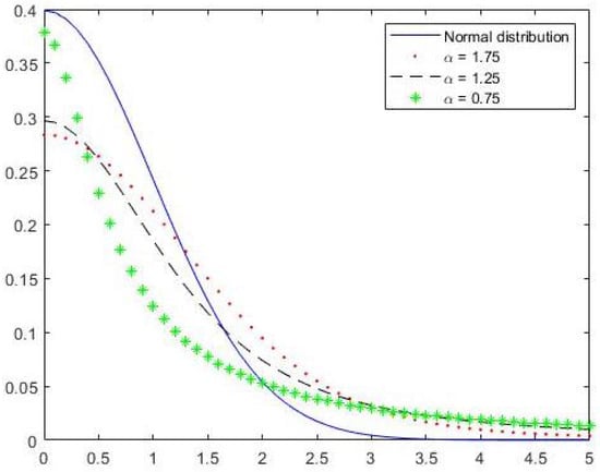
Figure 1. Comparing the tail behavior of Brownian motion of ($\alpha =2$) and Lévy stable of Equation (4) at varying value of $\alpha$, with $m=0$ and $\sigma =1$. It can be observed that the tails get heavier when $\alpha$ decreases.

The primary goal is to use Lévy motions to extend the Fokker–Planck equation to the generalized fractional Fokker–Planck equation. This will be achieved by expanding on previous works [7,13,14,15], thereby demonstrating that a generalized FFPE, including fractional derivatives, is satisfied by the probability density of particles traveling with a Lévy process. See some early related studies in [16,17,18,19,20,21].

The paper is based on the following: Section 2 derives the fractional Fokker–Planck equation with alpha stable process. Section 3 finds the analytical solution and Mellin integral representation of the equation derived in the previous section. Section 4 estimates the entropy production rate while adopting the Shannon definition of the entropy. Section 5 focuses on the financial applications and estimates $\alpha$ stable in Section 1. Finally, Section 6 concludes the article.

2. Fractional Fokker–Planck Equation

In the literature [8] derived the fractional Fokker–Planck equation (FFPE) by substituting a Lévy-stable process to the classical Gaussian one in the Langevin-like equation.

In this paper, the derivation of (FFPE) is based on the Lévy-stable fractional stochastic Equation (1) and the characteristic Lévy stable formula (4). First, we need the transition probability density function, [7] denoted by $\mathcal{P}(y,t;\acute{y},\acute{t})$, of the Lévy process,

$$\mathcal{P}(c<\acute{y}<d\mathrm{at}\acute{t}|y\mathrm{at}t)={\int }_c^d\mathcal{P}(\acute{y}|\acute{t})\mathcal{P}(y,t;\acute{y},\acute{t})d\acute{y}$$

The density of particles diffuse from $(y,t)$ to $(\acute{y},\acute{t})$ [22]. That means the probability that the random variable $\acute{y}$ lies in the interval $(a,b)$, at a future time $\acute{t}$, given that it started at time t with value x.

Taking the special transition density $\mathcal{P}(y-y_1,\tau )$ with positive integer $n_T$ where $\tau =\frac{T-t}{n_T}$ and temporal grid points $t_k$ with uniform time step $t_k=t+k\tau$, $k=0,\dots ,n_T$.

Set shorter $\mathcal{P}(y,t)=\mathcal{P}(y-\acute{y}|t-\acute{t})$.

The particle density with the present position y at any time t can be formulated as

$$\mathcal{P}(y,t+\tau )=\int dz\mathcal{P}(z,t)\mathcal{P}(y-z|\tau )$$

(5)

The density of particles diffusing from $(y,t)$ to $(\acute{y},\acute{t})$ denotes the probability that the random variable $\acute{y}$ lies in the interval $(a,b)$, at a future time $\acute{t}$ given that it started out at time t with value y [22].

According to [22], an equation for the distribution function of transition probability density can be represented by the inverse Fourier transform of the characteristic function (2)

$$\mathcal{P}(y,t)={\int }_{-\infty }^{\infty }{e}^{-iky}{e}^{t\psi (k)}dk.$$

Thus

$$\mathcal{P}(y,t)={\mathcal{F}}^{-1}\left[e^{t\psi (k)}\right],$$

(6)

inverse Fourier transform ${\mathcal{F}}^{-1}$ defined as

$${\mathcal{F}}^{-1}\left[\mathcal{F}(k)\right]=f(x)=\frac{1}{2\pi }{\int }_{-\infty }^{\infty }{e}^{-ikx}\mathcal{F}(k)dk$$

where $\mathcal{F}$ is the Fourier transform and is defined as

$$\mathcal{F}[f(x);k]=\mathcal{F}(k)={\int }_{-\infty }^{\infty }{e}^{ikx}f(x)dx.$$

It is known that the definition of a first-order derivative of the function f is defined as

$$f^{\prime }(x)=\underset{h⟶0}{lim}\frac{1}{h}\left(f(x+h)-f(x)\right).$$

(7)

The Caputo derivative of order $0<\gamma \le 1$ is defined as

$$D_t^{\gamma }f(x)={\int }_0^t{f}^{(1)}(\xi ){(t-\xi )}^{-\gamma }\frac{d\xi }{\Gamma (1-\gamma )}$$

(8)

and the fractional integral has the expression

$$I^{\gamma }f(v)=\frac{1}{\Gamma \left(\gamma \right)}{\int }_{-\infty }^{v}f(\xi ){(v-\xi )}^{\gamma -1}d\xi .$$

where $\Gamma$ is the gamma function. Taking the fractional derivative of Equation (5), we obtain

$$D_t^{\gamma }p(y,t)={\int }_0^t{(t-\xi )}^{-\gamma }\underset{\tau ⟶0}{lim}\frac{\int p(y-x|\tau )p(x,\xi )dx-p(x,\xi )}{\tau }\frac{d\xi }{\Gamma (1-\gamma )}$$

(9)

where

$$p^{\prime }(y,t)=\underset{\tau ⟶0}{lim}\frac{\int p(y-x|\tau )p(y,\xi )dx-p(y,\xi )}{\tau }d\xi .$$

(10)

Taking Fourier transform and using convolution theorem with respect to x of Equation (9), obtaining

$$D_t^{\gamma }\tilde{p}(k,t)=\frac{1}{\Gamma (1-\gamma )}{\int }_0^t{(t-\xi )}^{-\gamma }\underset{\tau ⟶0}{lim}\frac{\int \tilde{p}(k,\xi )(\tilde{p}(k|\tau )-1)}{\tau }d\xi$$

(11)

where by the convolution Fourier Theorem,

$$\mathcal{F}\left[\int p(y-x|\tau )p(x,\xi )dx;k\right]=\tilde{p}(k,\xi )\tilde{p}(k|\tau ).$$

(12)

Equation (11) gives the relation between transition density and time, which is commonly assumed to be a linear relationship. For this linear scaling, select cumulant expansion of finite variance transition density [23].

$$\tilde{p}(k|\tau )=1+\sum _{k=1}^{\infty }{B}_k\frac{{(ik)}^k}{k}.$$

The stable transition density has the cumulant expansion

$$\tilde{p}(k|\tau )=1-m\tau (ik)+Ac\tau {(ik)}^{\alpha }+Ab\tau {(-ik)}^{\alpha }+o(\tau ).$$

(13)

The Fourier transform of the stable density

$$\tilde{p}(k|\tau )=exp(-m(ik)+Ac{(ik)}^{\alpha }+Ab{(-ik)}^{\alpha }),$$

(14)

substitute the expansion into Equation (9) and taking the limit

$$D_t^{\gamma }\tilde{p}(k,t)=\frac{1}{\Gamma (1-\gamma )}{\int }_0^t\frac{\tilde{p}(k,\xi )}{{(t-\xi )}^{\gamma }}(-m(ik)+Ac{(ik)}^{\alpha }+Ab{(-ik)}^{\alpha })d\xi .$$

(15)

The FFPE is derived from Equation (15) by inverting the Fourier transform. Inverse Fourier transform of fractional derivatives can be defined as [24],

$${\mathcal{F}}^{-1}\left[{(-ik)}^{\alpha }\widehat{G}(k)\right]{=}_{-\infty }{D}_x^{\alpha }g(y)$$

and

$${\mathcal{F}}^{-1}\left[{(ik)}^{\alpha }\widehat{G}(k)\right]{=}_x{D}_{\infty }^{\alpha }g(y)$$

where ${}_{-\infty }{D}_x^{\alpha }{,}_x{D}_{\infty }^{\alpha }$ are lift and right Riemann–Liouville fractional derivative of order $n-1\le \alpha \le n$ defined as

$${}_{-\infty }{D}_x^{\alpha }g(x)=\frac{{\partial }^n}{\partial x^n}{\int }_{-\infty }^x\frac{g(\xi )}{{(x-\xi )}^{\alpha -n+1}}\frac{d\xi }{\Gamma \left(n-\alpha \right)},$$

(16)

the right

$${}_x{D}_{\infty }^{\alpha }g(x)=\frac{{\partial }^n}{\partial x^n}{\int }_x^{\infty }{(\xi -x)}^{n-\alpha -1}g(\xi )\frac{d\xi {(-1)}^n}{\Gamma \left(n-\alpha \right)}$$

(17)

Thus, inverting the Fourier transform of Equation (15) and using staple density property in (4) will obtain the fractional Fokker–Planck equation,

$$D_t^{\gamma }\mathcal{P}(y,t)=-m\frac{\partial }{\partial x}\mathcal{P}(y,t)-\frac{{\sigma }^{\alpha }}{2cos(\frac{\alpha \pi }{2})}[{(1+\eta )}_{-\infty }{D}_y^{\alpha }+{(1-\eta )}_y{D}_{\infty }^{\alpha }]\mathcal{P}(y,t).$$

(18)

Refer to [25,26], the sum is given by the symmetry (in case $\eta =0)$

$$\frac{d^{\alpha }}{{d|y|}^{\alpha }}=-\frac{{\sigma }^{\alpha }}{2cos(\frac{\alpha \pi }{2})}[\frac{d^{\alpha }}{d{y}^{\alpha }}+\frac{d^{\alpha }}{d{(-y)}^{\alpha }}]$$

(19)

substituting Equation (19) into (18), we obtain

$$D_t^{\gamma }\mathcal{P}(y,t)=(-m\frac{\partial }{\partial y}+\frac{{\partial }^{\alpha }}{{\partial |y|}^{\alpha }})\mathcal{P}(y,t).$$

(20)

3. Fractional Fokker–Planck Analytical Solution

In this section, we present analytical solutions for Fokker–Planck fractions. The solution is expressed in terms of Fox H functions and Lévy stable distribution. The solution is obtained from the properties and asymptotic behavior of Fox H functions [27]. The FFPE (20) with initial condition

$$\mathcal{P}(y,0)=\delta (y)$$

(21)

where $\delta (y)$ is the dirac delta function. Regarding the Fourier transform

$$\mathcal{F}\left[P\right]=\tilde{P}={\int }_{-\infty }^{\infty }{e}^{iky}p(y)dy$$

this is easily the Fourier invert

$$\frac{{\partial }^{\alpha }p}{{\partial |y|}^{\alpha }}={\mathcal{F}}^{-1}{[-|k|}^{\alpha }\mathcal{F}\left[P\right]].$$

(22)

Explain the process by taking the Fourier transform with respect to y for the Equations (20) and (21).

$$D_t^{\gamma }\tilde{P}(k,t)=mik\tilde{P}(k,t)-{|k|}^{\alpha }\tilde{P}(k,t).$$

(23)

The exact solution of a particular fractional differential equation was obtained in [28] by transforming the analogous fractional Volterra integral equation of an integer order differential equation. By this method, the solution of Equation (23) is

$$\tilde{P}(k,t)={\tilde{P}}_1(k,\nu ),\nu =\frac{t^{\gamma }}{\Gamma (1+\gamma )}$$

(24)

where ${\tilde{P}}_1(k,\nu )$ is a solution of the ordinary differential equation

$$\frac{d{\tilde{P}}_1(k,\nu )}{d\nu }=g(\nu ,{\tilde{P}}_1(k,\nu ))=f(\tau ,{\tilde{P}}_1(k,\tau )),{\tilde{P}}_1(k,0)={\tilde{P}}_0$$

(25)

where

$$\frac{d^{\gamma }X(t)}{d{t}^{\gamma }}=f(x,X(t))$$

and

$$\tau =t-{(t^{\gamma }-\nu \Gamma (1+\gamma ))}^{\frac{1}{\gamma }}.$$

Thus (23) can be written using (24) and (25)

$$\frac{d{\tilde{P}}_1(k,\nu )}{d\nu }={[mik-|k|}^{\alpha }]{\tilde{P}}_1(k,\nu ).$$

(26)

The ordinary differential Equation (26) has the solution

$$\tilde{P}(k,t)={\tilde{P}}_1(k,\nu )={\tilde{P}}_0{exp(mik-|k|}^{\alpha }).$$

Invert Fourier transform and using Lévy stable distribution with parameter $1<\alpha <2$, we have

$$P_1(y,\nu )={\int }_{-\infty }^{\infty }{e}^{-iky}{e}^{ikm\nu }{exp(-|k|}^{\alpha }\nu )dk$$

(27)

then the solution $P_1(y,\nu )=\mathrm{u}(y-m,\nu )$ is defined by

$$\mathrm{u}(y-m,\nu )={\mathcal{F}}^{-1}\left[e^{-{|k|}^{\alpha }\nu }\right].$$

(28)

Rewrite (23) as Fourier cosine transform

$$\mathrm{u}(y,\nu )=\frac{1}{\pi }{\mathcal{F}}_c\left[e^{-{|k|}^{\alpha }\nu }\right].$$

(29)

Using representation of the Fox H function [4,29], and $\nu =\frac{t^{\gamma }}{\Gamma (1+\gamma )}$,

$$\begin{array}{cc}\hfill e^{-t^{\gamma }{|k|}^{\alpha }}=\frac{1}{\alpha }{H}_{0,1}^{1,0}& \left(\begin{array}{c}|y|t^{-\frac{\gamma }{\alpha }}\end{array}{\displaystyle |}\begin{array}{c}\\ (0,\frac{1}{\alpha })\end{array}\right).\hfill \end{array}$$

Fourier cosine transform of Fox H functions [30], when $1\le \alpha <2$

$$\begin{array}{cc}\hfill {\mathcal{F}}_c\left[H_{p,q}^{n,m}(z)\right](v)=\frac{\pi }{v}{H}_{p+2,q+1}^{m,n+1}& \left(\begin{array}{c}\frac{1}{v}\end{array}{\displaystyle |}\begin{array}{ccc}(1-b_j,{\beta }_j),& (1,\frac{1}{2})& \\ (1,1),& (a_j,{\vartheta }_j),& (1,\frac{1}{2})\end{array}\right).\hfill \end{array}$$

Therefore, (26) with (24) we have the solution of fractional Fokker–Planck

$$\begin{array}{cc}\hfill \mathrm{u}(y,t)=\frac{1}{\alpha |y|}{H}_{2,2}^{1,1}& \left(\begin{array}{c}{|y|(At)}^{-\frac{\gamma }{\alpha }}\end{array}{\displaystyle |}\begin{array}{cc}(1,\frac{1}{\alpha }),& (1,\frac{1}{2})\\ (1,1),& (1,\frac{1}{2})\end{array}\right)\hfill \end{array}$$

where we set $A^{\gamma }=\frac{1}{\Gamma (1+\gamma )}$. The Mellin–Barnes presentation [31].

$$\mathrm{u}(y,t)=\frac{1}{2\pi }\frac{1}{\alpha |y|}\int \frac{\Gamma (1-s)\Gamma (\frac{s}{\alpha })}{\Gamma (\frac{s}{2})\Gamma (1-\frac{s}{2})}{\left({|y|(At)}^{-\frac{\gamma }{\alpha }}\right)}^{s}ds.$$

(30)

Figure 2 shows the behavior of the analytical solution of the Fokker–Planck equation in the symmetric case for different values of $\alpha \in (1,2)$ and $\gamma =0.3$.

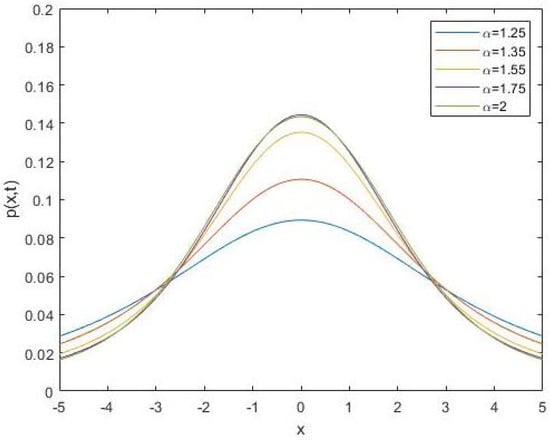
Figure 2. Analytical solution of (FFPE) of Equation (30) at different values of $\alpha =1.15,1.35,1.55,1.75$, and 2 around $x=0$, in the symmetric case with $\gamma =0.3$.

4. Entropy Production Rate

This section demonstrates how the Shannon entropy is a useful dynamical indicator that gives a clear indication of the diffusion rate and, consequently, a timescale for the instabilities that result from dealing with chaos. The Shannon entropy is defined with the probability density function $p(x,t)$

$$S(P,t)=-{\int }_{-\infty }^{\infty }p(x,t)ln(p(x,t)).$$

(31)

The entropy production rate defined by Shannon derivative

$$R(P,t)=\frac{dS(P,t)}{dt}.$$

(32)

In this paper we considered the FFPE with the Caputo time derivative with order $\gamma$.

To compute the entropy of the one-dimensional FFPE (20) from (28) is the characteristic function of stable distribution $C(x|\alpha ,\eta ,\delta ,m;n)$ with symmetric skewness and scaling property for $0<\alpha <2$, yield

$$u(y,t)=\mathcal{F}\left[e^{-{|k|}^{\alpha }{t}^{\frac{\gamma }{\alpha }}}\right]=C(y|\alpha ,0,t^{\frac{\gamma }{\alpha }},0;0)=t^{-\frac{\gamma }{\alpha }}C(y{t}^{-\frac{\gamma }{\alpha }}|\alpha ,0,1,0;0).$$

Thus, the above solution is written with the auxiliary function

$$G_{\alpha ,\gamma }(Z)=C(Z|\alpha ,0,1,0;0)$$

as

$$u(y,t)=t^{-\frac{\gamma }{\alpha }}{G}_{\alpha ,\gamma }(y{t}^{-\frac{\gamma }{\alpha }}).$$

(33)

Apply the Shannon entropy on Equation (33),

$$S(P,t)=-\int t^{-\frac{\gamma }{\alpha }}{G}_{\alpha ,\gamma }(y{t}^{-\frac{\gamma }{\alpha }})ln(t^{-\frac{\gamma }{\alpha }}{G}_{\alpha ,\gamma }(y{t}^{-\frac{\gamma }{\alpha }}))dy.$$

For the stability scaling behavior, we can set $z=y{t}^{-\frac{\gamma }{\alpha }}$ then $dz=dx{t}^{-\frac{\gamma }{\alpha }}$, and get

$$\begin{array}{cc}\hfill S(P,t)=& -{\int }_{-\infty }^{\infty }{G}_{\alpha ,\gamma }(z)ln(t^{-\frac{\gamma }{\alpha }}{G}_{\alpha ,\gamma }(z))dz\hfill \\ \hfill =& -{\int }_{-\infty }^{\infty }{G}_{\alpha ,\gamma }(z)[(-\frac{\gamma }{\alpha })ln(t)+ln(G_{\alpha ,\gamma }(z))]dz\hfill \\ \hfill =& (\frac{\gamma }{\alpha })ln(t){\int }_{-\infty }^{\infty }{G}_{\alpha ,\gamma }(z)dz-{\int }_{-\infty }^{\infty }{G}_{\alpha ,\gamma }(z)ln(G_{\alpha ,\gamma }(z))dz\hfill \end{array}$$

Which is ${\int }_{-\infty }^{\infty }{G}_{\alpha ,\gamma }(z)=1$ get

$$S(P,t)=(\frac{\gamma }{\alpha })ln(t)-A_{\alpha ,\gamma }$$

(34)

where

$$A_{\alpha ,\gamma }={\int }_{-\infty }^{\infty }{G}_{\alpha ,\gamma }(z)ln(G_{\alpha ,\gamma }(z))dz.$$

(35)

The entropy production rate is

$$R(t)=\frac{dS(P,t)}{dt}=(\frac{\gamma }{\alpha })\frac{1}{t}.$$

(36)

The calculation above demonstrates how $R(t)$ depends on the fractional order of the space-time. The Fokker–Planck equation differs from the entropy production rate of the traditional one-dimensional diffusion equation and the fractional one-dimensional diffusion equation [32] in that it is not reliant on the order.

5. Data and Results

Equation (30) defines the solution $\mathrm{u}(y,t)$ as an inverse transform of the Mellin integral form, which has the series expansion [4,31,33].

$$\begin{array}{cc}\hfill \mathrm{u}(y,t)=& \frac{1}{2i\pi }\frac{1}{\alpha |y|}\int \frac{\Gamma (1-s)\Gamma (\frac{s}{\alpha })}{\Gamma (\frac{s}{2})\Gamma (1-\frac{s}{2})}{\left({|y|(At)}^{-\frac{\gamma }{\alpha }}\right)}^{s}ds\hfill \\ \hfill =& \frac{{(At)}^{-\frac{\gamma }{\alpha }}}{\alpha \pi }\sum _{n=0}^{\infty }{(-1)}^n\frac{1}{n!}\Gamma ((n+1){\alpha }^{-1})sin(\frac{\alpha \pi (n+1)}{2})(|y|{(At)}^{-\frac{\gamma }{\alpha }}{)}^n.\hfill \end{array}$$

when large y, the solution has the form

$$\mathrm{u}(y,t)\sim \Gamma (\frac{1}{\alpha })sin(\frac{\alpha \pi }{2})\frac{{(At)}^{\gamma }}{{\alpha \pi |y|}^{1+\alpha }}$$

(37)

as $y⟶\infty$. To calculate the entropy, we used to estimate $\alpha$ from different values of $\gamma$ for some daily data markets from 1990–2019. Our study focused on Dow Jones industrial average index (DJIA), $S\&P500$, and (TASI) Tadawul all-share index. Moreover, calculate the entropy of the exchange rate data, we used to estimate $\alpha$ from different values of $\gamma$ for GBP/USD, USD/SAR, and USD/JYP from 2000–2022. This was achieved by using the diffusion entropy analysis (DE) [34] and on developing an R code for this method. Figure 3 depicts the tails behavior of the characteristic Lévy stable (4) (with $\eta =0,m=0$ and $\sigma =1$) for the $S\&P500$ daily data, where $\alpha$ it was taken from Table 1 ($\alpha$ = $0.38,0.586,0.697,0.810$ and $1.035$). We observed that the tails are heavier in increase when $\alpha$ decreases.

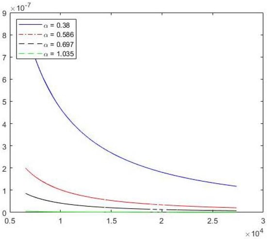
Figure 3. The shape of the tails of the $S\&P500$ daily data at various alpha values (see Table 1) with $\eta =0,m=0$ and $\sigma =1$, shows that the data has a heavier tail when $\alpha$ decreases.

Table 1. Estimating the value of $\alpha$ at various $\gamma$ values in the range $(0,1)$ while fitting to real market data (DJIA, $S\&P500$, and TASI).

Estimating the Value of Alpha
Index	$\gamma$	0.3	0.5	0.6	0.7	0.9
DJIA	$\alpha$	0.298	0.459	0.634	0.441	0.809
S&P 500	$\alpha$	0.38	0.586	0.697	0.810	1.035
Tasi	$\alpha$	0.299	0.452	0.535	0.62	0.796

Figure 4, Figure 5 and Figure 6 refer to the calculation of the entropy analysis for different values of gamma from different stock markets (DJIA, $S\&P500$, and TASI). We demonstrate that the scaling behavior of different indices is almost the same, with the gamma values in the interval (0,1). Figure 4 presents the results for entropy analysis of (34) and the solution (37) at a series of times for the DJIA, which show the values of $\alpha$ = $0.298,0.459,0.634,0.441$ and $0.809$ for five different values of $\gamma$ ($\gamma$ = 0.3, 0.5, 0.6, 0.7, and 0.9, respectively). Based on $\gamma$, there is a distinct monotonic relationship where the entropy increases when $\alpha$ decreases.

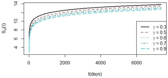
Figure 4. The entropy analysis for the DJIA at different values of $\gamma$ when $\alpha$ = 0.298, 0.459, 0.634, 0.441 and 0.809, based on gamma, there is a distinct monotonic relationship where the entropy increases when alpha decreases.

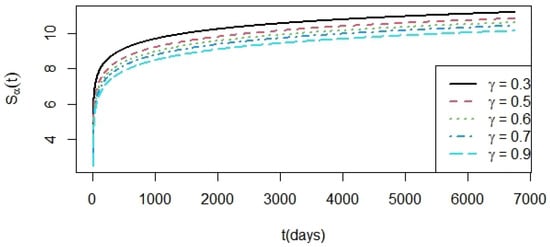
Figure 5. The entropy fractional time analysis for $S\&P500$ at varying $\gamma$ between 0 and 1, where $\alpha$ = 0.38, 0.586, 0.697, 0.810, and 1.035, from Table 1, the monotonic increase of $\alpha$ for increasing $\gamma$ is accompanied by the monotonic decrease of $S(P,t)$ for increasing, demonstrating the regime’s $\alpha$ ordering.

Figure 6. The entropy analysis of (34) for the TASI, where $\alpha$ = 0.299, 0.452, 0.535, 0.62, and 0.796 from Table 1, the monotonic increase of $\alpha$ for increasing $\gamma$ is accompanied by the monotonic decrease of $S(P,t)$ for increasing, demonstrating the regime’s $\alpha$ ordering.

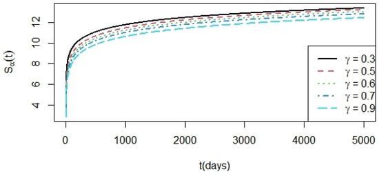
Figure 5 shows the results of the entropy analysis of (34) and the solution (37) for the S&P 500 index daily data series time; this shows the values of $\alpha$ in Table 1 for five different values of $\gamma$ between 0 and 1.

The next figure, Figure 6 shows the results of the entropy analysis of (34) and the solution (37) for the (TASI) index daily data series time, where $\alpha$ as presented in Table 1 for five different values of $\gamma$ of $0.3,0.5,0.6,0.7$ and $0.9$.

Figure 7, Figure 8 and Figure 9 calculate the entropy for different values of $\gamma$ fitting to GBP/USD, USD/SAR, and USD/JYP real-market exchange rates from 2000 to 2022. Figure 7 depicts the results of the entropy analysis (34) of the GBP/USD exchange rate, with the $\alpha$ fitting the values ($0.698,1.091,1.31,1.505$, and $1.866$) from Table 2.

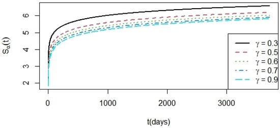
Figure 7. The entropy analysis for the GBP/USD exchange rate from 2000 to 2022 has an harmonic inverse relation with the $\alpha$ values ($0.698,1.091,1.31,1.505$, and $1.866$)from Table 2, for some $\gamma$ values between 0 and 1.

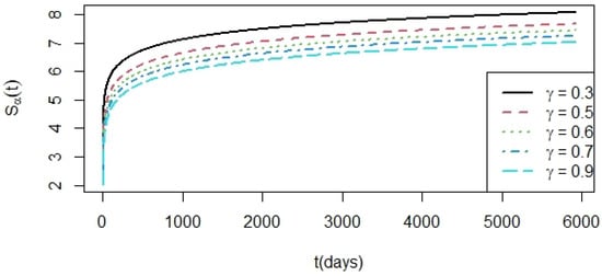
Figure 8. The entropy analysis fitting the USD/JPY exchange rate 2000 to 2022 has a harmonic inverse relation of the $\alpha =0.56,0.875,1.049,1.225$ and $1.565$ from Table 2 which are estimated for some values of $\gamma \in (0,1)$.

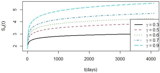
Figure 9. The entropy analysis for fitting the real data market USD/SAR exchange rate, where $\alpha =1.99$ for all $\gamma$ values in the interval $(0,1)$; when $\alpha$ is close to 2, it indicates that the exchange rate of USD/SAR has a normal distribution.

Table 2. Estimating the value of $\alpha$ at various $\gamma$ values in the range $(0,1)$ while fitting to GBP/USD, USD/SAR, and USD/JYP real market exchange rates from 2000 to 2022.

Estimating the Value of Alpha
Index	$\gamma$	0.3	0.5	0.6	0.7	0.9
GBP/USD	$\alpha$	0.698	1.091	1.31	1.505	1.866
USD/SAR	$\alpha$	1.99	1.99	1.99	1.99	1.99
USD/JPY	$\alpha$	0.56	0.875	1.049	1.225	1.565

The next figure, Figure 8 shows the results for the entropy analysis (34) of the exchange rate of USD/JPY, where the $\alpha$ is fitting the values ($0.56,0.875,1.049,1.225$ and $1.565$) from Table 2.

We depicted the results in Figure 9 of the entropy analysis to fit the real market USD/SAR exchange rate, with an estimated alpha for any $\gamma$ value in $(0,1)$ yielding $\alpha =1.99$. The USD/SAR exchange rate follows a normal distribution if $\alpha$ is close to 2.

6. Conclusions

In this study, the fractional time–space Fokker–Planck equation is driven by the Lévy fractional time diffusion model. When $\eta =0$, an analytical solution to the fractional Fokker–Planck equation of the Caputo time derivative of order $0<\gamma <1$ and Riemann–Liouville fractional space derivative $0<\alpha <2$ is calculated and represented using the Fox representation. As a result, the calculation above demonstrates how the entropy production rate $R(t)$ depends on the fractional orders of space and time, $\alpha$ and $\gamma$, respectively. The entropy production rate of the traditional one-dimensional diffusion equation and the fractional space one-dimensional equation in [32], which do not depend on order, are different from the entropy production rate of the fractional time-space Fokker–Planck equation, which depends on orders. When $\alpha$ decreases, the heavier tails in the stock markets (DJIA, TASI, and $S\&P500$) increase. Moreover, in the exchange rates of GBP/USD and USD/JYP, when the $\gamma$ is close to 1, then the $\alpha$ is close to 2. In addition, the USD/SAR exchange rate $\alpha$ is approximately 2 at any value of $\gamma$ (approximate normal distribution); see Table 2.

References

- Millar, K.S.; Ross, B. An Introduction to the Fractional Calculus and Fractional Differential Equations; Wiley: New York, NY, USA, 1993. [Google Scholar]
- Podlubny, I. Fractional Differential Equations; Academic Press: San Diego, CA, USA, 1998. [Google Scholar]
- Hoffmann, K.H.; Essex, C.; Schulzky, C. Fractional diffusion and entropy production. J. Non-Equilib. Thermodyn. 1998, 23, 166–175. [Google Scholar] [CrossRef]
- Mainardi, F.; Pagnini, G.; Saxena, R.K. Fox H functions in fractional diffusion. J. Comput. Appl. Math. 2005, 1, 321–331. [Google Scholar] [CrossRef]
- Aljedhi, R.A.; Kılıçman, A. Fractional Partial Differential Equations Associated with Lévy Stable Process. Mathematics 2020, 4, 508. [Google Scholar] [CrossRef]
- Aljedhi, R.A.; Kılıçman, A. Financial Applications on Fractional Lévy Stochastic Processes. Fractal Fract. 2022, 5, 278. [Google Scholar] [CrossRef]
- Duan, J.S.; Yanovsky, V.V.; Lovejoy, S. Fractional Fokker–Planck equation for nonlinear stochastic differential equations driven by non Gaussian Lévy stable noises. J. Math. Phys. 2001, 24, 200–212. [Google Scholar]
- Yanovsky, V.V.; Chechkin, A.V.; Schertzer, D.; Tur, A.V. Lévy anomalous diffusion and fractional Fokker–Planck equation. J. Math. Phys. 2001, 1, 13–34. [Google Scholar] [CrossRef]
- Essex, C.; Hoffmann, K.H.; Davison, M. Fractional diffusion, irreversibility and entropy. J. Non-Equilib. Thermodyn. 2016, 24, 279–291. [Google Scholar]
- Prehl, J.; Essex, C.; Hoffmann, K.H. The superdiffusion entropy production paradox in the space-fractional case for extended entropies. Phys. A Stat. Mech. Its Appl. 2010, 2, 214–224. [Google Scholar] [CrossRef]
- Lewis, A.L. A Simple Option Formula for General Jump-Diffusion and Other Exponential Lévy Processes; Working Paper; Envision Financial Systems: Newport Beach, CA, USA, 2001. [Google Scholar]
- Alvaro, C.; del-Castillo-Negrete, D. Fractional Diffusion Models of Option Prices in Markets with Jumps. Stat. Mech. Its Appl. 2007, 2, 749–763. [Google Scholar]
- Benson, A.; Schumer, R.; Meerschaert, M.; Wheatcraft, W. Fractional Dispersion, Lévy Motion, and the MADE Tracer Tests. Transp. Porous Media 2001, 1, 211–240. [Google Scholar] [CrossRef]
- Metzler, R.; Barkai, E.; Klafter, J. Deriving fractional Fokker-Planck equations from a generalised master equation. Europhys. Lett. 1999, 4, 431–436. [Google Scholar] [CrossRef]
- Oppenheim, I.; Shuler, K.E.; Weiss, G.H. Stochastic Processes in Chemical Physics: The Master Equation; The MIT Press: Cambridge, MA, USA, 1977. [Google Scholar]
- Jumarie, G. Derivation and solutions of some farctional Black-Scholes equations in space and time. J. Comput. Math. Appl. 2010, 3, 1142–1164. [Google Scholar] [CrossRef]
- Kenkre, V.M. Generalized Master Equations Under Delocalized Initial Conditions. J. Stat. Phys. 1978, 4, 333–340. [Google Scholar] [CrossRef]
- Meerschaert, M.M.; Tadjeran, C. Finite difference approximations for fractional advection-dispersion flow equations. J. Comput. Appl. Math. 2004, 1, 65–77. [Google Scholar] [CrossRef]
- Merton, R. Continuous-Time Finance, 1st ed.; Basil Blackwell: Oxford, UK, 1990. [Google Scholar]
- Schoutens, W. Lévy Processes in Finance. Wiley Series in Probability and Statistics, 1st ed.; Wiley: Oxford, UK, 2003. [Google Scholar]
- Zhang, Y. A finite difference method for fractional partial differential equation. J. Comput. Appl. Math. 2009, 2, 524–529. [Google Scholar] [CrossRef]
- Knopova, V.; Kulik, A. Exact asymptotic for distribution densities of Lévy functional. J. URL 2011, 52, 1394–1433. [Google Scholar] [CrossRef]
- Pielaszkiewicz, J.; von Rosen, D.; Singull, M. Cumulant-moment relation in free probability theory. Acta Comment. Univ. Tartu. Math. 2014, 2, 265–278. [Google Scholar]
- Luchko, Y.F.; Matrínez, H.; Trujillo, J.J. Fractional Fourier transform and some of its applications. J. Fract. Calc. Appl. Anal. 2008, 4, 457–470. [Google Scholar]
- Janett, P.; Frank, B.; Karl, H.-H.; Christopher, E. Symmetric Fractional Diffusion and Entropy Production. Entropy 2016, 7, 275. [Google Scholar] [CrossRef]
- Saichev, A.I.; Zaslavsky, G.M. Fractional Kinetic Equations: Solutions and Applications. Chaos 1997, 1, 753–764. [Google Scholar] [CrossRef]
- Duan, J.S.; Chaolu, T.; Wang, Z.; Fu, S.Z. Lévy stable distribution and space-fractional Fokker-Planck type equation. J. King Saud Univ. 2016, 24, 17–20. [Google Scholar] [CrossRef]
- Demirci, E.; Ozalp, N. A method for solving differential equations of fractional order. J. Comput. Appl. Math. 2012, 11, 2754–2762. [Google Scholar] [CrossRef]
- Duan, J.S. Time- and space-fractional partial differential equations. J. Math. Phys. 2005, 1, 13504–13511. [Google Scholar] [CrossRef]
- Glöckle, W.G.; Nonnenmacher, T.F. Fox function representation of Non-Debye relaxation processes. J. Stat. Phys. 1993, 3, 741–757. [Google Scholar] [CrossRef]
- Mainardi, A.M.; Saxena, R.K. The H Function with Applications in Statistics and Other Discplines; Wiley Eastern: New Delhi, India; Willey Halsted: New York, NY, USA, 1978. [Google Scholar]
- Luchko, Y. Entropy Production Rate of a One-Dimensional Alpha-Fractional Diffusion Process. Axioms 2016, 1, 6. [Google Scholar] [CrossRef]
- Mathai, A.M.; Haubold, H.J.; Saxena, R.K. The H Functions Theory and Applications; Springer: New York, NY, USA, 2010. [Google Scholar]
- Palatella, L.; Montero, M.; Perelló, J.; Masoliver, J. Diffusion Entropy technique applied to the study of the market activity. Phys. A Stat. Mech. Its Appl. 2005, 1, 131–137. [Google Scholar] [CrossRef]
Disclaimer/Publisher’s Note: The statements, opinions and data contained in all publications are solely those of the individual author(s) and contributor(s) and not of MDPI and/or the editor(s). MDPI and/or the editor(s) disclaim responsibility for any injury to people or property resulting from any ideas, methods, instructions or products referred to in the content. |
© 2023 by the authors. Licensee MDPI, Basel, Switzerland. This article is an open access article distributed under the terms and conditions of the Creative Commons Attribution (CC BY) license (https://creativecommons.org/licenses/by/4.0/).