Abstract
The contemporary scientific community is very familiar with implicit block techniques for solving initial value problems in ordinary differential equations. This is due to the fact that these techniques are cost effective, consistent and stable, and they typically converge quickly when applied to solve particularly stiff models. These aspects of block techniques are the key motivations for the one-step optimized block technique with two off-grid points that was developed in the current research project. Based on collocation points, a family of block techniques can be devised, and it is shown that an optimal member of the family can be picked up from the leading term of the local truncation error. The theoretical analysis is taken into consideration, and some of the concepts that are looked at are the order of convergence, consistency, zero-stability, linear stability, order stars, and the local truncation error. Through the use of numerical simulations of models from epidemiology, it was demonstrated that the technique is superior to the numerous existing methodologies that share comparable characteristics. For numerical simulation, a number of models from different areas of medical science were taken into account. These include the SIR model from epidemiology, the ventricular arrhythmia model from the pharmacy, the biomass transfer model from plants, and a few more.
Keywords:
collocation; implicit block; relative stability; convergence; mathematical epidemiology; numerical simulations MSC:
65L05; 65L20
1. Introduction
In this study, we focus on finding numerically close solutions to first-order initial-value problems (IVPs) for ordinary differential equations (ODEs) of the type
where d is the dimension of the system. With an initial value of and a continuous function f that meets Lipchitz’s condition, we can check that the existence and uniqueness theorem holds for this problem (see [1]). The numerical value of the theoretical solution at is denoted by . In order to obtain a theoretical solution to ODEs in a computationally efficient manner, numerical methods are necessary [2,3] because they may be used to describe physical events, such as the movement of objects in space or the flow of liquids through pipes. ODEs find extensive applications in the fields of engineering, physics, logistic damping effect in chemotaxis models, epidemiology, applied microbiology and biotechnology [4,5,6,7]. In this way, numerical approaches give us the tools we need to solve ODEs quickly and accurately. The primary advantage of numerical methods is that they provide solutions to ODEs that may be implemented rapidly and without the requirement for integration over extended periods of time. Because numerical approaches can account for the effects of a variable’s values over time, they are often more accurate than analytical methods. In general, numerical approaches are crucial for solving ODEs because they permit more rapid and precise solution derivation. Engineers and scientists can examine the behavior of a system in many scenarios much more rapidly and precisely when they use numerical approaches [8,9].
It is of the utmost importance to develop numerical approaches that are both exact and efficient for tackling the challenges that are related to ordinary differential equations. This is due to the fact that ordinary differential equations find widespread applicability in the current world. In this particular setting, the body of previous research provides a variety of distinct numerical methods as viable answers to the problem at hand. Many different domains, including chemistry, flame propagation, computational fluid dynamics, population dynamics, engineering, microbiology and mathematical biology, require approximate solutions to challenging issues; nevertheless, the bulk of available numerical methods do not meet the requirements. In order for models to have adequate rigidity in terms of having non-linearity and stiffness, numerical methods that are not only computationally expensive but also need to have unbounded stability areas must be used [10,11].
One of the main weaknesses of numerical methods for solving ODEs is that they can be computationally expensive. Numerical methods require the use of large amounts of data to create a solution, and this requires a significant amount of computing power and time to calculate. Additionally, numerical methods can be inaccurate if the data used are not precise enough or if the steps taken in the numerical solution are too small. Another limitation of numerical methods is that they typically rely on approximations of the true solution, and this can lead to inaccuracies in the results. Additionally, numerical methods can produce a limited number of solutions, as they are often designed to solve specific types of ODEs. Finally, numerical methods can be difficult to debug and modify, as they involve complex algorithms and equations. Overall, numerical methods for solving differential equations have their strengths and weaknesses, and it is important to consider both when deciding which method to use. With careful consideration and proper implementation, numerical methods can provide accurate and efficient solutions to ODEs [12].
Due to high computing cost (extremely tiny step size ) or limited stability region, most conventional methods, such as explicit Runge–Kutta, the Lobatto family, the multi-step Adams family, and higher-order multi-derivative types, are not employed. However, the implicit block procedures are recommended since they can begin by themselves, are computationally robust (cheap), are extremely accurate, converge quickly, and are mathematically stable (with or stability features). The most significant advantages of block approaches are their ability to initiate themselves and prevent overlapping between different parts of solutions. However, the stability areas of some block approaches are extremely small, and that is a drawback of the methodology suggested here [13,14]. In future research work, this shortcoming will be removed.
By applying multiple formulas to the IVP at once, as in the block strategy, they are able to improve upon one another and provide a more accurate estimate. ODEs of the form (1) have been tackled using block methods in a number of publications [15,16], and there are block methods with several features for tackling higher-order problems as described in [17,18]. Modern computer algebra systems (CASs), such as MAPLE and MATHEMATICA, provide a plethora of pre-built numerical code functions that simplify the process of getting numerical approximations to the theoretical solution. These programs are optimized for solving problems with variable step sizes that can have a wide variety of solutions, including those that are stiff, non-stiff, singular, etc. Due to the numerical instability of some numerical approaches, stiff systems are among the most difficult systems to solve. Notable academics have expended a lot of effort to develop more effective means of addressing such problems. There are already numerical approaches for solving (1), but utilizing a variable step-size formulation with an appropriate error estimation can increase the accuracy and rate of convergence. In this study, we also aim to find a new one-step way to find the approximate solution to first-order IVPs of the type given in (1), using both fixed and adaptive step-size formulations.
The remaining sections of the paper are as follows: The next part (Section 2) of the present article will discuss the new technique’s creation. In Section 3, we analyze the proposed procedure. The suggested technique’s adaptive step-size formulation is described in Section 4, and its implementation is covered in Section 4.1. In Section 5, we provide several real-world examples drawn from the natural sciences to demonstrate the effectiveness and accuracy of the proposed approach. Finally, a brief conclusion is provided in Section 6, which also includes suggestions for moving forward.
2. Mathematical Formulation
In this part, we derive the one-step optimized block method with two off-grid points, while considering in (1) to facilitate the derivation. The off-grid points are optimized by using the main formula’s local truncation error denoted by . Let us take into consideration the partition on the integration interval , with constant step-length , . Taking this into consideration, we assume an approximation to the theoretical solution of (1) by an appropriate interpolating polynomial of the form as given below:
where represent real unknown parameters. Differentiating (2) with respect to x, one obtains
Take into consideration the two off-grid points as and with in order to calculate the estimated solution of the IVP (1) at the point under the assumption that . It is crucial to note at this point that the local truncation error of the main formula will be used to compute the optimal values of these two off-grid points. Consider that the polynomial in (2) and its first derivative in (3) are evaluated at the point , while the second derivative of in (4) is evaluated at the points as follows:
This above setting results in a system of five equations with five real unknown parameters . These equations can be arranged in matrix form as follows:
The five unknown coefficients (), which are computed by solving the above linear system, are not, for the sake of conciseness, shown here. However, substituting the values of these five parameters in (2) while utilizing the variable change , we reach the following:
where,
We examine the one-step block approach to obtain at the collocation points , and . In (6), we take . The resulting three formulas are as follows:
where are approximations of the true solution , and for . The aforementioned approximations use two unknown parameters and two off-grid points . We set the first two terms of the local truncation error from (10) to zero to acquire suitable values for these parameters (u and v). By doing so, optimal parameters will be acquired, and at the end of the generic subinterval , the only value needed to advance the integration is . Taylor expansion allows us to calculate the following local truncation error () of the main formula given in (10):
The coefficients of and are equated to zero and the following optimal values of the parameters (u and v) are obtained from the resulting algebraic system, as is similar to what occurs while utilizing numerous other approaches to solving with numerical solutions of partial differential equations (see [19,20]):
Substituting the above optimal values into the local truncation errors of the formulae (8) to (10), we obtain the following:
Putting the optimal values given in (12) into formulae (8) to (10), the following one-step optimized block method with two off-grid points is produced, whereas the pseudo-code for the method (fixed stepsize) is provided in Algorithm 1.
| Algorithm 1: Pseudo-code for the optimized hybrid block technique with two intra-step points with a fixed stepsize approach. |
| Data: (integration interval), N (number of steps), , |
| (initial values), |
| Result: sol (discrete approximate solution of the IVP (1)) |
| 1 Let |
| 2 Let |
| 3 Let sol |
| 4 Solve (14) to get where |
| 5 Let sol = sol |
| 6 Let |
| 7 Let |
| 8 if then |
| 9 go to 13 |
| 10 else |
| 11 go to 4; |
| 12 end |
| 13 End |
3. Theoretical Analysis
In this section, we offer an examination of the fundamental properties of the one-step optimized block approach that was presented in the aforementioned section. These fundamental qualities include the following: order of convergence, zero-stability, linear stability, consistency, and relative measure of stability.
3.1. Order of Convergence
Rewritten using the matrix notation, for are introduced to augment the zero entries of the vector notations. Thus, the new proposed optimal block method abbreviated as NPOBM in the matrix form is given below:
where and are matrices given by
The proposed method is formulated from the Equation (14) by defining the vectors , and as follows:
3.2. Accuracy and Consistency
Following the procedure in [21] and assuming that is a sufficiently differentiable function, we define the operator given as follows:
where and . By utilizing the Taylor series about , we expand the formula in Equation (19) and obtain the following identity:
Following the guidelines given in [22], Equation (20) and the associated formulas are said to be of algebraic order r if where is the coefficient of the power in the Taylor series expansion of (19). The proposed approach developed in (14) has , and
Thus, each formula in the new proposed optimized block method (NPOBM) has at least a fourth algebraic order of convergence. It should be noted that this gives a lower constraint to the order. In order to obtain the correct order, the suggested approach can be reformulated as an RK method [23]; in reality, the theory of RK methods will offer the method’s order, which is six. We demonstrate that this result is consistent with the numerical data in Section 5. Since the proposed method has an order higher than one, thus, based on [24], it is consistent.
3.3. Zero Stability and Convergence
A numerical method for IVPs is called zero-stable if it maintains the stability of the trivial solution (i.e., the solution where all variables are equal to zero) as the solution is advanced in time. This means that any small perturbations in the initial conditions will remain small as the solution is calculated, and will not grow or cause the solution to become unbounded. Zero stability is an important property for numerical methods, as it helps ensure that the method will produce meaningful results, even when the initial conditions are only known approximately. The stability of a numerical method can be assessed through the use of stability analyses, such as the von Neumann stability analysis, or by running the method on test problems and examining the behavior of the solution. If a numerical method is not zero-stable, it may produce solutions that diverge from the true solution, or become unbounded, as the solution is calculated. In such cases, the method may be considered unreliable and may need to be improved or modified in order to produce more accurate results.
In this section, we demonstrate the stability of the suggested one-step optimized block strategy with two off-grid points and we also discuss the convergence of the proposed method. The concept of zero-stability relates to considering a homogeneous equation and its discretized version, as written below:
where is the the matrix that was shown previously in Section 3.1, whereas is a identity matrix. Now, if the discrete algebraic Equation (21) allows solutions that develop in time, then the suggested block technique will not be zero-stable and thus not be of any use. On the contrary, if the zeros of the first characteristic polynomial fulfills and for those zeros with , the multiplicity should not exceed 1 as stated in [25]. The first characteristic polynomial of the proposed block method (14) is given by
3.4. Linear Stability Analysis
The concept of linear stability is particularly important in the study of dynamical systems, where it is used to determine the long-term behavior of a system and to identify critical points that determine the stability of the system. It is also used in control theory to design controllers that stabilize unstable systems, and in engineering and physics to study the stability of structures and fluid flows. The step-length characterizes the behavior of the underlying numerical technique. This behavior is connected to the idea of zero stability, which is related to the behavior of the method. In other situations though, a practical point of view requires a different idea of stability. To be stable, a numerical method must be able to reliably give results for some non-zero value of the step-length, denoted here by notation . For the numerical approach that is being considered, this kind of behavior is referred to as the linear stability behavior, and it involves applying the strategy described by Dahlquist [27] for solving a linear test problem and is provided by
It is necessary to find the area of the linear test problem presented in (23), within which the approximations generated using the numerical technique replicate the behavior of the precise solution to the issue. When the optimized block approach from (14) is used to solve the linear test problem from (23), the following recurrence equation is found:
where is the stability matrix defined by
By substituting matrices given in Section 3.1 into Equation (16), the spectral radius is now obtained:
The behavior of the approximate numerical solution is determined by the eigenvalues of the stability matrix, which is denoted by the notation given in Equation (16). This is a characteristic of a numerical method that makes use of the spectral radius. This is a property that is well known and widely used in practice as in [28]. The following set may be used to provide a description of the area of absolute linear stability denoted by :
The visual explanations in Figure 1 demonstrate that some part of the complex plane, denoted by , is contained in the stability region of the optimized block method in (14) that is said to be conditionally stable if some part of .
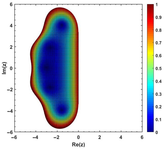
Figure 1.
Stability region (shaded region) obtained from Equation (26) for the proposed optimal block technique.
3.5. Relative Measure of Stability
The relative measure of stability, which is commonly called the order star, is an effective and strong contemporary technique for numerical approaches. It gives essential information, such as order and stability considerations, for the numerical approach that is being used within the context of a framework that is consistent. With regard to the approach of the conditional stable block method (14), we have ; this is provided by an approximation that can be rationalized. Additional appealing characteristics are associated with this form of approximation. Investigating the characteristics of a relative approximation in the complex plane may be performed with the assistance of an order star. It is essential to keep in mind that our interest in numerical methods usually gives origin to our interest in the study of qualities that are approximations.
Let and be possibly complex-valued polynomials of degree m and n, respectively, and denote the quotient by . Certainly, a zero of is a pole of the rational function . Let be a complex function. An order star defines a partition in the complex plane, namely the triplet , where
Fundamentally, there are two types of order stars, , that are usually considered in the literature as follows:
Some of the properties related to the order stars are stated below:
Property 1
(Order). is an order q approximation to if z is connected by parts of and divided by parts of . With an asymptotic angle of , all parts approach z. Bounded, related parts of are commonly referred to as fingers, whereas similar sections of are referred to as dual fingers.
Property 2
(Enumeration). The number of poles (zeros) in each bounded linked part of , multiplied by their multiplicity, equals the number of interpolation points (i.e., such that = .
Property 3
(Unbounded). There are two unbounded associated parts, one of and the other of .
It is standard practice to shade the former in order to identify it from the latter, which is written as . When this is done, it is made abundantly evident that the zone of growth of relative stability is indicated for the set that is symbolized by , while the region of counter activity falls within the set that is designated by . As a direct consequence of this, the variable is used to establish the limit between the area of relative stability and the region of contractility. By redefining the order star of , one may create a set consisting of the following three regions, which can then be taken into consideration. Because the first kind of order star is of the utmost importance to us, we determined the following sets to be true:
The graphs of the above sets yield some star-like (fingers) different from the one we are familiar with (regions of absolute stability). These fingers are shown in Figure 2.
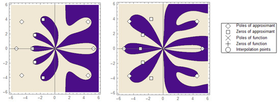
Figure 2.
The plot of order stars of the first kind (right) and the order stars of the second kind (left) using the proposed one-step optimized block technique presented in Equation (14).
4. Adaptive Stepsize Approach
In this section, we present an adaptive step-size formulation for the one-step optimal approach that was given earlier. This will make it possible for us to obtain an effective formulation that will supply accurate numerical approximations to the IVP, as we will see in the following section. In the introduction, it is mentioned that in order to make efficient use of numerical methods, one must adjust the step size according to the way the solution behaves locally. An embedding strategy is typically used for this purpose, which means that in addition to the approximation for , an additional lower-order technique must be obtained to estimate the local error (LE) at the final point of each integration step. This is because the approximation for is a higher-order technique. The estimate of the LE can be found by taking the difference between the two approximations. For the considered second-order explicit method given in [29], this choice does not cost any additional computational burden while simulating the differential systems:
and the local truncation error, LTE, is employed to estimate the local error through the following difference equation:
If , where TOL stands for the tolerance predefined by the user, then this is the point where we agree with the results and select the next step as , to minimize the computational burden and continue the integration process with with the assumption that . However, if , then we need to reject the achieved results by reducing them and repeating the calculations with the new step as follows:
Here, the order of the lower-order technique (32) is denoted by the value , while the value denotes a safety factor whose purpose is to circumvent the steps that were unsuccessful. In the part devoted to numerical examples, we took into consideration both a very modest initial step size as well as a strategy for modifying the step size that, if required, will cause the algorithm to alter the step size. Algorithm 2, in the form of pseudo-code, explains the implementation of the adaptive stepsize version of the proposed optimized block method.
| Algorithm 2: Pseudo-code for the two-step optimized hybrid block method with two intra-step points under variable stepsize approach. |
Data: Initial stepsize: , ; Integration interval: ; Initial value: ; Function f: ; Given tolerance: TOL Result: Approximations of the problem (1) at selected points. 1 if then 2 end 3 if then 4 end 5 while , then solve system of equations in (14) to get the values do 6 compute to get EST. 7 end 8 if TOL then accept the results and substitute then 9 end 10 Set , and use the formula in (32) to determine the new stepsize. 11 if TOL, then reject the results and repeat the calculations using (32) and go to step (6) then 12 end 13 end |
4.1. Implementation Steps
The proposed method NPOBM given in (14) is implicit, which means that on each step, a system of equations must be solved. Those systems, which provide the values at each step, are usually solved using Newton’s method or its variants. Here, we adopted in the numerical realization of the scheme the solution provided by the command FindRoot in Mathematica , which uses a Newton damped method. As it is well known, this kind of procedure presents local convergence, which means that good starting values must be provided. In what follows, we summarize below how NPOBM is applied to solve IVPs.
- Step 1. Choose N, , on the partition .
- Step 3. Next, for , the values of and are simultaneously obtained over the sub-interval , as and are known from the previous block.
- Step 4. The process is continued for to obtain the numerical solution to (1) on the sub-intervals .
5. Biological Models for Numerical Simulations
This section discusses the numerical simulations of the proposed block method given in (14) on the basis of accuracy via error distributions (absolute maximum global error , absolute error computed at the last mesh point over the chosen integration interval , norm , and root mean square error , precision factor (scd ), and time efficiency (CPU time measured in seconds). In order to acquire after successfully solving the system, we took advantage of the well-known and widely used second-order convergent Newton–Raphson approach. The next step in the process involves determining the value by using the value . As the starting value, we use the value from the preceding block. This process is repeated until the destination point () is reached. We determined that the length of the integration interval is because the suggested methodology is a one-step method and some of the methods used for comparisons are one- and two-step. The Newton–Raphson method was implemented using the FindRoot command, which is provided in Mathematica . It is important to mention that all of the numerical calculations are carried out using Mathematica , which is installed on a personal computer that is powered by Windows OS and has an Intel(R) Core(TM) i7-1065G7 CPU @ 1.30GHz 1.50GHz processor with 24.0 GB of installed RAM. It is also worth noting that we employed one sixth-order approach and two, at least, fifth-order ones for the purpose of comparison. Included are the following methods for the numerical comparative analysis:
- NPOBM: New proposed optimal block method given in (14).
- MHIRK: Multi-derivative hybrid implicit Runge–Kutta method with fifth-order convergence, which appeared in [30].
- RADIIA and IRK: Fully implicit RK-type fifth-order methods, which appeared in [31]
- Sahi: -stable hybrid block method of order six, which appeared in [32].
- LPHBM: Laguerre polynomial hybrid block method of sixth-order convergence, which appeared in [33].
Different kinds of biological models based on differential equations are taken into consideration to analyze the performance of the proposed block technique presented in Equation (14). For the numerical simulations, the following notations were used:
- : step-size.
- : initial step-size.
- LE: local error estimate.
- LTE: Local truncation error.
- MaxErr: Maximum error on the selected grid points over the chosen integration interval.
- RMSE: Root mean square error on the selected grid points over the chosen integration interval.
- FFE: Total number of function evaluations.
- NS: Total number of steps.
- TOL: Predefined tolerance.
- CPU: Computational time in seconds.
Problem 1

(Susceptible–Infected–Recovered (SIR) Model [34]). The SIR model is an epidemiological model that computes the theoretical number of people infected with an infectious illness in a closed community over the course of time. This number is based on the assumption that the disease spreads from person to person. This category of models gets its name from the fact that they use coupled equations to relate the numbers of sensitive individuals to one another. The total number of susceptible people is , the total number of infected people is , and the total number of people who have recovered is . This is a useful and simple way to explain a wide range of diseases that spread from person to person. Included are diseases such as measles, mumps, and rubella that can be explained via this well-known model. The flowchart of the model is given in Figure 3.
Figure 3.
Flow chart of the SIR model.
The nonlinear differential system describing the SIR model is shown below:
where and are positive parameters. Define to be:
By adding all equations in (33), we obtain
Taking into consideration with initial condition , the exact solution is as follows: . The SIR model is simulated with different techniques, and the results are tabulated. Both constant and adaptive stepsize approaches are used. It can be seen in Table 1, Table 2 and Table 3 that the proposed technique (14) not only yields the minimum errors, but it also goes with the highest scd factor, thereby proving the much better performance of (14) in comparison to other well-known block techniques. In addition, the superiority of the proposed technique is maintained, even when the adaptive stepsize approach is utilized with varying values of the tolerance as shown in Table 4. Finally, the efficiency curves produced with each technique under consideration speak volumes in favor of (14) since they take the shortest time to yield the smallest maximum absolute global error as shown in Figure 4.

Table 1.
Numerical results for Problem 1 with NS = , where .
Table 2.
Numerical results for Problem 1 with NS = where .
Table 3.
Numerical results for Problem 1 with NS = where .
Table 4.
Numerical results for Problem 1 with adaptive step-size approach while .
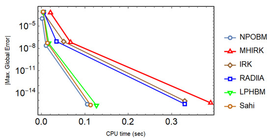
Figure 4.
Efficiency curves for the system in Problem 1 to observe the behavior of absolute maximum global errors versus the CPU time (sec) with a logarithmic scale on y-axis.
Problem 2

(Application on Irregular Heartbeats and Lidocaine model [35]). Clinically, the condition known as ventricular arrhythmia, also known as an irregular heartbeat, may be treated with the medication lidocaine. The medicine must be kept at a bloodstream concentration of 1.5 milligram per liter in order for it to be effective. However, concentrations of the drug in circulation that are over 6 milligram per liter are believed to be deadly in certain people. The exact dose is determined by the body weight of the patient. It has been stated that the highest adult dose for ventricular tachycardia is 3 milligrams per kilogram. The medicine comes in 0.5%, 1%, and 2% concentration solutions that can be kept at room temperature. A model based on differential equations that captures the dynamic nature of pharmacological treatment was designed in [36], whose flowchart (Figure 5) is given as follows:
Figure 5.
Xylocaine label, brand name of the drug lidocaine [36].
The set of linear equations describing the above phenomenon is given as follows:
The physically significant initial data are zero drug in the bloodstream and the injection dosage is . The exact solution for IVP given in (36) is computed as follows:
The irregular heartbeats and lidocaine model is simulated with different techniques, and the results are tabulated. Both constant and adaptive stepsize approaches are used. It can be seen in Table 5, Table 6 and Table 7 that the proposed technique (14) not only yields minimal errors, but it also goes with the highest scd factor, thereby proving the much better performance of (14) in comparison to other well-known block techniques. In addition, the superiority of the proposed technique is maintained, even when the adaptive stepsize approach is utilized with varying values of the tolerance as shown in Table 8. Finally, the efficiency curves produced with each technique under consideration speak volumes in favor of (14) since they take the shortest time to yield the smallest maximum absolute global error as shown in Figure 6.
Table 5.
Numerical results for Problem 2 with NS = where .
Table 6.
Numerical results for Problem 2 with NS = where .
Table 7.
Numerical results for Problem 2 with NS = where .
Table 8.
Numerical results for Problem 2 with adaptive step-size approach while .
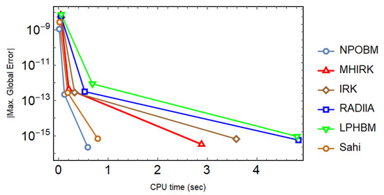
Figure 6.
Efficiency curves for the system in Problem 2 to observe the behavior of absolute maximum global errors versus the CPU time (sec) with a logarithmic scale on y-axis.
Problem 3
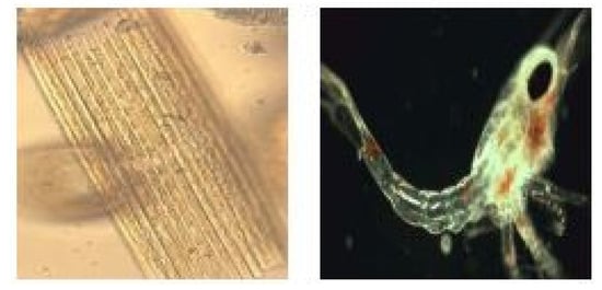
(Nutrient Flow in an Aquarium [37]). This flow is important for maintaining a healthy and balanced aquatic environment, as it supports the growth and survival of plants and animals in the aquarium. Imagine there is a body of water that has a radioactive isotope that is going to be utilized as a tracer for the food chain. The food chain is made up of several types of aquatic plankton, such as A and B. Plankton are defined as creatures that live in water and move with the flow of the water, and may be found in such places as the Chesapeake Bay. There are two different kinds of plankton, which are known as phytoplankton and zooplankton. The phytoplankton are plant-like organisms that float across the water, including diatoms and other types of algae. Animal-like organisms that float in the water known as zooplankton include copepods, larvae, and small crustaceans. Figure 7 explains the phenomenon.
Figure 7.
(Left): Bacillaria paxillifera, phytoplankton. (Right): Anomura Galathea zoea, zooplankton.
More complex models might consider additional factors, such as the interactions between different types of plants and animals, the effects of different types of filtration systems, and the influence of water temperature and light intensity on the rate of photosynthesis. By considering these relationships, a differential equation model can provide a more comprehensive description of the nutrient flow in an aquarium and help to understand how changes in one aspect of the system might affect other parts of the system. The state variables are explained as follows: represents the concentration of an isotope in the water; represents the concentration of an isotope in A; and represents the concentration of an isotope in B. They are used in the following coupled linear system of differential equations:
with initial condition is , and . The exact solution is as follows:
Model (37) is simulated with different techniques, and the results are tabulated. Both constant and adaptive stepsize approaches are used. It can be seen in Table 9, Table 10 and Table 11 that the proposed technique (14) not only yields the minimum errors, but it also goes with the highest scd factor, thereby proving the much better performance of (14) in comparison to other well-known block techniques. In addition, the superiority of the proposed technique is maintained, even when the adaptive stepsize approach is utilized with varying values of the tolerance as shown in Table 12. Finally, the efficiency curves produced with each technique under consideration speak volumes in favor of (14) since they take the shortest time to yield the smallest maximum absolute global error as shown in Figure 8.
Table 9.
Numerical results for Problem 3 with NS = where .
Table 10.
Numerical results for Problem 3 with NS = where .
Table 11.
Numerical results for Problem 3 with NS = where .
Table 12.
Numerical results for Problem 3 with adaptive step-size approach while .
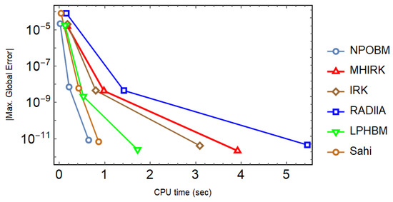
Figure 8.
Efficiency curves for the system in Problem 3 to observe the behavior of absolute maximum global errors versus the CPU time (sec) with a logarithmic scale on y-axis.
Problem 4
(Biomass Transfer [38]). Take, for example, a forest in Europe that only has one or two different kinds of trees. We begin by selecting some of the oldest trees, those that are forecast to pass away during the next several years, and then we trace the progression of live trees into dead ones. The dead trees will gradually rot and collapse due to the various biological and seasonal occurrences. In the end, the trees that have fallen form humus. Define the variables x, y, z, and t by the following:
- equals the biomass that has decomposed into humus;
- represents the biomass of dead trees;
- represents the biomass of live trees;
- equals the amount of time in decades (one decade equals ten years).
The differential equations for the above scenario are given below:
with initial condition , and . The exact solution is as follows:
Model (38) is simulated with different techniques, and the results are tabulated. Both constant and adaptive stepsize approaches are used. It can be seen in Table 13, Table 14 and Table 15 that the proposed technique (14) not only yields the minimum errors, but it also goes with the highest scd factor, thereby proving the much better performance of (14) in comparison to other well-known block techniques. In addition, the superiority of the proposed technique is maintained, even when the adaptive stepsize approach is utilized with varying values of the tolerance as shown in Table 16. It is also worth noting that method MHIRK could not produce promising results even utilizing 88 steps, whereas, in comparison, NPOBM outperforms. Finally, the efficiency curves produced with each technique under consideration speak volumes in favor of (14) since they take the shortest time to yield the smallest maximum absolute global error as shown in Figure 9.
Table 13.
Numerical results for Problem 4 with NS = where .
Table 14.
Numerical results for Problem 4 with NS = where .
Table 15.
Numerical results for Problem 4 with NS = , where .
Table 16.
Numerical results for Problem 4 with adaptive step-size approach while .
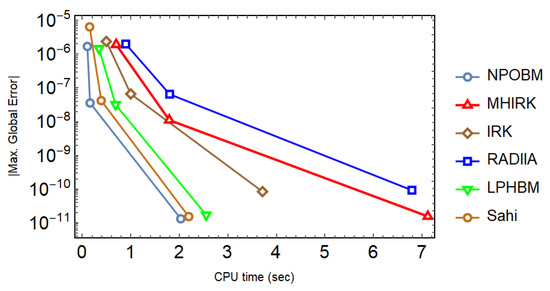
Figure 9.
Efficiency curves for the system in Problem 4 to observe the behavior of absolute maximum global errors versus the CPU time (sec) with a logarithmic scale on y-axis.
Problem 5.
We consider the following two-dimensional nonlinear system taken from Ref. [39]:
while the exact solution is with
Model (39) mentioned in Problem 5 is simulated with different techniques, and the results are tabulated. It can be seen in Table 17, Table 18 and Table 19 that the proposed technique (14) not only yields the minimum errors, but it also goes with the highest scd factor, thereby proving the much better performance of (14) in comparison to other well-known block techniques. It is also worth noting that method IRK failed to produce promising results even utilizing steps, whereas, in comparison, NPOBM outperforms.
Table 17.
Numerical results for Problem 5 with NS = where .
Table 18.
Numerical results for Problem 5 with NS = where .
Table 19.
Numerical results for Problem 5 with NS = where .
6. Concluding Remarks and Future Directions
By combining interpolation and collocation methods, a novel one-step optimized block method was devised, with a calculated order of convergence of at least five. The method’s theoretical analysis in this work shows that it is consistent, zero-stable, linear stable, aligned with the theory of order stars, and convergent; these properties allow it to successfully numerically solve a wide range of models that are stiff and nonlinear but appear in the applied and health sciences. Further, the method’s two off-grid spots are optimized based on the local truncation errors derived from a Taylor series. The suggested block method outperforms other similar methods from the literature, as demonstrated by numerical experiments selected from a variety of disciplines. When compared to others, the proposed method performs admirably, especially when it comes to the adaptive step-size strategy. With this in mind, the initial value problems of ordinary differential equations are a good candidate for the optimized block method suggested here. The order of convergence of the current optimized block method will be improved in the future to make it either - or -stable.
Author Contributions
The authors confirm their contribution to the paper as follows: K.A.: Conceptualization, Formal Analysis, Funding acquisition, Writing—original draft; S.Q.: Writing—original draft, Investigation, Methodology, Software; A.S.: Formal analysis, Software, Validation, Visualization; M.A.: Supervision, Writing—review and editing. All authors reviewed the results and approved the final version of the manuscript.
Funding
This work was supported by the Deanship of Scientific Research, Vice Presidency for Graduate Studies and Scientific Research, King Faisal University, Saudi Arabia [Grant No. 2569].
Institutional Review Board Statement
Not applicable.
Informed Consent Statement
Not applicable.
Data Availability Statement
Not applicable.
Conflicts of Interest
The authors declare no conflict of interest. The funders had no role in the design of the study; in the collection, analyses, or interpretation of data; in the writing of the manuscript; or in the decision to publish the results.
References
- Henrici, P. Discrete Variable Methods in Ordinary Differential Equations; Wiley: New York, NY, USA, 1962; Volume 6, p. 407. [Google Scholar]
- Grimshaw, R. Nonlinear Ordinary Differential Equations: Applied Mathematics and Engineering Science Texts; CRC Press: Boca Raton, NY, USA, 1993; pp. 1–367. [Google Scholar]
- Weinstock, R. Calculus of Variations: With Applications to Physics and Engineering; Dover Publications, Inc.: New York, NY, USA, 1974; pp. 1–321. [Google Scholar]
- Weiglhofer, W.S.; Lindsay, K.A. Ordinary Differential Equations and Applications: Mathematical Methods for Applied Mathematicians, Physicists, Engineers and Bioscientists; Elsevier: Amsterdam, The Netherlands, 1999; pp. 1–156. [Google Scholar]
- Li, H.; Peng, R.; Wang, Z.A. On a diffusive SIS epidemic model with mass action mechanism and birth-death effect: Analysis, simulations and comparison with other mechanisms. SIAM J. Appl. Math. 2018, 78, 2129–2153. [Google Scholar] [CrossRef]
- Xie, X.; Xie, B.; Xiong, D.; Hou, M.; Zuo, J.; Wei, G.; Chevallier, J. New theoretical ISM-K2 Bayesian network model for evaluating vaccination effectiveness. J. Ambient. Intell. Humaniz. Comput. 2022, 1–17. [Google Scholar] [CrossRef]
- Lyu, W.; Wang, Z.A. Logistic damping effect in chemotaxis models with density-suppressed motility. Adv. Nonlinear Anal. 2022, 12, 336–355. [Google Scholar] [CrossRef]
- Butcher, J.C. The Numerical Analysis of Ordinary Differential Equations: Runge-Kutta and General Linear Methods; Wiley-Interscience: Hoboken, NJ, USA, 1987. [Google Scholar]
- Brugnano, L.; Iavernaro, F.; Trigiante, D. The lack of continuity and the role of infinite and infinitesimal in numerical methods for ODEs: The case of symplecticity. Appl. Math. Comput. 2012, 218, 8056–8063. [Google Scholar] [CrossRef]
- Finizio, N.; Ladas, G. Ordinary Differential Equations with Modern Applications; Wadsworth Pub. Co.: Belmont, CA, USA, 1988. [Google Scholar]
- Gregus, M. Third Order Linear Differential Equations; De Reidel Publishing Company: Tokyo, Japan, 1987; pp. 86–3198. [Google Scholar]
- Roberts, S.B. Multimethods for the Efficient Solution of Multiscale Differential Equations. Doctoral Dissertation, Virginia Tech, Blacksburg, VA, USA, 2021; pp. 1–196. [Google Scholar]
- Prothero, A.; Robinson, A. On the stability and accuracy of one-step methods for solving stiff systems of ordinary differential equations. Math. Comput. 1974, 28, 145–162. [Google Scholar] [CrossRef]
- Tam, H.W. One-stage parallel methods for the numerical solution of ordinary differential equations. SIAM J. Comput. 1992, 13, 1039–1061. [Google Scholar] [CrossRef]
- Jator, S.N.; Li, J. A self-starting linear multistep method for a direct solution of the general second order initial value problem. Int. J. Comput. Math. 2007, 86, 817–836. [Google Scholar] [CrossRef]
- Shokri, A. A new eight-order symmetric two-step multiderivative method for the numerical solution of second-order IVPs with oscillating solutions. Numer. Algorithm 2018, 77, 95–109. [Google Scholar] [CrossRef]
- Ramos, H.; Rufai, M.A. A two-step hybrid block method with fourth derivatives for solving third-order boundary value problems. Comput. Appl. Math. 2022, 404, 113419. [Google Scholar] [CrossRef]
- Sunday, J.; Shokri, A.; Marian, D. Variable step hybrid block method for the approximation of Kepler problem. Fractal Fract. 2022, 6, 343. [Google Scholar] [CrossRef]
- Singh, G.; Ramos, H. An optimized two-step hybrid block method formulated in variable stepsize mode for integrating y” = f(x, y, y’) numerically. Numer. Math. Theory Methods Appl. 2019, 12, 640–660. [Google Scholar]
- Rufai, M.A.; Ramos, H. Numerical solution of second-order singular problems arising in astrophysics by combining a pair of one-step hybrid block Nyström methods. Astrophys. Space Sci. 2020, 365, 1–13. [Google Scholar] [CrossRef]
- Areo, E.A.; Rufai, M.A. A new uniform fourth order one-third step continuous block method for direct solutions of y” = f(x, y, y’). Br. J. Math. Comput. Sci. 2016, 15, 1–12. [Google Scholar] [CrossRef] [PubMed]
- Qureshi, S.; Soomro, A.; Hincal, E.; Lee, J.R.; Park, C.; Osman, M.S. An efficient variable stepsize rational method for stiff, singular and singularly perturbed problems. Alex. Eng. J. 2022, 61, 10953–10963. [Google Scholar] [CrossRef]
- Ramos, H. Development of a new Runge-Kutta method and its economical implementation. Comput. Math. Methods 2019, 1, e1016. [Google Scholar] [CrossRef]
- Qureshi, S.; Ramos, H.; Soomro, A.; Hincal, E. Time-efficient reformulation of the Lobatto III family of order eight. J. Comput. Sci. 2022, 63, 101792. [Google Scholar] [CrossRef]
- Ramos, H.; Rufai, M.A. Third derivative modification of k-step block Falkner methods for the numerical solution of second order initial value problems. Appl. Math. Comput. 2018, 333, 231–245. [Google Scholar] [CrossRef]
- Ramos, H.; Vigo-Aguiar, J. A new algorithm appropriate for solving singular and singularly perturbed autonomous initial-value problems. Int. J. Comput. Math. 2008, 603–611. [Google Scholar] [CrossRef]
- Dahlquist, G.G. A special stability problem for linear multistep methods. Bit Numer. Math. 1963, 3, 27–43. [Google Scholar] [CrossRef]
- Wanner, G.; Hairer, E. Solving Ordinary Differential Equations II; Springer: Berlin/Heidelberg, Germany, 1996; p. 375. [Google Scholar]
- Qureshi, S.; Ramos, H. L-stable explicit nonlinear method with constant and variable step-size formulation for solving initial value problems. Int. J. Nonlinear Sci. Numer. 2018, 19, 741–751. [Google Scholar] [CrossRef]
- Akinfenwa, O.A.; Okunuga, S.A.; Akinnukawe, B.I.; Rufai, U.P.; Abdulganiy, R.I. Multi-derivative hybrid implicit Runge-Kutta method for solving stiff system of a first order differential equation. Far East J. Math. Sci. 2018, 106, 543–562. [Google Scholar]
- Butcher, J.C. Numerical Methods for Ordinary Differential Equations; John Wiley & Sons: Hoboken, NJ, USA, 2016. [Google Scholar]
- Sahi, R.K.; Jator, S.N.; Khan, N.A. A Simpson’s-type second derivative method for stiff systems. Int. J. Pure Appl. Math. 2012, 81, 619–633. [Google Scholar]
- Sunday, J.; Kolawole, F.M.; Ibijola, E.A.; Ogunrinde, R.B. Two-step Laguerre polynomial hybrid block method for stiff and oscillatory first-order ordinary differential equations. J. Math. Comput. Sci. 2015, 5, 658–668. [Google Scholar]
- Rufai, M.A.; Duromola, M.K.; Ganiyu, A.A. Derivation of one-sixth hybrid block method for solving general first order ordinary differential equations. IOSR-JM 2016, 12, 20–27. [Google Scholar]
- Jenny, K.; Käppeli, O.; Fiechter, A. Biosurfactants from Bacillus licheniformis: Structural analysis and characterization. Appl. Microbiol. Biotechnol. 1991, 36, 5–13. [Google Scholar] [CrossRef] [PubMed]
- Alvarez, C.M.; Litchfield, R.; Jackowski, D.; Griffin, S.; Kirkley, A. A prospective, double-blind, randomized clinical trial comparing subacromial injection of betamethasone and xylocaine to xylocaine alone in chronic rotator cuff tendinosis. Am. J. Sports Med. 2005, 33, 255–262. [Google Scholar] [CrossRef] [PubMed]
- Horgan, M.J. Differential Structuring of Reservoir Phytoplankton and Nutrient Dynamics by Nitrate and Ammonium. Doctoral Dissertation, Miami University, Oxford, OH, USA, 2005. [Google Scholar]
- May, R.; McLean, A.R. Theoretical Ecology: Principles and Applications; Oxford University Press on Demand: Oxford, UK, 2007. [Google Scholar]
- Ramos, H.; Singh, G. A note on variable step-size formulation of a Simpson’s-type second derivative block method for solving stiff systems. Appl. Math. Lett. 2017, 64, 101–107. [Google Scholar] [CrossRef]


Disclaimer/Publisher’s Note: The statements, opinions and data contained in all publications are solely those of the individual author(s) and contributor(s) and not of MDPI and/or the editor(s). MDPI and/or the editor(s) disclaim responsibility for any injury to people or property resulting from any ideas, methods, instructions or products referred to in the content. |
© 2023 by the authors. Licensee MDPI, Basel, Switzerland. This article is an open access article distributed under the terms and conditions of the Creative Commons Attribution (CC BY) license (https://creativecommons.org/licenses/by/4.0/).