Mathematical and Statistical Modelling for Assessing COVID-19 Superspreader Contagion: Analysis of Geographical Heterogeneous Impacts from Public Events

Abstract

During a pandemic, public discussion and decision-making may be required in face of limited evidence. Data-grounded analysis can support decision-makers in such contexts, contributing to inform public policies. We present an empirical analysis method based on regression modelling and hypotheses testing to assess events for the possibility of occurrence of superspreading contagion with geographically heterogeneous impacts. We demonstrate the method by evaluating the case of the May 1st, 2020 Demonstration in Lisbon, Portugal, on regional growth patterns of COVID-19 cases. The methodology enabled concluding that the counties associated with the change in the growth pattern were those where likely means of travel to the demonstration were chartered buses or private cars, rather than subway or trains. Consequently, superspreading was likely due to travelling to/from the event, not from participating in it. The method is straightforward, prescribing systematic steps. Its application to events subject to media controversy enables extracting well founded conclusions, contributing to informed public discussion and decision-making, within a short time frame of the event occurring.

1. Introduction

On December 2019, a new Coronavirus Disease 2019 (COVID-19) characterized by high levels of transmission, was reported in the city of Wuhan in the province of Hubei in China. Spreading quickly, its serious damage was felt all over the world on human health and indirectly on many other areas. Decision-making on public policies was required with limited or conflicting information on topics such as masking, distancing, and outdoor vs. indoor gatherings, among others.

Mathematical and statistical based approaches have been widely used to predict the spread of COVID-19 in many countries and regions, as we can see in review papers [1,2,3]. While COVID-19 remains a serious disease worldwide, the combination of factors, such as vaccination and natural immunity, among others, has now lessened overall public concerns and policies. However, epidemics and pandemics are regular events that humanity faces, where effective decision-making on public policies must be made with limited prior information.

We intend to contribute to inform public discussion and decision-making in such contexts, by enabling data-driven conclusions about possible effects of events on regional contagion patterns. With this aim, this work provides a statistical modelling method, exemplified with the case of a large-scale public event held in Lisbon, Portugal, at an early stage in the pandemic in 2020: the May 1st demonstration.

To check if an event had or not impact on its region vs. the rest of the country, and if any effect would exhibit significant differences among counties in the region, our empirical analysis method is based on regression modelling and hypotheses testing, on data matching two time frames: a period where possible event contagion has not yet been reported, and a period where any such contagion would expectably have been reported. We defined these periods using the virus incubation period and the reporting delay in notification of positive cases. We then analyzed county-level cumulative new daily cases, and defined both linear and exponential models for each, with the dependent variable being the cumulative number of COVID-19 cases in the counties of Lisbon metropolitan area. The independent variable was the number t of days since 15 April.

By applying the proposed method to this event, we concluded that the event likely caused a change in the growth pattern of new COVID-19 cases in the Lisbon region, accelerating the rate of change compared to what it was before the event was held. This did not happen in the rest of the country, which was stabilizing growth rate and kept that trend in the period where potential event impact would have been reported. It was also possible to conclude that counties with greatest contributions to change in the growth pattern of the Lisbon region were those from which the likely means of transportation for the event were not subway or trains, but chartered buses or private vehicles, and with the longest car travel time.

The main contribution of this work is the innovative method, designed for analyzing events in a pandemic/epidemic context, where public decision-making is required with limited available information on potential impact factors. This analysis method enables identification of the geographical differences of the impact of events on contagion dynamics and exploration of mechanisms that may anticipate its existence. It can be replicated to analyze impact hypotheses of other events and explore other factors that can explain those impacts, contributing to data-grounded decision-making on public policies and hopefully to better health and save lives.

2. Background

2.1. COVID-19

COVID-19 positive case numbers notified by health authorities in Portugal are those “with laboratory confirmation of SARS-CoV-2, regardless of symptoms and signs” [4]. Early in the pandemic in Portugal (from March 2020 onwards), tests on individuals with symptoms were almost only performed in hospital emergency units [5] or in contact screening procedures [6]. Thus, for contagion in events or other social activities (travel, meals, socializing, etc.), emergence of new cases in national public statistics must consider the time until symptoms arise: the incubation period. Lauer et al. [7] estimated a median incubation period of 5.1 days [95% Confidence Interval (CI): 4.5–5.8 days] and a mean of 5.5 days, with less than 2.5% of the infected showing symptoms at 2.2 days after contagion, and 97.5% of the cases showed symptoms at 11.5 days after the infection.

Further, after symptoms emerge, it is necessary that the person is tested, the test yields an outcome, that authorities are notified, and that official statistics are published. This is known as “reporting delay”. Our rationale for Portugal was that, for a person with symptoms to seek healthcare structures and take a test, it would take one day; the result of the test should be available on that same day or up to two days later, since, at the time, Portugal depended exclusively on reverse transcription-polymerase chain reaction (RT-PCR) tests, having no rapid diagnostic tests available [8]. Additionally, once the diagnosis is made, it is expected that the individual is included in the national statistics’ report the following day. Therefore, from onset of symptoms, a reporting delay of four days is expected. This rationale was supported by the Portuguese Directorate-General of Health (DGH), which, on 19 October, in a regular press conference on the COVID-19 pandemic in Portugal, mentioned a three-day period between the onset of symptoms and the diagnosis, which results in a mean period of four days from onset of symptoms until impact on public reports [9].

This reasoning supports the definition of two periods of time whose COVID-19 spread dynamics will be compared: one prior to the influence of potential infections during the event and another where it is expected that any infection that occurred during the event has already been reported.

2.2. Growth Models

Over time, since the COVID-19 pandemic was declared, many mathematical premise-based-only models have been adopted. However, there are many non-quantifiable factors, such as the occurrence of large events, changes in transportation policies, public health strategies, and sociodemographic characteristics of the population that may substantially affect predictions on the epidemiologic curve evolution and whose influence on the disease dynamics has been researched [10,11,12].

Common modulation strategy of cumulative number of COVID-19 cases to predict pandemic evolution relies on S-shaped (sigmoid) growth curves [13], to see graphically the predictable curve behavior within subsequent days. These curves are generally based on well known cumulative distribution functions, such as Gompertz distribution, logistic, log-normal, and Gumbel distributions, which are particular cases of the sigmoid curve. Additionally, as a particular case, Richards traditional growth curve [14] assumes that the cumulative number of disease cases in time t is given by the expression (1):

$$C\left(t\right)=\frac{A}{{[1+mexp(-k(x-i))]}^{\frac{1}{m}}}.$$

(1)

This parametrization of Richards curve presents an adequate structure for infectious disease modelling [15,16]. Wang et al. [17] provide biological interpretations to all of the parameters in this model and introduce a constraint to address overfitting problem observed in some existing studies. In the above Formula (1), A is the number of cumulative cases at the end of the epidemic period under study, k is the growth index per capita of the number of cumulative cases, m is the shape parameter (exponent used to capture the symmetry deviation in the S-shaped dynamics of the simple logistic model), and i is the lag phase of the trajectory. It has been used in modelling for real-time prediction in infectious outbreaks [15,17,18,19,20,21,22,23].

When epidemic evolution shows two or more successive sigmoids, a double Richards model becomes adequate, defined by combining two regular Richards models (2). The package FlexParamCurve [24] implements this model, providing a wide range of versions that depend on parameters across the dataset. Specifying the parameters m = 1, m = 0 or m = −0.3 the Logistic, Gompertz, and von Bertalanffy curves are obtained.

$$\begin{array}{c}\hfill C\left(t\right)=\frac{A}{{[1+mexp(-k(x-i))]}^{\frac{1}{m}}}+\frac{A^{\prime }}{{[1+m^{\prime }exp(-k^{\prime }(x-i^{\prime }))]}^{\frac{1}{m^{\prime }}}}.\end{array}$$

(2)

The previous models reflect dynamics whose complexity requires some time to be noticeable. Over short periods of time, the dynamics of infection practically do not change, and public awareness and containment actions change very little, hence the contagion dynamics remain stable. Thus, the effort of analysis over short time periods with the previous models is not justified because the underlying dynamics can be captured by simpler models, due to the stability of contagion dynamics for those periods. This option for simpler models meets the principle of parsimony in the selection of models [25], which establishes that, between two competing models in terms of goodness-of-fit, the simpler one must be selected, that is, the one with less parameters.

Thus, for short time periods, under analysis in this work, we chose to fit linear and exponential models (models (3) and (4)) to the data, using R package stats and lm () function. The independent variable X is the number of days since 15 April 2022, and the dependent variable Y is the cumulative number of COVID-19 cases.

Let X denote the random independent variable and Y denote the response variable. We then define:

$$\mathrm{Linear}\mathrm{model}:Y={\beta }_0+{\beta }_{1}X+\epsilon ,\mathrm{with}\epsilon \sim N(0,{\sigma }^2)\mathrm{and}iid.$$

(3)

$$\mathrm{Exponential}\mathrm{model}:ln\left(Y\right)={\beta }_0+{\beta }_{1}X+\epsilon ,\mathrm{with}\epsilon \sim N(0,{\sigma }^2)\mathrm{and}iid.$$

(4)

The coefficients are estimated by the ordinary least squares method from a random sample $\left(X_t,Y_t\right),t=1,2,\cdots ,n$.

To assess the accuracy of the models and the goodness-of-fit, one can use the adjusted coefficient of determination (adjusted $R^2$) and the root mean square error (RMSE), among others. To assess the overall quality of the models one can use the F-statistic. If the numerical value of RMSE is small, the discrepancy between oberved data and predict values by the model is small, and the model accuracy increases. As the value of $R^2$ increases (approaches the unity), the model has high accuracy [2].

2.3. General Methodological Approach

Our empirical analysis method checks whether an event had an impact or not on its region vs. the rest of the country. It also checks for significant differences among counties in the region, for any such effect. It employs regression modelling and hypotheses testing, based on data along two time frames: one is a period where possible event contagion has not yet been reported, and another is a period where any such contagion would expectably have been reported. These periods are based on the virus incubation period and reporting delay in notification of positive cases, and analyzed for county-level cumulative new daily cases, defining linear and exponential models for each, relating the cumulative number of COVID-19 cases in the counties of the Lisbon metropolitan area (dependent variable) and the number t of days since 15 April (independent variable).

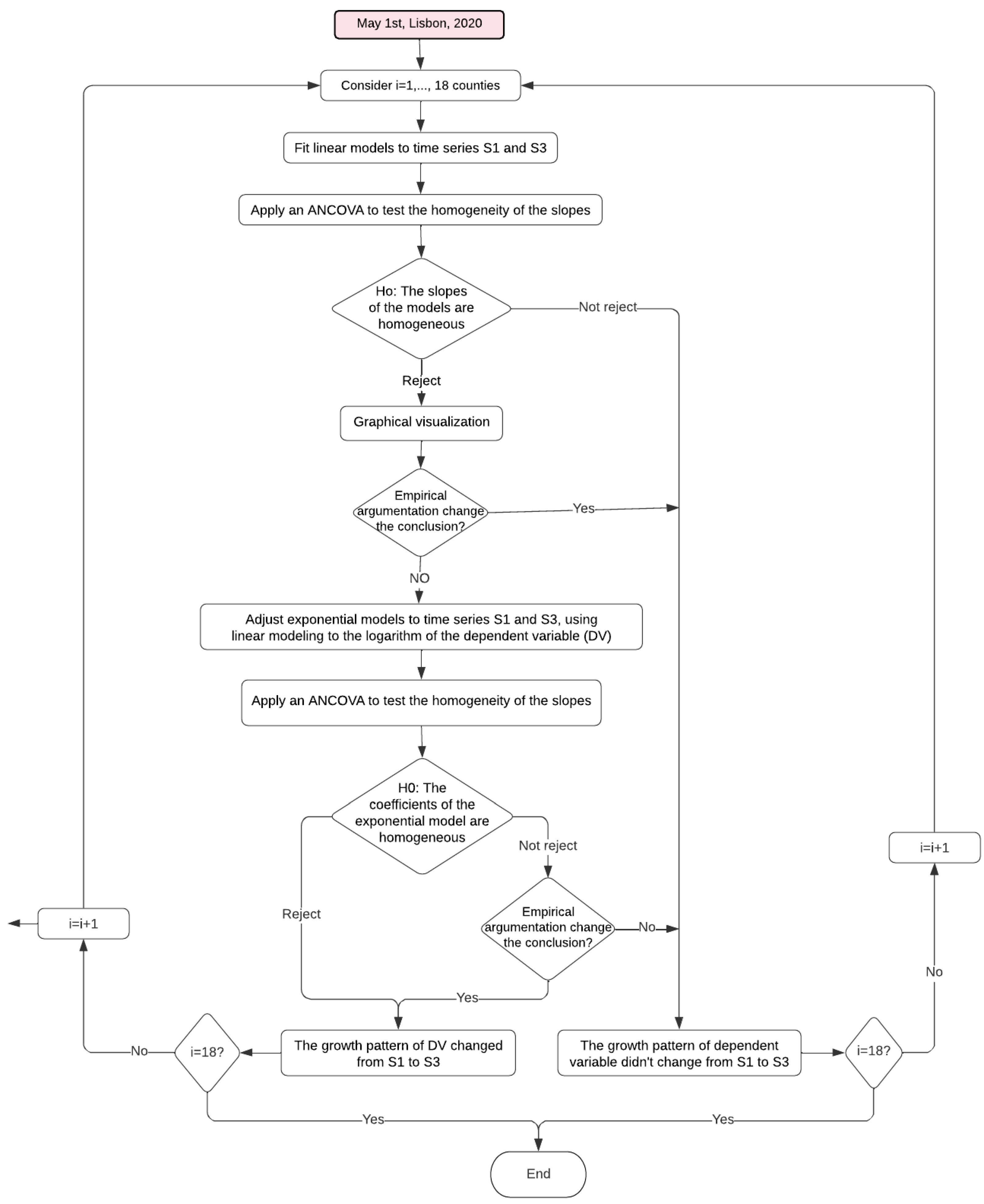
Systematically, we use one-way analysis of covariance (ANCOVA) with interaction for testing coefficient homogeneity of the linear models in each period [26], and we employ graphical visualization to verify the nature of differences, when the homogeneity of rate of change hypothesis is rejected. Counties are grouped by: those where the homogeneity hypothesis is rejected; those where the hypothesis of no changes in the growth pattern after the event is not rejected; and those where the growth of COVID-19 cases accelerates post-event.

Any counties where the homogeneity of rate of change hypothesis is not rejected for linear models that we fitted to both periods, i.e., for which the maintenance of growth pattern post-event hypothesis is not rejected, and also any counties where this hypothesis is rejected but graphical visualization or coefficient comparison concludes there was no case growth acceleration between the periods, are all included in the county group with no growth pattern change of the dependent variable (the cumulative number of COVID-19 cases in the counties of the Lisbon metropolitan area). For the others, we test homogeneity of exponential model coefficients. Subsequently:

1.

we place counties of rejected homogeneity of exponential model coefficients in the group exhibiting case growth acceleration between periods;

2.

counties with case growth rate acceleration between periods (homogeneity of slopes in linear models was reject), but non-rejected coefficient homogeneity for exponential models fitted to both periods, have the first period enlarged until the earliest available day of county-level data to assess the best fit (linear/exponential) for each period.

3. The Case under Analysis

3.1. The 1st of May 2020 Demonstration in Lisbon

In 2020, the May 1st Demonstration (Labour Day) occurred during the state of emergency declared to contain the pandemic, between 19 March and 2 May [27]. State of emergency rules precluded travel between counties and gatherings, except for political and labour unions activities, which allowed this demonstration.

According to the organizing body, CGTP-IN (the largest trade union federation in Portugal, Portuguese-language acronym), participants came from the metropolitan area and part of them came in individual transportation or in buses whose occupancy did not exceed one third of maximum capacity” [28]. According to media reports there were about one thousand participants, keeping social distancing and sanitary rules, including the use of masks [29].

3.2. The Lisbon Metropolitan Area

The Lisbon Metropolitan Area (AML, Portuguese-language acronym) is the group of counties from where most of the May 1st 2020 demonstrators travelled, by individual cars or rented buses, according to the CGTP-IN press release cited above. It is a legal association of counties, composed by: Alcochete, Almada, Amadora, Barreiro, Cascais, Lisbon, Loures, Mafra, Moita, Montijo, Odivelas, Oeiras, Palmela, Seixal, Sesimbra, Setúbal, Sintra, and Vila Franca de Xira [30]. Lisbon, the country capital and main city in the region, is the centripetal location of transportation networks. The location of the May 1st demonstration is quite central within Lisbon itself.

By considering the available public transportation options from the counties to the demonstration site, the estimated travel time on a public holiday, convenience of transportation, and public statements mentioned above on combined individual and bus travel for the demonstration, we grouped counties by estimated form of transport.

Group 1: Demonstrators from counties with good public transport connections of trains and subways that can be reached in under an hour were presumed to have taken those forms of transport. These include transportation in the following areas: Lisbon, Odivelas, Amadora, Sintra, Oeiras, Almada, Cascais, Vila Franca de Xira.

Group 2: Demonstrators without such transport connections were thought to have travelled in private vehicles or hired buses. Loures, Seixal, Barreiro, Mafra, Moita, Setúbal, Montijo, Palmela, Sesimbra, Alcochete.

3.3. Data

Data on the cumulative number of COVID-19 cases in Portuguese counties, including those of AML, come from the daily situation reports issued from 24 March to 6 June 2020 by DGH. Data were collected daily by the authors, directly from the official reports and from the online repository of the “Data Science for Social Good Portugal” community, which extracts these data daily and makes them publicly available at https://github.com/dssg-pt/covid19pt-data (accessed on 28 December 2022).

4. Methodology

4.1. Rationale for Defining Given Key Issues

The starting hypothesis admits that the possibility of an event having a superspreading effect is not homogeneous in the surrounding region. This stems from the different contexts of contagion risk during a potentially superspreading event: (a) contagion during the event itself, from which one would not expect differentiated effects on participants’ home counties; and (b) in the course of travel to or from the event, where different conditions of contagion could lead to different effects in the counties of origin of the participants.

Thus, two assumptions are raised, one about the effect of the event on the region and the other on whether this was the same for each county in the region:

Q1: The event had no effect on the contagion rate in the region of origin of the participants, compared to the rest of the country.

Q2: The effect of the event on the region of origin of the participants had no geographical differences in the rate of contagion.

4.2. Methodological Procedure for Data Analysis

For assumption Q1, we analyze the contagion pattern in the region vs. the rest of the country, before and after the time window of potential development of event contagion effects, to verify if they are identical or not. If they are, one will not reckon that there was an event impact, assuming participation is predominantly by inhabitants of the area. In the current case, this is shown in Section 5.3. For Q2, we analyzed contagion patterns before and after the same time window for each county in the region. This is shown for the current case in Section 5.4.

These preliminary analyses determine whether the assumptions are moot or whether further analysis is required to answer them. If so, to assess the assumption, an empirical methodology was devised based on regression modelling, hypothesis tests, and graphical visualization. We define three periods: Period S1, when any contagion cases at the event are not yet being reported; Intermediate Period S2, when they are undergoing reporting; and the Final Period S3, when almost any such cases have been reported. This is detailed below in Section 5.2. The Intermediate Period S2 is not considered in the analysis, which compares periods S1 and S3, i.e., “without potential effects from the event” and “with total potential effects from the event”, respectively. Then, we compare the target periods under analysis by modelling their contagion behavior and comparing the behavior of their respective models. The contagion behaviour in periods S1–S3 may follow linear or exponential models, depending on the degree of transmissibility. Typically, there is no inflection point in the growth curves because that case would be trivial. Therefore, linear and exponential models were fitted for each period: to the data from the region, to the data of the rest of the country, and to the data from each county. For the current case, our models’ fit was assessed at a statistical significance level of 5%.

The procedure to analyze the contagion dynamics in the counties (Q2) has four stages. First, contagion behavior between periods S1 and S3 is compared using linear models and ANCOVA tests to test their slope homogeneity to determine in which counties the hypothesis of no change in the post-event growth pattern of COVID-19 cases is not rejected, at 5% significance level. These counties are assigned to the category of locations where there were probably no effects of the event.

Second, the slopes of models in which homogeneity is rejected are visually compared to detect counties where the growth rate decreased or where case growth was an artifact, e.g., due to a sudden increase occurring in the Intermediate Period S2, after which the slope returns (in the model fit to S3) to values similar to those of the model fitted to S1. These counties are also assigned to the category of places where there were probably no effects from the event.

Third, for counties with an increase in linear growth rate, we analyze the possibility that it simply reflects growth from a previous ongoing exponential contagion, not the effects of the event under analysis. For this, we test homogeneity of coefficients of the exponential models. The counties where, even with exponential models, the hypothesis of homogeneity is rejected, are assigned to the category of counties where there may have been effects of the event due to the acceleration in case growth.

Fourth, we analyze cases where one rejects the hypothesis of no change in linear growth pattern at 5% significance level, but not the hypothesis of homogeneity of coefficients of exponential models, at the same significance level. We scrutinize cases when from S1 to S3 there were changes in the type of model with the best fit. For instance, in our current case, an anomalous situation was found (Loures county), in which an exponential model in period S1 gave way to a linear model in Period S3 (with a very steep slope)—a behaviour contrary to contagion dynamics. In Section 6, we provide details on the analysis and resolution of this anomaly.

The flowchart (Figure 1) illustrates the methodology to assess assumptions Q1 and Q2.

5. Applying the Methodology to the Lisbon May 1st Demonstration Case

5.1. Preliminary Analysis

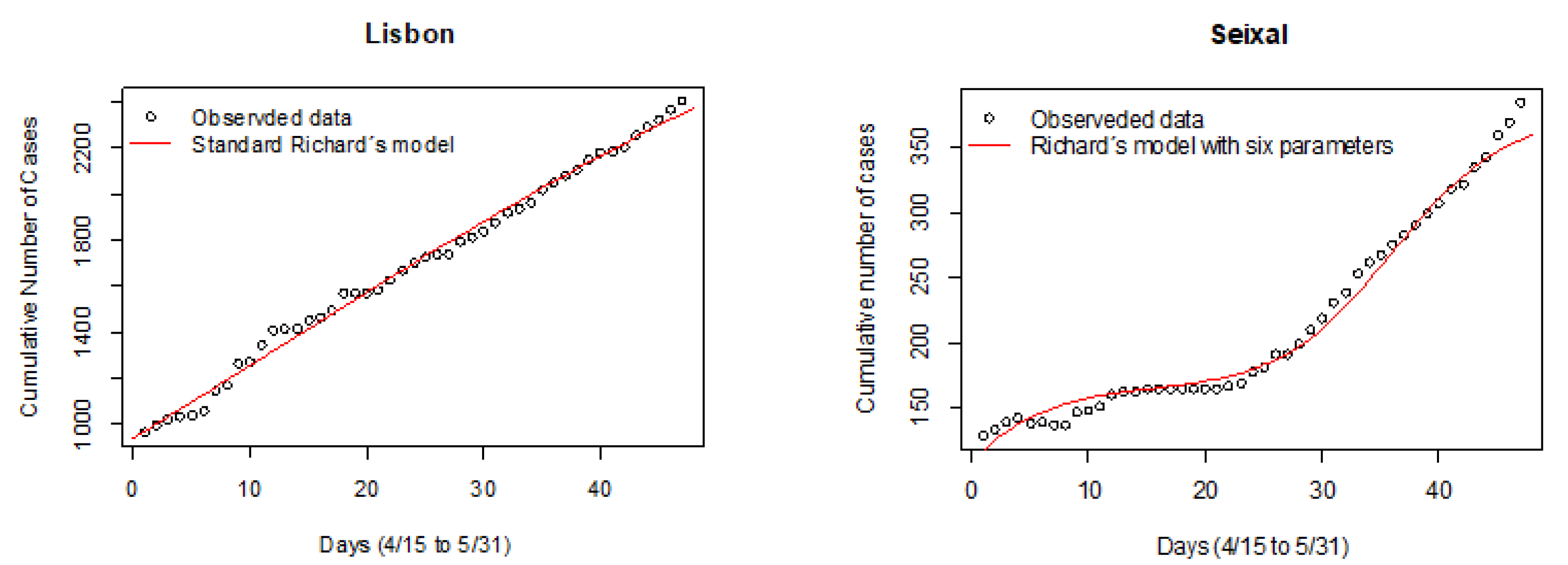
We employed graphical visualization to answer Q1 and Q2, using FlexParamCurve [24] to fit a double Richards model to cumulative cases of the AML region, of the rest of mainland Portugal, and of AML counties, between 15 April–31 May. For Q1, acceleration in contagion rate in the AML region was detected after the window of potential development of contagion effects, contrary to the rest of the country, whose contagion rate slowed down. For Q2 (individual counties analysis), we saw behaviors indicating potential influence of the May 1st Demonstration on the evolution of cumulative numbers of cases in some counties, and not in others (e.g., in Figure 2). Thus, the next analysis stages are needed.

5.2. Time Series Segmentation

Applying the method to the current case, the cases’ time series S from 15 April–6 June 2020 was divided into three segments, matching Periods S1, S2, and S3. This required identifying when potential contagion from the event started and ended being reported. From the literature (Section 2.1) until 2.2 days from contagion, less than 2.5% infected show symptoms [7], and then there was a four-day reporting delay. An extremely small number of cases of infection on 1 May will have been reported until the day before those two periods expire (6 May). So, the S1 refers to 15 April–6 May. Since 97.5% of the infected show symptoms within 11.5 days, plus the four-day reporting delay, the intermediate period with any event contagion reporting underway runs from 7–15 May: Period S2, the second segment. The final Period S3 is the rest of the series, 16 May–6 June, when practically all contagion cases from 1 May and onwards have already been reported.

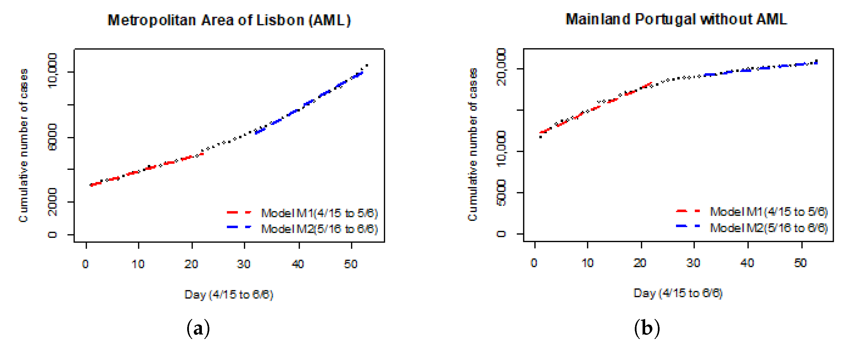
5.3. Rate of Change of Cumulative Cases in the AML Region and the Rest of the Country

Per the method, we compare the cumulative cases growth patterns between the AML region and the rest of mainland Portugal (Q1), defining the following hypotheses:

H0. 

There was no difference in case growth pattern in AML, vs. Rest of mainland Portugal.

H1. 

There was a difference in case growth pattern in AML, vs. Rest of mainland Portugal.

The comparison uses time series segments S1 & S3. To estimate the rate of change of cumulative cases, a linear model (5) was fit to each period (to S1: model M1, 15 April–6 May; to S3: model M2, 16 May–6 June), as shown in Figure 3.

$$\begin{array}{c}\hfill M1,M2:NCases={\beta }_0+{\beta }_{1}t+\epsilon ,\mathrm{with}\epsilon \sim N(0,{\sigma }^2)\mathrm{and}iid.\\ \hfill t\mathrm{is}\mathrm{the}\mathrm{number}\mathrm{of}\mathrm{days}\sin \mathrm{ce}15\mathrm{April}.\end{array}$$

(5)

To test the homogeneity of slopes of the models M1 and Me and, consequently, evaluate the statistical significance of the difference in cumulative cases growth rates, we fit a linear model with interaction between the variable t and the variable Dummy (which takes the value 0 for the S1 period and the value 1 for the S3 period) to the data set $S_1\bigcup S_3$ (model M3 (6)). Then, we implement an ANCOVA test to evaluate the statistical significance of the interaction term between the variable t and the two temporal periods under analysis, S1 and S3 [26]. If the interaction term is significant, it indicates that the slope of the line fit to the S3 data is significantly different from the slope of the line fit to the S1 data.

$$\begin{array}{c}\hfill M3:NCases={\beta }_0+{\beta }_{1}t+{\beta }_{3}Dummy+\gamma Dummy\times t+\epsilon \\ \hfill \epsilon \mathrm{is}\mathrm{iid}\mathrm{and}\epsilon \sim N(0,{\sigma }^2).\end{array}$$

(6)

ANCOVA tests applied to M3, with R package car [31], tested the hypotheses:

$$H_{0ANC}:\gamma =0\mathit{versus}{H}_{1ANC}:\gamma \ne 0.$$

(7)

Between AML and the rest of mainland Portugal (i.e., without AML counties), the difference in linear model coefficients proved statistically significant, at 5% level (p-value < 2.2 $\times {10}^{-16}$). The hypothesis of slope homogeneity, $H_{0ANC}$ (7), is rejected. In other words, the contagion rate, both in AML and the rest of the country, changed from S1 to S3, from a linear models perspective. However, in the rest of mainland Portugal (without AML counties) from the S1 period to S3, the coefficients showed a reduction (slowing down the case growth rate), while in AML, the coefficients increased (the case growth rate increased), thus the difference in growth pattern is clear in both cases (as shown in

Table 1. Linear models coefficients fit to data from AML and the rest of mainland Portugal.

	Linear Models
	M1	M2
	${\mathbf{\beta }}_{\mathbf{1}}$
Mainland Portugal (without counties from AML)	287.356	74.719
AML	93.583	188.584

). Consequently, the $H_0$ hypothesis is rejected.

5.4. Analysis of the Rate of Change of Cumulative Cases, by County

5.4.1. Formalizing the Hypotheses

Since preliminary analysis indicated potential influence of the event on the evolution of cumulative cases in some counties while not in others, for Q2 we formulated the following hypotheses for each county in the AML region (i = 1, 2, …, 18):

H_0i. 

There was no change in growth rate of cumulative number of cases in the county i.

H_1i. 

There was change in growth rate of cumulative number of cases in the county i.

5.4.2. Models, Hypotheses Tests, and Some Results

Per the first stage of the method, we estimated the rate of change in cumulative cases in each county, for periods S1 & S3, by fitting linear models (8) for each county i (i = 1, 2, …, 18). For S1, models $M{1}_i$: 15 April–6 May and for S3, models $M{2}_i$: 16 May–6 June.

$$\begin{array}{c}\hfill M{1}_i,M{2}_i:NCase{s}_i={\beta }_{0i}+{\beta }_{1i}t+{\epsilon }_i,\mathrm{with}{\epsilon }_i\sim N(0,{\sigma }^2)\mathrm{and}iid.\end{array}$$

(8)

To test slope homogeneity of models $M{1}_i$ and $M{2}_i$, for counties i (i = 1, 2, ..., 18) and, consequently, evaluate the statistical significance of the change rate of the cumulative number of cases between the two periods, a linear model with interaction (Equation (9)) between the variable “Number of days from 15 April” (t) and the Dummy variable defined previously, was fit to the data set $S_1\cup S_3$ (model 6) (

Table 2. Results from goodness-of-fit tests of M1 and M2 linear models (8) and their slope homogeneity, for each county.

	M1(4/15 to 5/6)		M2 (5/16 to 6/6)		M3 (Linear Model with Interaction: Group/Time)
						ANCOVA
County	Adjusted R Square	p-Value	Adjusted R Square	p-Value	p-Value	p-Value (Slope Comparison)
Alcochete	0.8074	8.34 $\times {10}^{-09}$	0.392	0.001	<2.2 $\times {10}^{-16}$	0.0003 ***
Almada	0.8956	1.742 $\times {10}^{-11}$	0.9912	2.2 $\times {10}^{-16}$	<2.2 $\times {10}^{-16}$	0.0923
Amadora	0.948	1.604 $\times {10}^{-14}$	0.9807	<2.2 $\times {10}^{-16}$	<2.2 $\times {10}^{-16}$	2 $\times {10}^{-16}$ ***
Barreiro	0.8438	1.005 $\times {10}^{-09}$	0.9696	<2.2 $\times {10}^{-16}$	<2.2 $\times {10}^{-16}$	<2.2 $\times {10}^{-16}$ ***
Cascais	0.9711	2.686 $\times {10}^{-16}$	0.9866	<2.2 $\times {10}^{-16}$	<2.2 $\times {10}^{-16}$	1.93 $\times {10}^{-10}$ ***
Lisbon	0.9711	<2.2 $\times {10}^{-16}$	0.9971	<2.2 $\times {10}^{-16}$	<2.2 $\times {10}^{-16}$	0.104
Loures	0.962	6.897 $\times {10}^{-16}$	0.9953	<2.2 $\times {10}^{-16}$	<2.2 $\times {10}^{-16}$	<2 $\times {10}^{-16}$ ***
Mafra	0.7822	2.881 $\times {10}^{-08}$	0.9685	<2.2 $\times {10}^{-16}$	<2.2 $\times {10}^{-16}$	2.671e $\times {10}^{-13}$ ***
Moita	0.8021	1.095 $\times {10}^{-08}$	0.9912	<2.2 $\times {10}^{-16}$	<2.2 $\times {10}^{-16}$	<2 $\times {10}^{-16}$ ***
Montijo	0.7301	2.535 $\times {10}^{-07}$	0.8869	3.915 $\times {10}^{-11}$	<2.2 $\times {10}^{-16}$	0.0004615 ***
Odivelas	0.9906	<2.2 $\times {10}^{-16}$	0.9944	<2.2 $\times {10}^{-16}$	<2.2 $\times {10}^{-16}$	<2 $\times {10}^{-16}$ ***
Oeiras	0.764	6.501 $\times {10}^{-08}$	0.9839	<2.2 $\times {10}^{-16}$	<2.2 $\times {10}^{-16}$	6.429 $\times {10}^{-16}$ ***
Palmela	−0.04059	0.6751	0.9124	2.984 $\times {10}^{-12}$	<2.2 $\times {10}^{-16}$	9.029 $\times {10}^{-12}$ ***
Seixal	0.8745	1.113 $\times {10}^{-10}$	0.9929	<2.2 $\times {10}^{-16}$	<2.2 $\times {10}^{-16}$	<2 $\times {10}^{-16}$ ***
Sesimbra	0.2056	0.01964	0.9665	<2.2 $\times {10}^{-16}$	<2.2 $\times {10}^{-16}$	<2 $\times {10}^{-16}$ ***
Setúbal	−0.02837	0.5112	0.9573	1.105 $\times {10}^{-14}$	<2.2 $\times {10}^{-16}$	<2 $\times {10}^{-16}$ ***
Sintra	0.9731	<2.2 $\times {10}^{-16}$	0.9285	3.926 $\times {10}^{-13}$	<2.2 $\times {10}^{-16}$	<2 $\times {10}^{-16}$ ***
Vila Franca de Xira	0.9542	4.448 $\times {10}^{-15}$	0.981	<2.2 $\times {10}^{-16}$	<2.2 $\times {10}^{-16}$	0.2032

(1) ″***″ The p-value is approximately zero. (2) Red color identifies the counties in which the goodness-of-fit test is not significant at a significance level of 5%.

).

$$\begin{array}{c}\hfill M{3}_i:NCase{s}_i={\beta }_{0i}+{\beta }_{1i}t+{\beta }_{3i}Dumm{y}_i+{\gamma }_{i}Dumm{y}_i\times t+{\epsilon }_i\\ \hfill \epsilon \mathrm{is}\mathrm{iid}\mathrm{and}\epsilon \sim N(0,{\sigma }^2),i=1,2,\cdots ,18.\end{array}$$

(9)

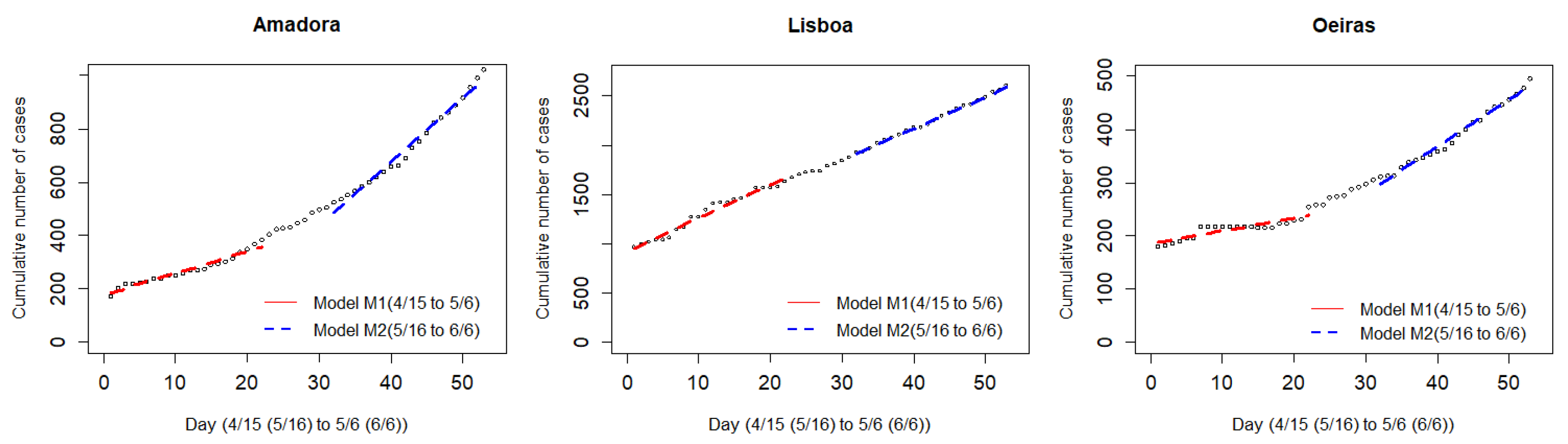
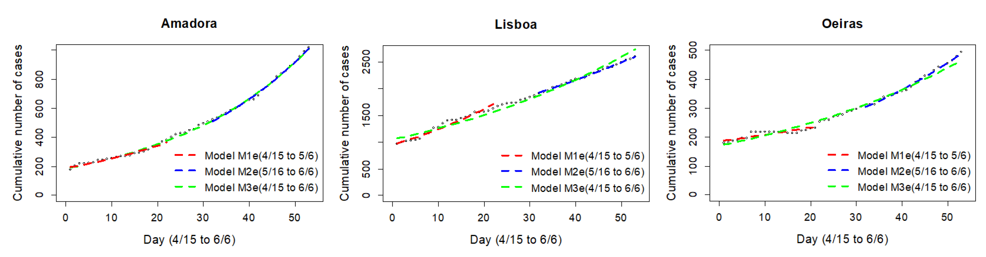
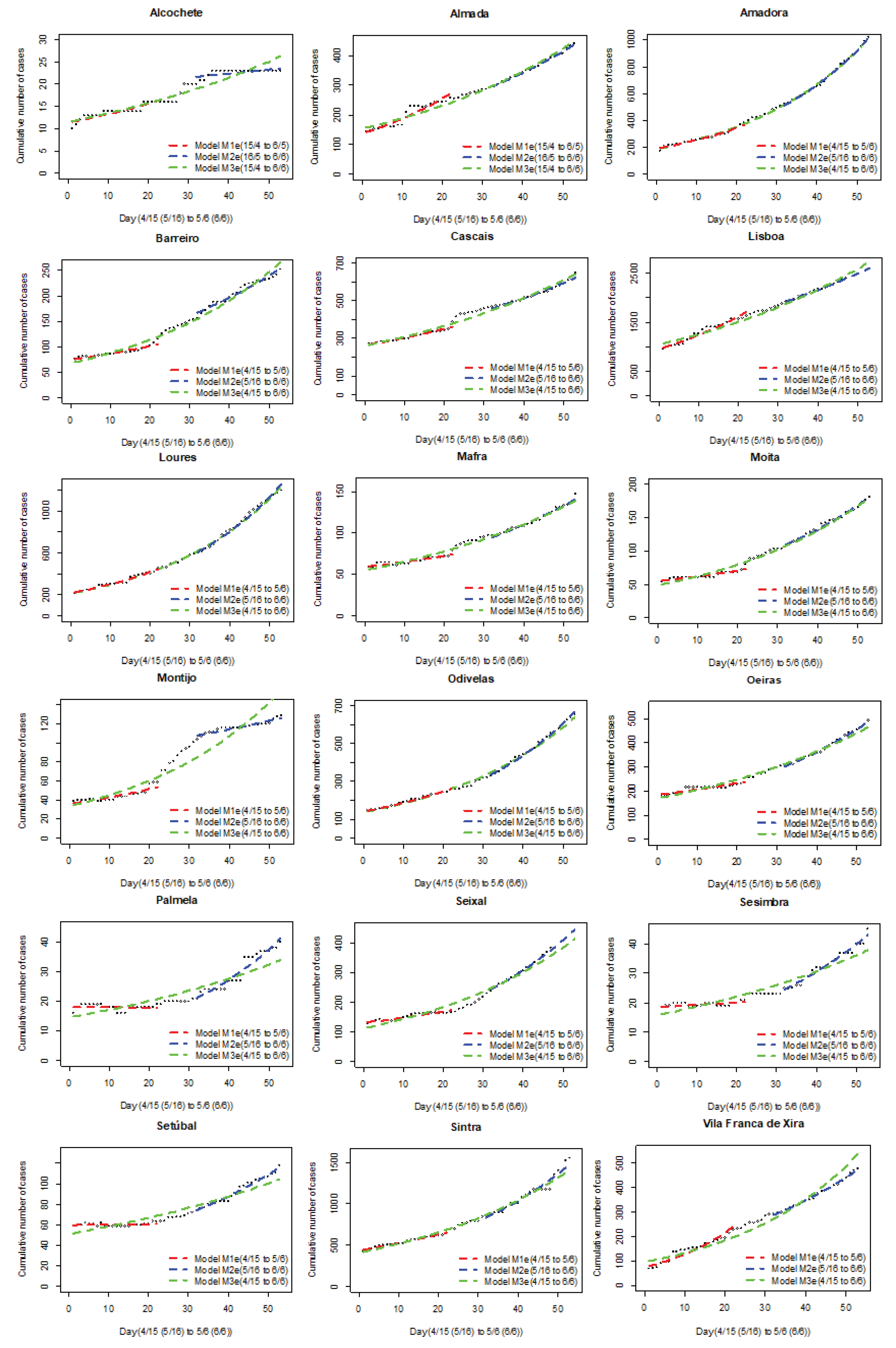
In Figure 4, we exemplify observed data and model fits for Periods S1 & S3. S2 reflects the ongoing case reporting dynamic of potential May 1st contagion for three counties (more in Appendix A). There are cases of regression lines being approximately parallel or clearly concurrent.

An One-Way ANCOVA test was applied to $M{3}_i$ models (models (9)), $i=1,2,\cdots ,18$, to test for each the following hypotheses:

$$H_{0AN{C}_i}:{\gamma }_i=0\mathit{versus}{H}_{1AN{C}_i}:{\gamma }_i\ne 0.$$

(10)

Table 2 shows results of the fit significance levels for linear models M1 and M2 (8) and for their slope homogeneity tests, for each county.

Besides evaluating slope differences of linear models, it is necessary to evaluate if significant differences result from a change in linear behaviour or simply reflect an exponential growth that was already underway. For that, exponential models were fitted to the data of each county for Periods S1 and S3. Furthermore, an exponential model (11) was fit to each county with all data (models $M3e_i,i=1,2,\cdots ,18$) and a model with interaction t × Dummy for period $S_1\cup S_3$ (models $M4e_i$ (12)) to test the coefficient homogeneity of t in models $M1e_i$ and $M2e_i$ (11) (similar hypotheses to the ones defined for linear models $M{1}_i$ and $M{2}_i$).

$$M1e_i,M2e_i,M3e_i:ln\left(NCase{s}_i\right)={\beta }_{0i}+{\beta }_{1i}t+{\epsilon }_i,\mathrm{with}{\epsilon }_i\sim N(0,{\sigma }^2)\mathrm{and}iid.$$

(11)

$$\begin{array}{c}\hfill M4e_i:ln\left(NCase{s}_i\right)={\beta }_{0i}+{\beta }_{1i}t+{\beta }_{3i}Dumm{y}_i+{\gamma }_{i}Dumm{y}_i+{\epsilon }_i\\ \hfill {\epsilon }_i\mathrm{s}\mathrm{are}iid\mathrm{and}{\epsilon }_i\sim N(0,{\sigma }^2),i=1,2,\cdots ,18.\end{array}$$

(12)

Three county graphs are displayed in Figure 5, with more in Appendix A.

Per the second stage, we visually inspect the models to identify counties in which there was a reduction in the rate of change of the cumulative number of cases or where the statistical difference resulted from a significant change within the S2 period, but the S1 and S3 models correspond to straight lines with very similar slopes.

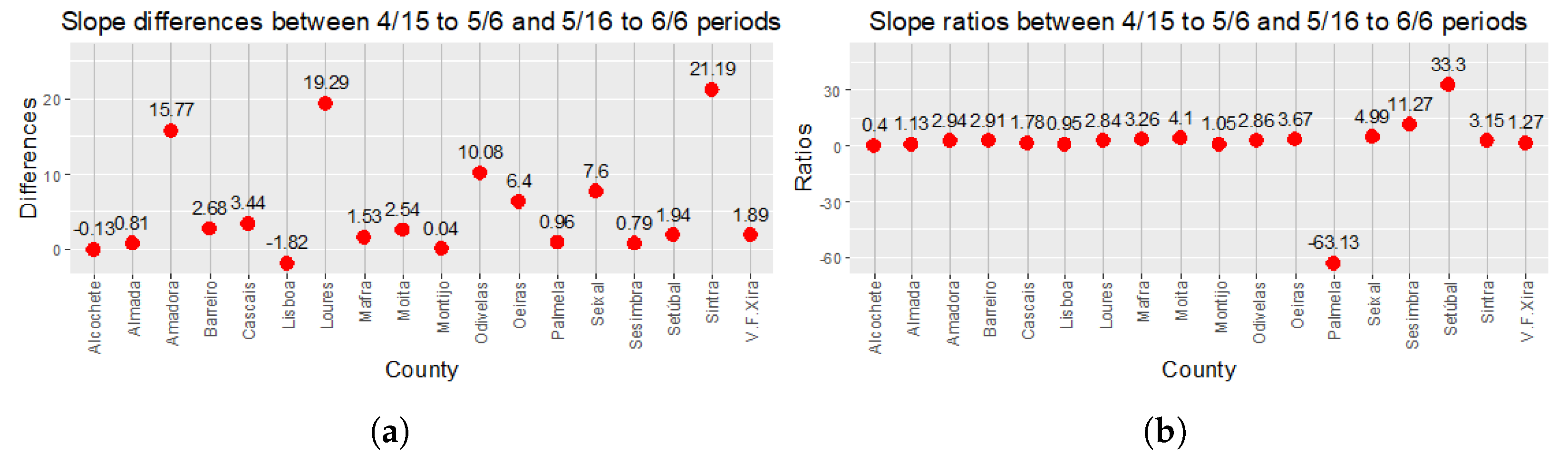
Per the third stage, we analyzed the linear and exponential behaviour of data and the nature of the differences. Figure 6 enables visual analysis of slope ratios (Figure 6a) of models M2 and M1 (Equation (5)), as well as their differences (Figure 6a). One can analyze both the proportions of estimated slopes and the magnitude of their differences. For example, the rate of change of Sesimbra for S1 is nearly eleven times greater than that for the S3 period. However, considering the value of the difference of change rates, these are necessarily less than 1. Further, on 6 June, the cumulative number of cases was only 45. For Loures, the ratio is near 3, and the difference is close to 19, therefore the rate of change underwent a very significant increase from S1 to S3. For counties in which the homogeneity of the slopes of the linear models was rejected, the ANCOVA test was used to test the homogeneity of the t coefficients of the exponential models.

Per stage four, for counties in which the hypothesis of homogeneity of slopes of the linear model was rejected but the homogeneity of the coefficients of the exponential term was not rejected, we evaluate whether linear or exponential models best fit to S1 and S3 data, comparing adjusted R-squared values and RMSE, for cases where both models were statistically significant, with at least 1% significance level (higher values, better fit:

Table 3. The p-values of F-statistics of the tests of the goodness-of-fit of the global models (linear—M1, M2 and exponential—M1e, M2e) for both periods, S1 and S3, the respective models adjusted R-squared and RMSE values.

	Adjusted R-Squared, RMSE and p Values of F Statistic for Linear/Exponential Models
	(S1 Period)						(S2 Period)
	R2 (M1)	R2 (M1e)	RMSE M1	RMSE M1e	p-Value (F Test M1)	p-Value (F Test M1e)	R2 (M2)	R2 (M2e)	RMSE (M2)	RMSE (M2e)	p-Value (F Test M2)	p-Value (F Test M2e)
Alcochete	0.8074	0.7979	0.6351	0.6518	8.3 $\times {10}^{-09}$	3.217 $\times {10}^{-08}$	0.392	0.3831	0.6302	0.6354	0.001	0.001156
Almada	0.8956	0.8811	12.690	13.594	1.742 $\times {10}^{-11}$	2.663 $\times {10}^{-11}$	0.9912	0.9960	3.9882	2.6733	2.2 $\times {10}^{-16}$	<2.2 $\times {10}^{-16}$
Amadora	0.948	0.9669	11.748	9.4032	1.604 $\times {10}^{-14}$	8.525 $\times {10}^{-16}$	0.9807	0.9965	20.728	9.0382	<2.2 $\times {10}^{-16}$	<2.2 $\times {10}^{-16}$
Barreiro	0.8438	0.8667	3.7153	3.4520	1.005 $\times {10}^{-09}$	5.496 $\times {10}^{-11}$	0.9696	0.9555	4.4700	5.4501	<2.2 $\times {10}^{-16}$	3.836 $\times {10}^{-15}$
Cascais	0.9206	0.9316	8.0431	7.4810	2.686 $\times {10}^{-16}$	4.848 $\times {10}^{-14}$	0.9586	0.9719	10.121	8.3874	<2.2 $\times {10}^{-16}$	<2.2 $\times {10}^{-16}$
Lisbon	0.9711	0.9517	36.220	47.396	<2.2 $\times {10}^{-16}$	2.251 $\times {10}^{-15}$	0.9971	0.9970	10.737	10.995	<2.2 $\times {10}^{-16}$	<2.2 $\times {10}^{-16}$
Loures	0.962	0.9699	12.863	11.443	6.897 $\times {10}^{-16}$	<2.2 $\times {10}^{-16}$	0.9953	0.9861	12.626	22.321	<2.2 $\times {10}^{-16}$	<2.2 $\times {10}^{-16}$
Mafra	0.7822	0.7937	2.2045	2.1473	2.881 $\times {10}^{-08}$	2.314 $\times {10}^{-08}$	0.9685	0.9810	2.4683	1.9282	<2.2 $\times {10}^{-16}$	<2.2 $\times {10}^{-16}$
Moita	0.8021	0.8166	2.5033	2.4144	1.095 $\times {10}^{-08}$	2.8 $\times {10}^{-09}$	0.9912	0.9896	1.9644	2.1375	<2.2 $\times {10}^{-16}$	<2.2 $\times {10}^{-16}$
Montijo	0.7301	0.7689	3.1501	2.9459	2.535 $\times {10}^{-07}$	6.508 $\times {10}^{-08}$	0.8869	0.8869	1.9533	1.9532	3.915 $\times {10}^{-11}$	4.384 $\times {10}^{-11}$
Odivelas	0.9906	0.9876	3.2683	3.7731	<2.2 $\times {10}^{-16}$	<2.2 $\times {10}^{-16}$	0.9944	0.9942	7.2217	7.4162	<2.2 $\times {10}^{-16}$	<2.2 $\times {10}^{-16}$
Oeiras	0.7640	0.7671	8.1939	8.3480	6.501 $\times {10}^{-08}$	6.38 $\times {10}^{-08}$	0.9839	0.9928	6.9605	4.6913	<2.2 $\times {10}^{-16}$	<2.2 $\times {10}^{-16}$
Palmela	−0.0406	−0.0405	1.0169	1.0173	0.6751	0.7163	0.9124	0.9145	1.8132	1.7920	2.984 $\times {10}^{-12}$	1.867 $\times {10}^{-12}$
Seixal	0.8745	0.8633	4.4538	4.6542	1.113 $\times {10}^{-10}$	1.735 $\times {10}^{-10}$	0.9929	0.9972	4.9610	3.1420	<2.2 $\times {10}^{-16}$	<2.2 $\times {10}^{-16}$
Sesimbra	0.2056	0.2049	0.8590	0.8598	0.01964	0.02118	0.9665	0.9661	0.9999	1.0073	<2.2 $\times {10}^{-16}$	<2.2 $\times {10}^{-16}$
Setúbal	0.0396	0.0406	1.2547	1.2541	0.5112	0.1905	0.9696	0.9726	2.1893	2.0761	1.105 $\times {10}^{-14}$	<2.2 $\times {10}^{-16}$
Sintra	0.9731	0.9703	10.155	10.696	<2.2 $\times {10}^{-16}$	<2.2 $\times {10}^{-16}$	0.9285	0.9511	53.297	44.389	3.926 $\times {10}^{-13}$	2.283 $\times {10}^{-15}$
Vila Franca de Xira	0.9542	0.9150	9.4361	13.733	4.448 $\times {10}^{-15}$	1.298 $\times {10}^{-11}$	0.981	0.9923	7.6275	4.8762	<2.2 $\times {10}^{-16}$	<2.2 $\times {10}^{-16}$

(1) Yellow color identifies the counties of Group 1. (2) Green color identifies the models with the best goodness-of-fit by the R² and RMSE criteria. (3) Red color identifies the counties in which the goodness-of-fit test is not significant at a significance level of 5%.

).

6. Results and Discussion

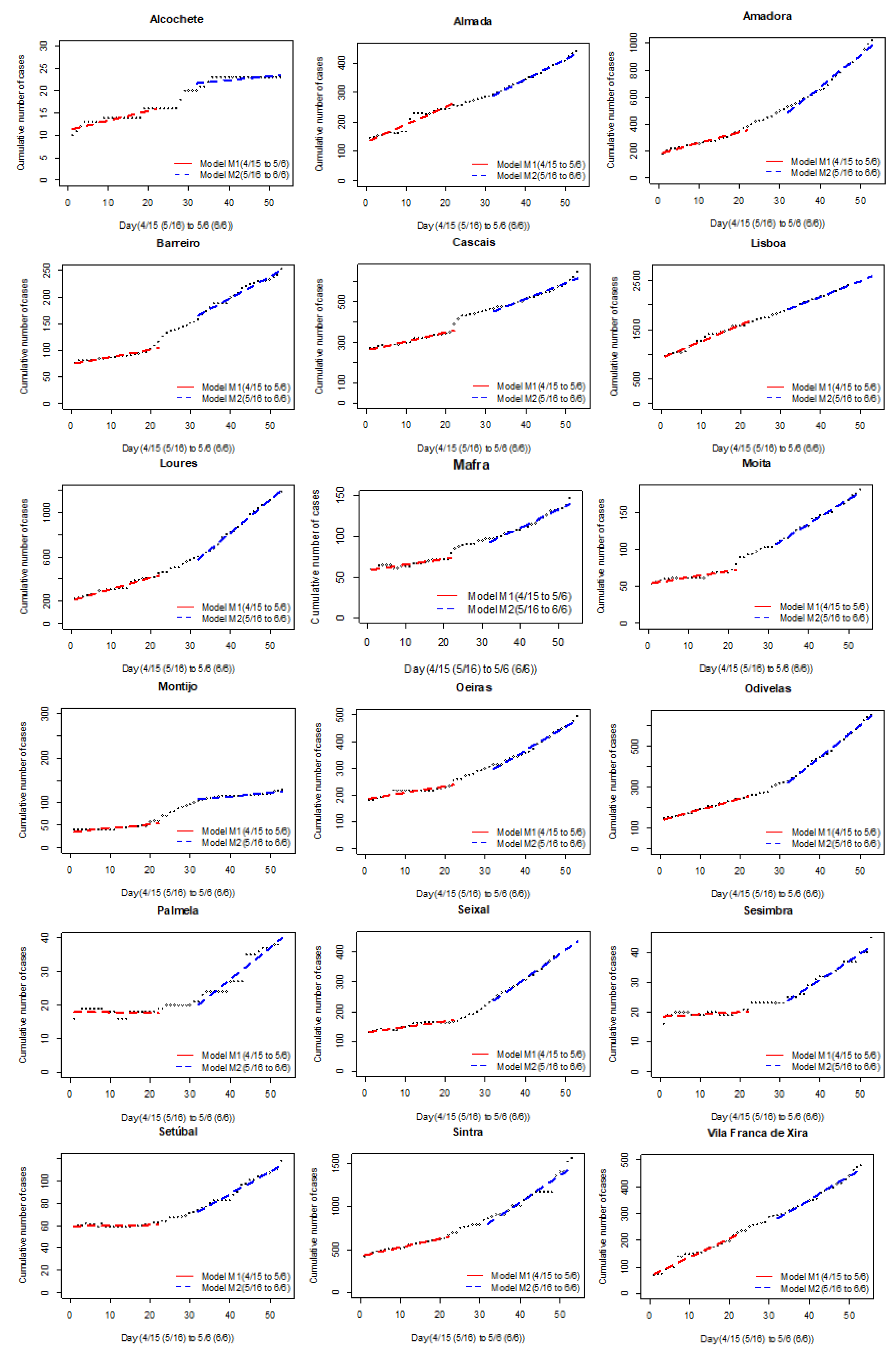
The method concluded for likely event impact with geographical heterogeneous effects in the AML region. Thus, one can analyze potential underlying mechanisms to support public discussion and policies. Here, we look at transportation as one avenue of analysis. In Group 1, of counties where, by hypothesis, the means of transportation used for travelling to the May 1st Demonstration location were the subway, or a combination of subway and train, with less than 60 min travel time, three situations stand out: (1) for the counties of Almada, Lisbon, and Vila Franca de Xira, the difference in rates of change of cumulative cases in both periods were not shown to be significant, and, at 5% level, one cannot reject that there was no significant change in the cases growth pattern between period S1 and period S3; (2) the counties of Amadora and Cascais exhibit significant change in growth rates, but when fitting for exponential models, the t variable coefficients do not register significant differences, at 5% significance level, and thus one cannot reject that the cases growth pattern did not change between those periods; and (3) counties of Odivelas, Oeiras, and Sintra present statistically significant differences in t variable coefficients, at 5% significance level, for both linear and exponential models, which leads to rejecting that the growth pattern is maintained over both periods.

For Group 2, of counties where, by hypothesis, the means of transportation used for travelling to the May 1st Demonstration location were chartered buses or private vehicles, there are also three situations that stand out: (1) Alcochete county, which exhibits a statistically significant difference in growth rates, at 5% significance level, reducing from period S1 to S3; (2) counties of Barreiro, Mafra, Moita, Palmela, Seixal, Sesimbra, and Setúbal, which present statistically significant differences in daily cases growth rates between both periods, as well as for t variable coefficients in exponential models (p-value $<0.005$)—thus leading us to reject the null hypothesis of there being no changes in the growth patterns from Period S1 to Period S3 in those counties. The county of Montijo exhibits the same behaviour regarding hypotheses testing results. 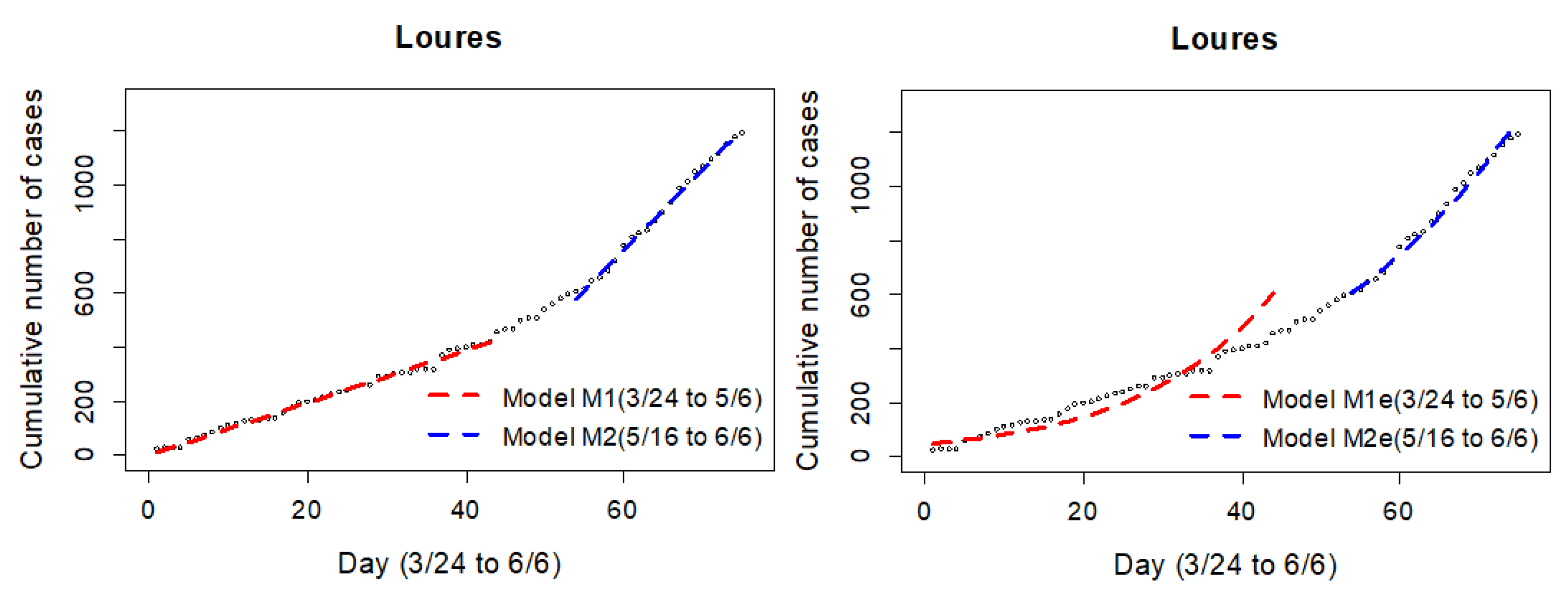However, graphic analysis of Figure 7 reveals that its growth behaviours in Periods S1 and S3 are identical (the ratio of growth rates is approximately 1, and their difference is approximately 0), and the hypotheses testing results are being impacted by a sudden spike of growth in period S2, without an overall impact in the growth pattern; and (3) Loures county exhibits a statistically significant difference in growth rates between both periods, at 5% significance level, but the exponential models do not present statistically significant differences in t variable coefficients, at the same significance level. One might infer that the exponential growth was already occurring prior, and that the growth rate for period S1 might have been underway. Using adjusted $R^2$ and RMSE values, however, reveals that, for the period S1, the exponential model has the best fit, whereas for the S3 period, the linear model has the best fit. Lacking an objective reason for this behavior (transitioning from slow exponential to fast linear), we questioned whether the exponential adjustment in the slower period (S1) might not simply be a misinterpretation of a linear period. To explore this possibility, the window of the S1 time period was extended, anticipating it to March 24, the first day that data for the counties are available. Over this extended window, the linear model provided the best fit (Figure 6), clarifying the anomaly. This county was then assigned to the category of counties potentially impacted by the event, as per the model with the best fit to the S1 (now extended) and S3 periods.

The same analysis was conducted for the counties of Amadora and Cascais. The exponential models are those with the greatest R-squared values for both periods, S1 and S3. Again, we confirmed the patterns by evaluating the same extended period for S1. As for Loures county, the best fit for this period was a linear model. However, unlike for Loures, for these counties, the best fit for S3 is an exponential model. A change in contagion pattern leading from linear to exponential is common in contagion dynamics and not confounding. Thus, we kept the decision taken based on the exponential models and did not reject the null hypothesis. The counties associated with the change in the growth pattern were those where likely means of travel to the demonstration were chartered buses or private cars, rather than subway or trains.

7. Considerations and Conclusions

In this work, we presented an empirical analysis method to assess, for events with superspreader contagion potential, the possibility of occurrence of geographically heterogeneous impacts. To exemplify it, we evaluated the potential impact of the May 1st Demonstration in Lisbon on the growth patterns of COVID-19 cases in AML counties in Portugal.

We analyzed the evolution of case growth between 15 April and 6 June, a period divided into series without expectable event impact, with potential partial event impact, and potential full event impact. We found a statistically significant change in the growth pattern of the overall geographic space (AML) between the period with no expectable influence of possible contagion due to the demonstration (15 April–6 May) and the period where any such influence would most certainly be visible (16 May–6 June). We also found a change in the growth pattern when considering cases for the same periods in the rest of the country. However, for AML, the growth accelerated from the first time period to the subsequent one, whereas, in the rest of the country, there was a deceleration, which was already discernible in the time period prior to the event. This change in the growth patterns supports the conclusion that there was a statistically significant impact from the event in AML contagion.

To assess which counties most contributed towards this change, we designed the empirical analysis methodology presented in this work. The methodology enabled concluding that the counties associated with the change in the growth pattern of the number of cases in AML were those where the means of transportation used to travel to the May 1st Demonstration were chartered buses or private cars, rather than subway or trains.

The method designed for this empirical study is innovative and sufficiently straightforward. It enables analysing potential geographically heterogeneous impact of an event in contagion dissemination by following a set of systematic steps. Its application to events subject to media controversy, such as Lisbon’s May 1st 2020, enables extracting well founded conclusions, as well as contributing to informed public discussion and decision-making, within a short time frame of the event occurring.

Besides the innovative method we presented, other more complicated mathematical models, e.g., an ensemble model that incorporates the generalized-growth model and the generalized logistic model, as proposed by [32], could also be useful to predict regional growth patterns of COVID-19 cases. Future work to improve the method may explore the effectiveness of using other statistical models, plausible models with the data, such as ensemble models refered above, Poisson regression models, classic logistic regression models, autoregressive integrated moving average (ARIMA) models, or artificial intelligence approaches, such as nonlinear autoregressive neural networks, adaptive neuro-fuzzy inference systems, hybrid fractal-fuzzy approaches, long short-term memory networks, Bayesian neural networks, or variational auto-encoder and singular spectrum analysis [2,33,34].

Identifying distinctive impact factors in the contagion rate can also inspire subsequent studies on actual contagion mechanisms that may explain it, thus contributing to adopting preventive or corrective measures for future events.