Energy Flow Analysis Model of High-Frequency Vibration Response for Plates with Free Layer Damping Treatment

Abstract

The energy flow analysis (EFA) model is developed for predicting the vibrational response of plates with free layer damping (FLD) treatment under high-frequency excitation. For the plate with fully free layer damping (FFLD) treatment, the energy density equation of the laminated plate with high damping is deduced by combining the equivalent complex stiffness method with the EFA theory. For the plate with partially free layer damping (PFLD) treatment, the relationship between energy density and energy intensity is obtained based on the wave theory of coupled plate by analyzing the energy transfer relationship at the damping boundary. The high-frequency energy density response of the structure with FLD treatment is solved through the energy finite element analysis (EFEA) method. To verify the developed EFEA model, several numerical analyses are performed for the plate with FFLD and PFLD treatments. The numerical results demonstrate that the obtained EFEA solutions consistently converge to the time-averaged modal analytical solutions at various analysis frequencies. Finally, the influences of the loss factor and the thickness of the damping layer on the resulting energy density are investigated in detail.

1. Introduction

Hypersonic aircrafts usually work in extreme noise environments with high-frequency- and high-sound-energy levels, the induced structural vibration of which will affect the normal operation of precision instruments in the cabin, and even cause damage to and the failure of the key electronic equipment [1,2,3]. Damping vibration attenuation technology can effectively control vibration and noise by laying a viscoelastic material layer on large-scale and thin-walled structures, so it is used in vibration and noise reduction in the bulkhead structures in hypersonic aircraft [4,5,6]. Therefore, the prediction and analysis of the dynamic characteristics for a thin-walled structure with free layer damping (FLD) treatment in the conceptual design stage has important theoretical and engineering value to realize the optimal design based on the acoustic and vibration performance.

In the aerospace field, the plate and shell structures are widely used in the dynamic modeling and analysis of thin-walled structures such as the fuselage and cabin in hypersonic aircraft. Xia et al. [6] established a vibration analysis model of a thin plate with FLD treatment based on the wave function method and proposed a modeling method for the three-dimensional coupled model of the FLD structure and the acoustic cavity. Liu et al. [7] investigated the bending vibration of thin plates under arbitrary boundary conditions considering the elastic and damping characteristics of the boundary. Hypersonic aircrafts are generally exposed to high-frequency acoustic and vibration environments induced by aerodynamic turbulence and noise, the mechanical behavior of which is characterized by short-wave high-frequency vibration. The above deterministic analysis method taking displacement as the basic variable is difficult to apply to high-frequency dynamic analysis due to the large calculation cost and the parameters’ sensitivity [8].

The high-frequency vibration analysis of aerospace structures generally adopts the statistical energy analysis (SEA) method with the average acoustic and vibration energy of the subsystem as the basic variable. Gupta et al. [9] analyzed the distribution of the high-frequency sound field in an aircraft cabin under turbulent excitation. Cherif et al. [10] predicted the acoustic transmission loss of the enclosed acoustic cavity in a cone shell. Poblet-Puig et al. [11] combined the spectral element method with the statistical energy method to establish the analysis model for the transmission loss of the L-shaped plate. Chen et al. [12,13] investigated the influence of the aspect ratio on the SEA parameters of the L-shaped plate in thermal environment. Hu et al. [14] modeled the effect of axial force on the coupling loss factor between beam structures. Based on the FE-SEA hybrid modeling technology, Gao et al. [15] proposed a design optimization method for the mid-frequency-vibration problem of plate–beam coupled structures. Zhang et al. [16] predicted the high-frequency vibration response of a line-coupled plate based on the transient SEA method. However, the SEA method can only give the average vibration response of the subsystem rather than that at any spatial position, such that the SEA method cannot accurately predict the high-frequency vibration response of the additional damping structure.

Different from the SEA method, the energy flow analysis (EFA) method, taking the energy density as the basic variable, can accurately predict the vibrational energy distribution within the subsystem. Zhang et al. [17] and Wang et al. [18] considered the temperature dependence of thermal stress and material parameters, and developed an EFA model for beam and plate structures under a uniform temperature field. However, their investigation neglected the effect of thermal stress on the energy density governing equation, which is important for the vibrational energy distribution as demonstrated in [19]. Yan et al. [20] used the energy finite element analysis (EFEA) method to investigate the numerical prediction method of high-frequency vibration of composite laminated structures. Liu et al. [21,22] established an EFA model of a functionally graded beam and analyzed the high-frequency vibration response in a thermal-gradient environment. Based on the equivalent fluid model, Yong et al. [23] proposed an EFA method for analyzing the propagation of compressional waves in porous media structures under high-frequency vibration. Cho et al. [24] presented an EFEA model of coupled structures by investigating the transformation and transferring characteristics of stress waves at the structural connection. Liu et al. [25] proposed an improved EFEA method by using the coupling loss factor to describe the power coupling relationship of the reverberation wave field between the coupled structures. Park et al. [26] developed an EFA model for the in-plane and out-of-plane vibrations of coupled Mindlin plates. Liu et al. [27] presented a low-noise topology optimization method for plate–beam coupled structures combining the EFEA method and the level set method. Yeo et al. [28] established an EFA model for pressure waves travelling in a three-dimensional elastic structure under high-frequency vibration. Zeng et al. [29] used EFA to predict the noise level of high-speed trains under the combined action of mechanical excitation and track noise excitation. Chen et al. [30] and Zhao et al. [31] proposed a method for predicting the transient response of structures under high-frequency impact loads based on the mixed EFEA method and virtual mode synthesis method. Chen et al. [32] investigated the high-frequency vibration of thin-plate structures in a supersonic airflow environment.

The above research is based on the assumption of small damping, where the energy density governing equation is derived using the wave number estimated by first-order approximation. However, this simplification produces significant errors in the high-frequency vibration response of structures with high damping loss factors. Han et al. [33,34] and Teng et al. [35] verified the above observation through the EFA for the one-dimensional system with high damping. Moreover, the conventional energy flow model is confined to uniform structures. In this paper, the plate with FLD treatment is a nonuniform structure with lamination and high damping, such that the traditional EFA method based on the assumption of small damping is no longer suitable in the prediction of the high-frequency vibration response for high-damping laminated plates. Therefore, it is necessary to develop an energy flow model for high-damping laminated plates without the low damping assumption.

In this study, the energy density governing equations for a laminated plate with free layer damping treatment were constructed without the low damping assumption. Through employing the exact wavenumber obtained, rather than its first-order approximation, the time–space-averaged energy density and intensity were calculated, which are regarded as the principal variables in the energy density governing equation. Unlike the traditional energy flow model, the developed energy flow model offers the relationship between time–space-averaged energy density and intensity with the absence of group velocity due to the large damping influence. Structural damping cannot be neglected as the potential energy and kinetic energy of the structure are significantly different. Thereby, the dissipated power was formulated by constructing the relationship between potential energy and total energy. The efficiency of the proposed energy flow model deduced without the low damping assumption was confirmed by comparing the results obtained from the developed energy flow model and the modal solutions for a plate with FFLD or PFLD treatment at high analysis frequencies.

The rest of this paper is organized as follows. In Section 2, the equivalent complex stiffness method is introduced to obtain the equivalent parameters such as the loss factor and Poisson ratio for a plate with FFLD treatment. Section 3 develops the energy density governing equation considering high damping effect and subsequentially establishes the corresponding EFEA model. In Section 4, wave transmission analysis is performed to obtain power transfer coefficients at a connection between the laminated and bare parts of a plate with PFLD treatment. Then, the energy density equation of the coupled plate is also solved. Section 4 verifies the presented EFA formulation by comparison between EFA solutions and modal solutions for various cases, and the influence of the damping layer parameters is discussed. In Section 5, the final conclusions are drawn.

2. Energy Flow Analysis Model for the Plate with FFLD Treatment

2.1. Equivalent Model of the Plate with FLD Treatment

Figure 1 is a plate with FFLD treatment under a concentrated harmonic load, where l_x and l_y are the length and width of the plate, respectively; h₁ and h₂ are the thickness of the metal layer and the damping layer, respectively. The concentrated harmonic load is applied to the point (x₀, y₀).

According to Kirchhoff’s thin-plate theory, the displacement fields of the plate with FLD treatment for transverse bending vibration in the x, y and z directions are expressed as

$$u(x,y,z)=-(z-z_0)\partial w(x,y)/\partial x$$

(1)

$$v(x,y,z)=-(z-z_0)\partial w(x,y)/\partial y$$

(2)

$$w(x,y)=w_0(x,y)$$

(3)

where z₀ is the position coordinate of the neutral plane.

According to Equations (1)–(3), the strain fields of the free damping plate $\mathit{\epsilon }={\left[\begin{array}{ccc}{\epsilon }_x& {\epsilon }_y& {\gamma }_{xy}\end{array}\right]}^{\mathrm{T}}$ are expressed as

$$\epsilon =(z-z_0)\kappa$$

(4)

where $\kappa ={\left[\begin{array}{lll}{\kappa }_x\hfill & {\kappa }_y\hfill & {\kappa }_{xy}\hfill \end{array}\right]}^{\mathrm{T}}$ is the curvature matrix: ${\kappa }_x=-{\partial }^{2}w/\partial x^2$, ${\kappa }_y=-{\partial }^{2}w/\partial y^2$, and ${\kappa }_{xy}=-2{\partial }^{2}w/\partial x\partial y$. The stress matrix of the metal layer and the damping layer is denoted by ${\sigma }^k={\left[\begin{array}{lll}{\sigma }_{xx}^k\hfill & {\sigma }_{yy}^k\hfill & {\tau }_{xy}^k\hfill \end{array}\right]}^{\mathrm{T}}$ (k = 1 for the metal layer and k = 2 for the free damping layer).

The stress–strain relationship of the structure under the condition of small deformation is formulated as

$${\sigma }^k={\mathit{Q}}^k\epsilon$$

(5)

$${\mathit{Q}}^k=Q_k\left[\begin{array}{ccc}1& v_k& 0\\ v_k& 1& 0\\ 0& 0& (1-v_k)/2\end{array}\right], Q_k=\frac{E_k}{1-v_k^2}$$

(6)

where $E_k$ and $v_k$ are the Young’s modulus and Poisson’s ratio of each layer, respectively, and ${\mathit{Q}}^k$ is the elastic matrix of each layer. The bending strain energy of the plate with FLD treatment is equal to the sum of the metal layer and free damping layer and written as

$$U=\frac{1}{2}{D}_{eq}{\displaystyle \underset{S}{\iint }{({\kappa }_x+{\kappa }_y)}^{2}dS}+D_{eqv}{\displaystyle \underset{S}{\iint }(-2{\kappa }_x{\kappa }_y+\frac{1}{2}{\kappa }_{xy}^2)dS}$$

(7)

$$D_{eq}={\displaystyle \sum _{k=1}^2{\displaystyle {\int }_{z_k}^{z_{k+1}}{Q}_k{(z-z_0)}^{2}dz}}$$

(8)

$$D_{eqv}=\frac{1}{2}{\displaystyle \sum _{k=1}^2{\displaystyle {\int }_{z_k}^{z_{k+1}}(1-v_k)Q_k{(z-z_0)}^{2}dz}}$$

(9)

where $D_{eq}$ and $D_{eqv}$ are the equivalent bending stiffness and torsional stiffness of the plate with FLD treatment and $h_1=z_2-z_1$ and $h_2=z_3-z_2$ are the thicknesses of the metal layer and damping layer, respectively.

The position coordinate of neutral plane z₀ can be solved from the following force balance equation along the x direction.

$$N_x={\displaystyle \sum _{k=1}^2{\displaystyle {\int }_{z_k}^{z_{k+1}}{\sigma }_x^{k}dz}}={\displaystyle \sum _{k=1}^2{\displaystyle {\int }_{z_k}^{z_{k+1}}{Q}_k(-\frac{{\partial }^{2}w}{\partial x^2})\cdot (z-z_0)dz}}=0$$

(10)

Thus, the position of neutral plane z₀ is written as

$$z_0=-\frac{Q_2{h}_2^2+2Q_1{h}_2{h}_1+Q_1{h}_1^2}{2Q_2{h}_2+2Q_1{h}_1}$$

(11)

To introduce the damping characteristics of the stiffness for the plate with FLD treatment, the equivalent complex stiffness of Equation (8) is rewritten as

$$D_{eq}^{*}={\displaystyle \sum _{k=1}^2{\displaystyle {\int }_{z_k}^{z_{k+1}}{Q}_k(1+\mathrm{j}{\eta }_k){(z-z_0)}^{2}dz}}$$

(12)

where ${\eta }_k$ is the loss factor of each layer. According, the equivalent loss factor of the plate with FLD treatment is expressed as

$${\eta }_{eq}=\frac{Im(D_{eq}^{*})}{Re(D_{eq}^{*})}=\frac{{\displaystyle \sum _{k=1}^2{\eta }_k{\displaystyle {\int }_{z_k}^{z_{k+1}}{Q}_k{(z-z_0)}^{2}dz}}}{{\displaystyle \sum _{k=1}^2{\displaystyle {\int }_{z_k}^{z_{k+1}}{Q}_k{(z-z_0)}^{2}dz}}}$$

(13)

In addition, the equivalent Poisson’s ratio of the plate with FLD treatment is obtained as

$$v_{eq}=1-\frac{2D_{eqv}}{D_{eq}}$$

(14)

2.2. Energy Density Equation of the FLD Plate

According to Hamilton’s law, the bending vibration equation of the plate with FLD treatment is

$$D_{eq}^{*}(\frac{{\partial }^{4}w}{\partial x^4}+2\frac{{\partial }^{4}w}{\partial x^2\partial y^2}+\frac{{\partial }^{4}w}{\partial y^4})+m_{eq}\frac{{\partial }^{2}w}{\partial t^2}=F_0\delta (x-x_0)\delta (y-y_0)e^{j\omega t}$$

(15)

where $m_{eq}={\rho }_1{h}_1+{\rho }_2{h}_2$ is the equivalent surface mass of the free damping plate (${\rho }_1$ and ${\rho }_2$ are the densities of the metal layer and the free damping layer, respectively), $F_0$ is the amplitude of the harmonic excitation, ω = 2πf is the circular frequency and $\delta (\cdot )$ is the Dirac function. The steady-state vibration solution of Equation (15) is defined as

$$w\left(x,y,t\right)=A{e}^{-\mathrm{j}(k_{x}x+k_{y}y)}{e}^{\mathrm{j}\omega t}$$

(16)

where $k_x=k_f\cos \phi$ and $k_y=k_f\sin \phi$ represent the bending wavenumber components in the x and y directions, respectively (φ is the scattering angle of the bending wave and k_f is the total bending wavenumber).

By substituting Equation (15) into Equation (13), the dispersion equation is obtained as

$$D_{eq}^{*}{k}_f^4-m_{eq}{\omega }^2=0$$

(17)

The bending wavenumber is calculated as

$$k_f=\pm \sqrt[4]{\frac{m_{eq}{\omega }^2}{D_{eq}^{\ast }}},\hspace{1em}\pm \mathrm{j}\sqrt[4]{\frac{m_{eq}{\omega }^2}{D_{eq}^{\ast }}}$$

(18)

According to the assumption of the reverberant wave field, the propagation direction of the bending wave is uncertain, so these wavenumber components are averaged in the range of the scattering angle [0, 2π] as

$${\overline{k}}_x=\sqrt{\frac{1}{2\pi }{\displaystyle {\int }_0^{2\pi }{[k_f\cos \phi ]}^2}d\phi }={\overline{k}}_{x1}+j{\overline{k}}_{x2}$$

(19)

$${\overline{k}}_y=\sqrt{\frac{1}{2\pi }{\displaystyle {\int }_0^{2\pi }{[k_f\sin \phi ]}^2}d\phi }={\overline{k}}_{y1}+j{\overline{k}}_{y2}$$

(20)

From the wave theory, the first two terms in Equation (18) correspond to the far-field waves oscillating in space, and the last two terms correspond to the near-field waves with exponentially decaying. For the high-frequency vibrating plate, the wavelength of the bending wave is much smaller than the in-plane size of the plate, and thereby the influence of the near-field waves is generally ignored in the EFA. Equation (16) is rewritten as

$$w_f(x,y,t)=\left(A_f{e}^{-\mathrm{j}{\overline{k}}_{x}x-\mathrm{j}{\overline{k}}_{y}y}+B_f{e}^{\mathrm{j}{\overline{k}}_{x}x-\mathrm{j}{\overline{k}}_{y}y}+C_f{e}^{-\mathrm{j}{\overline{k}}_{x}x+\mathrm{j}{\overline{k}}_{y}y}+D_f{e}^{\mathrm{j}{\overline{k}}_{x}x+\mathrm{j}{\overline{k}}_{y}y}\right)e^{\mathrm{j}\omega t}$$

(21)

where A_f, B_f, C_f and D_f represent the amplitude of each far-field wave.

In addition, the loss factor of the general metal structure is small, so the existing EFA theory is based on the low damping assumption, and the energy density equation is deduced by the first-order approximation of the wavenumber to the loss factor. However, the viscoelastic damping layer causes the high loss factor of the plate with FLD treatment such that the traditional energy flow analysis will bring significant errors [19,20]. In order to predict the high-frequency vibration response of the plate with FLD treatment accurately, the energy density equation is deduced by the exact wavenumber to modify the traditional EFA theory.

The time-averaged energy density of the thin plate structure in one vibration period $〈e〉$ consists of the kinetic energy density $〈e_k〉$ and the potential energy density $〈e_p〉$ [24,26].

$$〈e〉=〈e_k〉+〈e_p〉$$

(22)

where

$$〈e_k〉=\frac{1}{4}\mathrm{Re}\left[m_{eq}\frac{\partial w}{\partial t}{\left(\frac{\partial w}{\partial t}\right)}^{\ast }\right]$$

(23)

$$〈e_p〉=\frac{1}{4}\mathrm{Re}\left\{D_{eq}^{*}\left[\begin{array}{l}\frac{{\partial }^{2}w}{\partial x^2}{\left(\frac{{\partial }^{2}w}{\partial x^2}\right)}^{\ast }+2v_{eq}\frac{{\partial }^{2}w}{\partial x^2}{\left(\frac{{\partial }^{2}w}{\partial y^2}\right)}^{\ast }+\frac{{\partial }^{2}w}{\partial y^2}{\left(\frac{{\partial }^{2}w}{\partial y^2}\right)}^{\ast }\\ +2(1-v_{eq})\left(\frac{{\partial }^{2}w}{\partial x\partial y}\right){\left(\frac{{\partial }^{2}w}{\partial x\partial y}\right)}^{\ast }\end{array}\right]\right\}$$

(24)

where ${\left(\cdot \right)}^{\ast }$ represents the complex conjugate operation, and $\mathrm{Re}\left(\cdot \right)$ represents the function taking the real part of the complex number.

The components $〈I_x〉$ and $〈I_y〉$ of time-averaged energy intensity are expressed as [18,24,25,26].

$$〈I_x〉=\frac{1}{2}\mathrm{Re}\left[-Q_{xz}{\left(\frac{\partial w}{\partial t}\right)}^{\ast }+M_x{\left(\frac{{\partial }^{2}w}{\partial x\partial t}\right)}^{\ast }+M_{xy}{\left(\frac{{\partial }^{2}w}{\partial y\partial t}\right)}^{\ast }\right]$$

(25)

$$〈I_y〉=\frac{1}{2}\mathrm{Re}\left[-Q_{yz}{\left(\frac{\partial w}{\partial t}\right)}^{\ast }+M_y{\left(\frac{{\partial }^{2}w}{\partial y\partial t}\right)}^{\ast }+M_{yx}{\left(\frac{{\partial }^{2}w}{\partial x\partial t}\right)}^{\ast }\right]$$

(26)

The bending moments M_x and M_y, the torque M_xy and the shear forces Q_xz and Q_yz can be obtained on the basis of the bending vibration theory of thin plates. By substituting the far-field solutions of Equation (21) into Equations (23)–(26), and then performing local spatial averaging in a wavelength to eliminate the power flow owing to the traveling wave interference term, we obtain the time–space averaged energy density and energy intensity as

$$〈\overline{e}〉=\frac{1}{4}\mathrm{Re}\left\{D_{eq}^{*}\left[\begin{array}{l}{\overline{k}}_x^2{\overline{k}}_x^{{\ast }^2}+2v_{eq}{\overline{k}}_x^2{\overline{k}}_y^{{\ast }^2}+{\overline{k}}_y^2{\overline{k}}_y^{{\ast }^2}\\ +2(1-v_{eq}){\overline{k}}_x{\overline{k}}_y{\overline{k}}_x^{\ast }{\overline{k}}_y^{\ast }\end{array}\right]+m_{eq}{\omega }^2\right\}\cdot 〈++++〉$$

(27)

$$〈\overline{I_x}〉=-\frac{1}{2}\omega \mathrm{Re}\left\{D_{eq}^{*}\left[\begin{array}{l}{\overline{k}}_x^3+{\overline{k}}_x{\overline{k}}_y^2+{\overline{k}}_x^2{\overline{k}}_x^{\ast }+v_{eq}{\overline{k}}_y^2{\overline{k}}_x^{\ast }\\ +(1-v_{eq}){\overline{k}}_x{\overline{k}}_y{\overline{k}}_y^{\ast }\end{array}\right]\right\}\cdot 〈-+-+〉$$

(28)

$$〈\overline{I_y}〉=-\frac{1}{2}\omega \mathrm{Re}\left\{D_{eq}^{*}\left[\begin{array}{l}{\overline{k}}_x^3+{\overline{k}}_x^2{\overline{k}}_y+v_{eq}{\overline{k}}_x^2{\overline{k}}_y^{\ast }+{\overline{k}}_y^2{\overline{k}}_y^{\ast }\\ +(1-v_{eq}){\overline{k}}_x{\overline{k}}_y{\overline{k}}_x^{\ast }\end{array}\right]\right\}\cdot 〈--++〉$$

(29)

where $〈\pm \pm \pm \pm 〉=\pm {〈A〉}^{--}\pm {〈B〉}^{+-}\pm {〈C〉}^{-+}\pm {〈D〉}^{++}$.${〈A〉}^{\pm \pm }$ is expressed as

$${〈A〉}^{\pm \pm }=\frac{{\overline{k}}_x{\overline{k}}_y}{16{\pi }^2{\overline{k}}_{x2}{\overline{k}}_{y2}}{\left|A_f\right|}^2\left\{\begin{array}{l}\left[e^{\pm (-2{\overline{k}}_{x2}\pi /{\overline{k}}_x)}-e^{\pm (2{\overline{k}}_{x2}\pi /{\overline{k}}_x)}\right]\cdot \left[e^{\pm (-2{\overline{k}}_{y2}\pi /{\overline{k}}_y)}-e^{\pm (2{\overline{k}}_{y2}\pi /{\overline{k}}_y)}\right]\\ \cdot e^{\pm (-2{\overline{k}}_{x2}x)\pm (-2{\overline{k}}_{y2}y)}\end{array}\right\}$$

(30)

where ${\overline{k}}_{x2}$ and ${\overline{k}}_{y2}$ are the imaginary parts of wavenumbers ${\overline{k}}_x$ and ${\overline{k}}_y$, respectively. Comparing Equation (27) with Equations (28) and (29), there is the following relationship between the energy density and the energy intensity as

$$\begin{array}{cc}〈\overline{I_x}〉=\alpha \frac{\partial 〈\overline{e}〉}{\partial x}& 〈\overline{I_y}〉=\beta \frac{\partial 〈\overline{e}〉}{\partial y}\end{array}$$

(31)

where

$$\alpha =\frac{\omega \left[{\overline{k}}_x^3+{\overline{k}}_x{\overline{k}}_y^2+{\overline{k}}_x^2{\overline{k}}_x^{\ast }+v_{eq}{\overline{k}}_y^2{\overline{k}}_x^{\ast }+2(1-v_{eq}){\overline{k}}_x{\overline{k}}_y{\overline{k}}_y^{\ast }\right]}{{\overline{k}}_{x2}\left[{\overline{k}}_x^2{k}_x^{{\ast }^2}+2v_{eq}{\overline{k}}_x^2{\overline{k}}_y^{{\ast }^2}+{\overline{k}}_y^2{\overline{k}}_y^{{\ast }^2}+2(1-v_{eq}){\overline{k}}_x{\overline{k}}_y{\overline{k}}_x^{\ast }{\overline{k}}_y^{\ast }+m_{eq}{\omega }^2/D_{eq}^{*}\right]}$$

(32)

$$\beta =\frac{\omega \left[{\overline{k}}_x^3+{\overline{k}}_x^2{\overline{k}}_y+v_{eq}{\overline{k}}_x^2{\overline{k}}_y^{\ast }+{\overline{k}}_y^2{\overline{k}}_y^{\ast }+2(1-v_{eq}){\overline{k}}_x{\overline{k}}_y{\tilde{k}}_x^{\ast }\right]}{{\overline{k}}_{y2}\left[{\overline{k}}_x^2{\overline{k}}_x^{{\ast }^2}+2v_{eq}{\overline{k}}_x^2{\overline{k}}_y^{{\ast }^2}+{\overline{k}}_y^2{\overline{k}}_y^{{\ast }^2}+2(1-v_{eq}){\overline{k}}_x{\overline{k}}_y{\overline{k}}_x^{\ast }{\overline{k}}_y^{\ast }+m_{eq}{\omega }^2/D_{eq}^{*}\right]}$$

(33)

Additionally, the power balance equation can be expressed as [20,24].

$$〈\overline{{\pi }_{in}}〉=〈\overline{{\pi }_{diss}}〉+\nabla \cdot 〈\overline{\mathit{I}}〉$$

(34)

where $\nabla \cdot 〈\overline{\mathit{I}}〉=\partial 〈\overline{I_x}〉/\partial x+\partial 〈\overline{I_y}〉/\partial y$ represents the divergence operation on the energy intensity vector $〈\overline{\mathit{I}}〉=\left[\begin{array}{cc}〈\overline{I_x}〉& 〈\overline{I_y}〉\end{array}\right]$.

The average dissipated power of the laminated plate is related to frequency ω, structural loss factor $\eta$ and potential energy density $〈\overline{e_p}〉$, and can be formulated as [20,24].

$$〈\overline{{\pi }_{diss}}〉=2\eta \omega 〈\overline{e_p}〉$$

(35)

Combining Equation (24), Equation (27) and Equation (35), the average dissipated power of the plate with FFLD treatment is expressed as

$$〈\overline{{\pi }_{diss}}〉=2{\eta }_{eq}\omega 〈\overline{e_p}〉=\gamma 〈\overline{e}〉$$

(36)

$$\gamma =2{\eta }_{eq}\omega \frac{{\overline{k}}_x^2{\overline{k}}_x^{{\ast }^2}+2v_{eq}{\overline{k}}_x^2{\overline{k}}_y^{{\ast }^2}+{\overline{k}}_y^2{\overline{k}}_y^{{\ast }^2}+2(1-v_{eq}){\overline{k}}_x{\overline{k}}_y{\overline{k}}_x^{\ast }{\overline{k}}_y^{\ast }}{{\overline{k}}_x^2{\overline{k}}_x^{{\ast }^2}+2v_{eq}{\overline{k}}_x^2{\overline{k}}_y^{{\ast }^2}+{\overline{k}}_y^2{\overline{k}}_y^{{\ast }^2}+2(1-v_{eq}){\overline{k}}_x{\overline{k}}_y{\overline{k}}_x^{\ast }{\overline{k}}_y^{\ast }+m_{eq}{\omega }^2/D_{eq}^{*}}$$

(37)

Using the infinite admittance method [18,24], the average input power $〈{\overline{\pi }}_{in}〉$ is expressed as

$$〈{\overline{\pi }}_{in}〉=\frac{1}{2}{\left|F_0\right|}^2\mathrm{Re}\left(\frac{k_f^2}{8m_{eq}\omega }\right)$$

(38)

Substituting Equation (31), Equation (36) and Equation (38) into Equation (34), the energy density equation of the plate with FLD treatment is expressed as

$$\alpha \frac{{\partial }^2〈\overline{e}〉}{\partial x^2}+\beta \frac{{\partial }^2〈\overline{e}〉}{\partial y^2}+\gamma 〈\overline{e}〉=〈{\overline{\pi }}_{in}〉\delta (x-x_0)\delta (y-y_0)$$

(39)

We obtain Equation (39) by considering the high damping of the plate with FFLD treatment, using exact wavenumber instead without low damping assumption. Therefore, it can be used to predict the high-frequency vibration response of the plate with high damping.

To obtain the energy density, the finite element method is employed to solve Equation (39). We have

$${\mathit{K}}^e{\mathit{e}}^e={\mathit{F}}^e+{\mathit{Q}}^e$$

(40)

$${\mathit{K}}^e=-\frac{\alpha b}{6a}\left[\begin{array}{cccc}2& -2& -1& 1\\ -2& 2& 1& -1\\ -1& 1& 2& -2\\ 1& -1& -2& 2\end{array}\right]-\frac{\beta a}{6b}\left[\begin{array}{cccc}2& 1& -1& -2\\ 1& 2& -2& -1\\ -1& -2& 2& 1\\ -2& -1& 1& 2\end{array}\right]+\frac{\gamma ab}{9}\left[\begin{array}{cccc}4& 2& 1& 2\\ 2& 4& 2& 1\\ 1& 2& 4& 2\\ 2& 1& 2& 4\end{array}\right]$$

(41)

$${\mathit{F}}^e={\displaystyle {\int }_{{\Omega }^e}{\mathit{N}}^{\mathrm{T}}〈\overline{{\pi }_{in}}〉}\delta (x-x_0)\delta (y-y_0)d{\Omega }^e={\left.〈\overline{{\pi }_{in}}〉{\mathit{N}}^{\mathrm{T}}\right|}_{x=x_0,y=y_0}$$

(42)

$${\mathit{Q}}^e={\displaystyle {\oint }_{{\Gamma }^e}{\mathit{N}}^{\mathrm{T}}〈\overline{\mathit{I}}〉\cdot \mathit{n}}d{\Gamma }^e$$

(43)

where ${\mathit{K}}^e$ is the elemental stiffness matrix, ${\mathit{F}}^e$ is the elemental input power matrix, N is the shape function matrix with a 4-node bilinear quadrilateral element, ${\mathit{Q}}^e$ is the energy flow across the boundary, where the energy density is the discontinuous flux matrix, and ${\mathit{e}}^e$ is the elemental energy density matrix, parameters a and b are the respective halves of elemental length and width.

3. Energy Flow Analysis Model for the Plate with PFLD Treatment

In engineering, additional damping layers are often laid in severe vibration areas. Therefore, the energy flow analysis model of the plate with partial free layer damping treatment is constructed in this section. Figure 2 shows a plate with PFLD treatment under a concentrated harmonic load, divided into subdomains ① and ② at the damping boundary x = l_r. As the bending wave is incident at the damping boundary, the difference of the wave numbers in the two subdomains will cause the reflection and transmission of bending waves. Therefore, the plate with PFLD treatment can be equivalent to a coupled plate structure with different physical parameters.

Figure 3 is the power transmission relation between subdomains with and without free layer damping treatment. $q_f^{i+}$ $q_f^{i-}$(i = 1, 2) are energy intensity of bending waves, where superscript “+” denotes the right travelling wave and superscript “-” denotes the left travelling wave. ${\overline{\tau }}_{ffmn}$ (m, n = 1, 2) represents the energy transmission coefficient of the bending wave in subdomain m travelling into subdomain n at the damping boundary, ${\overline{\tau }}_{ffmm}$ represents the energy reflection coefficient at the damping boundary. According to the energy conservation law, the energy intensities satisfy the following relation.

$${〈{\overline{q}}_f^1〉}^{-}={\overline{\tau }}_{ff11}{〈{\overline{q}}_f^1〉}^{+}+{\overline{\tau }}_{ff21}{〈{\overline{q}}_f^2〉}^{-}$$

(44)

$${〈{\overline{q}}_f^2〉}^{+}={\overline{\tau }}_{ff12}{〈{\overline{q}}_f^1〉}^{+}+{\overline{\tau }}_{ff22}{〈{\overline{q}}_f^2〉}^{-}$$

(45)

The net energy intensity of travelling waves in subdomains ① and ② is expressed as

$$〈{\overline{q}}_f^1〉={〈{\overline{q}}_f^1〉}^{+}-{〈{\overline{q}}_f^1〉}^{\_}$$

(46)

$$〈{\overline{q}}_f^2〉={〈{\overline{q}}_f^2〉}^{+}-{〈{\overline{q}}_f^2〉}^{\_}$$

(47)

The energy density and energy intensity of travelling waves in subdomains ① and ② satisfy the following relationship as

$${〈{\overline{q}}_f^1〉}^{\pm }={\overline{c}}_{gf1}{〈{\overline{e}}_f^1〉}^{\pm }$$

(48)

$${〈{\overline{q}}_f^2〉}^{\pm }={\overline{c}}_{gf2}{〈{\overline{e}}_f^2〉}^{\pm }$$

(49)

where c_gfi is the group velocity of the bending waves in the subdomain i, and ${\overline{e}}_f^i$ is the energy density in the subdomain i. The group velocity characterizes the transfer velocity of the far-field elastic wave, which is obtained by deriving the implicit function about the wavenumber through the dispersion Equation (17).

$$c_{gfi}=\left|\frac{\partial \omega }{\partial k_{fi}}\right|=\left|\frac{2k_{fi}^3{D}_{eq}^{*}}{m_{eqi}\omega }\right|$$

(50)

The net energy density of travelling waves in subdomains ① and ② is expressed as

$$〈{\overline{e}}_f^1〉={〈{\overline{e}}_f^1〉}^{-}+{〈{\overline{e}}_f^1〉}^{+}$$

(51)

$$〈{\overline{e}}_f^2〉={〈{\overline{e}}_f^2〉}^{-}+{〈{\overline{e}}_f^2〉}^{+}$$

(52)

By combining Equations (44)–(52), the relationship between the energy intensity and the energy intensity at the damping boundary is obtained as

$$\left[\begin{array}{l}〈{\overline{q}}_f^1〉\hfill \\ 〈{\overline{q}}_f^2〉\hfill \end{array}\right]=\frac{{\overline{\tau }}_{ff12}}{2{\overline{\tau }}_{ff11}}\left[\begin{array}{ll}{\overline{c}}_{g1}\hfill & -{\overline{c}}_{g2}\hfill \\ -{\overline{c}}_{g1}\hfill & {\overline{c}}_{g2}\hfill \end{array}\right]\left[\begin{array}{l}〈{\overline{e}}_f^1〉\hfill \\ 〈{\overline{e}}_f^2〉\hfill \end{array}\right]$$

(53)

From Cho [24], the energy transmission coefficient and reflection coefficient can be obtained by solving the displacement continuity equation and mechanical equilibrium equation at the damping boundary followed by the obtained element stiffness matrix.

4. Verification and Discussion

In order to verify the established EFA model, the plates with FFLD and PFLD treatment simply supported on four edges are used as the benchmark examples. To obtain consistent results for the “exact” analytical solution, at least n = 500 terms of the expanded series are required using the modal method.

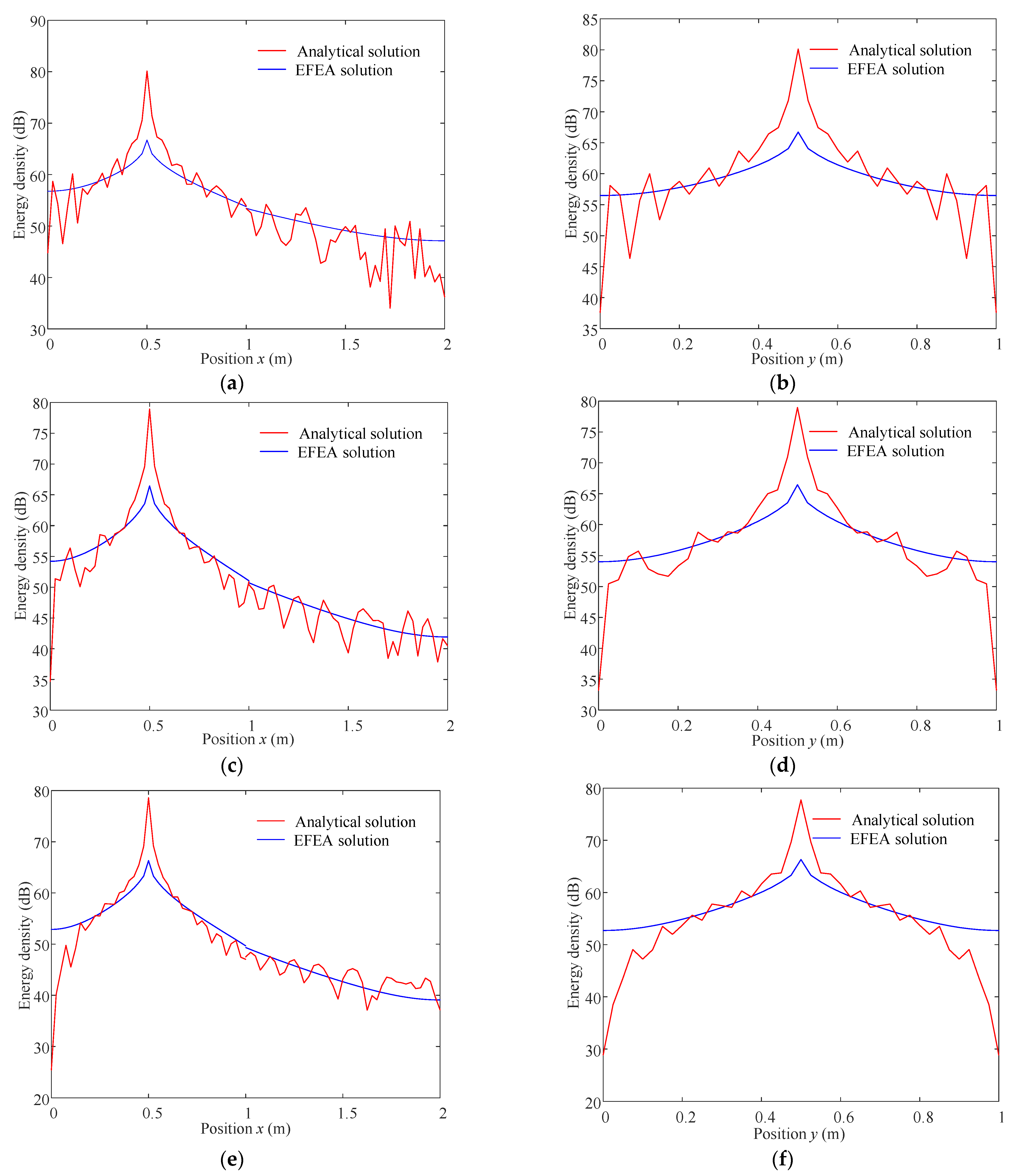
4.1. Plate with FFLD Treatment

As illustrated in Figure 1, the metal layer is made of aluminum alloy, which has the following dimensions and material properties: l_x × l_y × h₁ = 1 m × 1 m × 0.003 m, E₁ = 72 GPa, v₁ = 0.33, ρ₁ = 2700 kg/m³, η₁ = 0.05. The damping layer is made of rubber, whose dimensions and material properties are as follows: l_x × l_y × h₂ = 1 m × 1 m × (0.001~0.005) m, E₂ = 0.33 GPa, v₂ = 0.44, ρ₂ = 980 kg/m³, η₂ = 0.1~1. This plate with FFLD treatment is simply supported at four edges and subjected to a flexural harmonic force at the center (x₀ = 0.5 m, y₀ = 0.5 m), with the magnitude of F₀ = 1N and the frequency of f = 3 k~10 kHz.

The energy density was calculated by EFEA and modal methods in the various frequencies of 3 k, 5 k, 8 k and 10 kHz. These results, as shown in Figure 4 and Figure 5, were obtained employing the same parameters of damping layer: η₂ = 0.8, h₂ = 0.002 m. The time-averaged modal solutions exhibit the characteristic fluctuating behavior, while the EFEA solutions smoothly represent the global trend in the time-averaged modal solutions. This behavior demonstrates an expected match between displacement-based (modal method) and energy-based (EFEA) approaches. This consistency is good except for the neighborhood of the load application point and the boundaries, since the evanescent wave is ignored in the proposed EFEA model. The consistency errors in the load application point and the boundaries decrease with increasing excitation frequency. This is attributed to the fact that the wavelength becomes shorter, as depicted in Figure 6, such that the influence of the near-field wave is gradually reduced.

Figure 7 shows the energy density distribution for various loss factors of the damping layer with the thickness h₂ = 0.002 m in the frequency f = 3 kHz. From Equation (36), under the same input power and excitation frequency, the overall energy density is inversely proportional to the loss factor. Therefore, the global variation in energy density increases with larger damping. Figure 8 shows the energy density distribution for various thicknesses of the damping layer with a loss factor η₂ = 0.8 in the frequency f = 3 kHz. Similar to the loss factor, the large damping layer thickness causes significant energy dissipation, which leads to a relatively dramatic attenuation in the energy density.

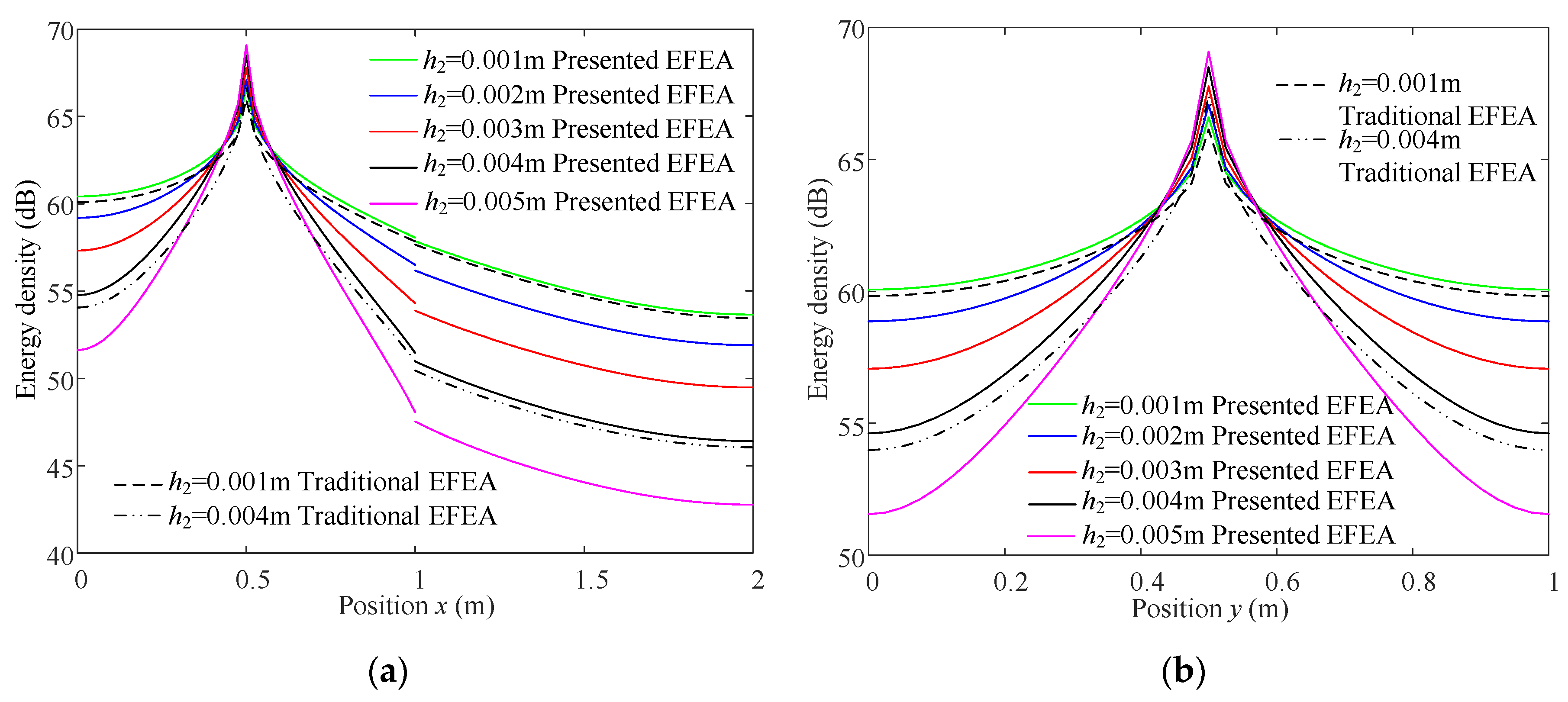
4.2. Plate with PFLD Treatment

In this example, this plate with PFLD treatment shares the same material properties as the plate with FFLD treatment in the first example. The dimensions of the metal layer and damping layer are as follows: l_x × l_y × h₁ = 2 m × 1 m × 0.003 m, l_x × l_y × h₂ = 2 m × 1 m × (0.001~0.005) m. The plate with PFLD treatment is excited by a flexural harmonic force at the point (x₀ = 0.5 m, y₀ = 0.5 m) with an amplitude of F₀ = 1N and a frequency of f = 3 k~10 kHz.

Figure 9 compares the energy densities between the EFEA and modal analytical method along one line aligned with the x-direction at x₀ = 0.5 m and the other with y-direction at y₀ = 0.5 m. These results are computed at the frequency f = 3 kHz with loss factor η₂ = 0.8 and thickness h₂ = 0.003 m of the damping layer. As expected, the EFEM results seem to converge to the time-averaged modal analytical solution. This observation is further confirmed through the obtained EFEM results under various excitation frequencies, as indicated in Figure 10.

Different from the plate with FFLD treatment, the energy density jump occurs due to the discontinuity of the material and thickness dimension at the damping boundary, as plotted in Figure 9 and Figure 10. This discontinuity results from the joint matrix (Equation (53)) and jumps as high as the group speed difference at the damping interface. Based on this point, both a large loss factor and thickness of the damping layer lead to a slight increase in the jump of energy density at the damping interface, as demonstrated in Figure 11 and Figure 12. In addition, the energy density more pronouncedly attenuates from the driving point to boundaries due to more damping dissipation, and thereby the overall energy density level is significantly reduced.

Additionally, the developed EFEA solutions are larger than the traditional EFEA solutions. The group velocities of the vibrating laminated plate in the developed energy flow model and the traditional energy flow model are formulated as

$$c_{gf}=\left|\frac{2k_f^3{D}_{eq}^{*}}{m_{eq}\omega }\right|=2{\omega }^{1/2}{m}_{eq}^{-1/4}{\left|D_{eq}^{*}\right|}^{1/4}$$

(54)

$$c_{gf,t}=\left|\frac{2\mathrm{Re}\left(k_f^3\right)\mathrm{Re}\left(D_{eq}^{*}\right)}{m_{eq}\omega }\right|=2{\omega }^{1/2}{m}_{eq}^{-1/4}{\left[\mathrm{Re}\left(D_{eq}^{*}\right)\right]}^{1/4}$$

(55)

where $c_{gf}$ denotes the group velocity in the presented EFEA model and $c_{gf,t}$ denotes the group velocity in the traditional EFEA model. Obviously, the former obtained from the exact wavenumber is higher than the latter obtained from the linear approximation of the exact wavenumber. Therefore, the energy density in the presented EFEA model is almost the same as that in the traditional EFEA model with a low damping assumption for a lightly damped system, as indicated in Figure 11. For a highly damped system, the reductions in the energy density in the proposed EFEA model are less than the counterpart in the traditional EFEA model, as indicated in Figure 11 and Figure 12. In general, the proposed EFEA model can efficiently predict the energy density distribution of the laminated plate at high frequency ranges regardless of whether it is a lightly or highly damped system.

5. Conclusions

In this paper, the energy density governing equation for a plate with FFLD or PFLD treatment is developed without low damping assumption. Different from the conventional energy flow model, which is exclusively fit for lightly damped uniform structures, the proposed energy flow model can predict the energy density of the laminated plate over low-to-high damping ranges. The developed energy flow model formulates the energy density governing equation by deriving the energy transfer equation and the power dissipation equation, which are obtained using the exact wavenumber without an approximation of its imaginary term. For a low damping system, the developed and traditional energy flow models have consistent energy density solutions due to the same wavenumbers and group velocities.

To verify the developed energy flow model, several energy flow analyses are performed for a plate with FFLD and PFLD treatment simply supported on all the four edges, and the obtained EFEA solutions are in contrast to the modal solutions and the conventional EFEA solutions. The numerical results demonstrate that the developed EFEA results provide greatly smooth representations of time-averaged modal solutions at various analysis frequencies. Particularly for a highly damped laminated plate, the energy density in the developed EFEA model is more favorable to propagate than that in the traditional EFEA model since the former has a higher group velocity than the latter. Consequently, the developed EFEA model inherently produces the accurate energy density regardless of the lightly or highly damped laminated plate at high frequency ranges.

Additionally, with the increasing loss factor and thickness of the free damping layer, the energy dissipation effect is enhanced such that the energy density level for the plate with FLD treatment reduces. However, compared with the loss factor, the thickness of the damping layer seems to generate more vibrational attenuation according to the energy density distribution.

High-frequency impact load generally occurs in aerospace engineering fields such as missile launches and spacecraft interstage separation. Thus, it is significant to develop an efficient analysis method to investigate the transient behavior of laminated plates subject to high-frequency impact load. In future study, the proposed EFEA method hybridizes the virtual mode synthesis and simulation (VMSS) method to predict the transient response of laminated structures under high-frequency impact load.

References

1. Zhao, H.D.; Hao, Z.W.; Liu, W.; Ding, J.F.; Sun, Y.; Zhang, Q.H.; Liu, Y.Z. The shock environment prediction of satellite in the process of satellite-rocket separation. Acta Astronaut. 2019, 159, 112–122. [Google Scholar] [CrossRef]
2. Wang, H.Z.; Yu, K.P.; Zhang, Z.Q.; Zeng, Y.X.; Wang, X. Prediction of the acoustic-vibration environment of an instrument cabin by using the energy finite element method. J. Vib. Shock. 2019, 38, 143–148. [Google Scholar]
3. Zhao, H.D.; Ding, J.F.; Hao, Z.W.; Liu, W.; Sun, Y.; Liu, Y.Z. Study on prediction methods of pyroshock environment for complex spacecraft structures. J. Aircr. 2020, 41, 35–43. [Google Scholar]
4. Yilmaz, I.; Arslan, E.; Cavdar, K. Experimental and numerical investigation of sound radiation from thin metal plates with different thickness values of free layer damping layers. Acoust. Austa. 2021, 49, 1–14. [Google Scholar] [CrossRef]
5. Shokrieh, M.M.; Najafi, A. Damping characterization and viscoelastic behavior of laminated polymer matrix composites using a modified classical lamination theory. Exp. Mech. 2007, 47, 831–839. [Google Scholar] [CrossRef]
6. Xia, X.J.; Xu, Z.M.; Lai, S.Y.; Zhang, Z.F.; He, Y.S. Responses of unconstrained damped vibro-acoustic systems using the wave based prediction technique. J. Vib. Shock. 2017, 36, 158–163. [Google Scholar]
7. Liu, L.; Cooradi, R.; Ripamonti, F.; Rao, Z.S. Wave based method for flexural vibration of thin plate with general elastically restrained edges. J. Sound Vib. 2020, 483, 115468. [Google Scholar] [CrossRef]
8. Petrone, G.; Melillo, G.; Laudiero, A.; De Rosa, S. A Statistical Energy Analysis (SEA) model of a fuselage section for the prediction of the internal Sound Pressure Level (SPL) at cruise flight conditions. Aerosp. Sci. Technol. 2019, 88, 340–349. [Google Scholar] [CrossRef]
9. Gupta, P.; Parey, A. Prediction of sound transmission loss of cylindrical acoustic enclosure using statistical energy analysis and its experimental validation. J. Vib. Control 2022, 151, 544. [Google Scholar] [CrossRef] [PubMed]
10. Cherif, R.; Wareing, A.; Atalla, N. Sound transmission paths through a statistical energy analysis model of mechanically linked aircraft double-walls. Noise Control Eng. J. 2020, 69, 411–421. [Google Scholar] [CrossRef]
11. Poblet-Puig, J. Estimation of the coupling loss factors of structural junctions with in-plane waves by means of the inverse statistical energy analysis problem. J. Sound Vib. 2021, 493, 133–145. [Google Scholar] [CrossRef]
12. Chen, Q.; Fei, Q.G.; Li, Y.B.; Wu, S.Q.; Zhang, P. Prediction of statistical energy analysis parameters in thermal environment. J. Spacecraft. Rockets 2019, 56, 687–694. [Google Scholar] [CrossRef]
13. Chen, Q.; Zhang, P.; Li, Y.B.; Wu, S.Q.; Fei, Q.G. Effect of aspect ratio on statistical energy analysis parameters of L-shaped folded plate under thermal environment. J. Vib. Shock. 2018, 37, 191–196. [Google Scholar]
14. Hu, W.L.; Chen, H.B.; Zhong, Q. Effects of axial force on coupling loss factor of beam structures. J. Vib. Shock. 2020, 39, 24–30. [Google Scholar]
15. Gao, R.X.; Zhang, Y.H.; Kenndy, D. Optimization of mid-frequency vibration for complex built-up systems using the hybrid finite element-statistical energy analysis method. Eng. Optim. 2019, 2019, 1691546. [Google Scholar] [CrossRef]
16. Zhang, L.; Li, X.H. Prediction of transient high-frequency vibration response of line-coupled plates. Acta Acust. 2018, 43, 61–68. [Google Scholar]
17. Zhang, W.B.; Chen, H.L.; Zhu, D.H.; Kong, X.J. The thermal effects on high-frequency vibration of beams using energy flow analysis. J. Sound Vib. 2014, 333, 2588–2600. [Google Scholar] [CrossRef]
18. Wang, D.; Xie, M.X.; Li, Y.M. High-frequency dynamic analysis of plates in thermal environments based on energy finite element method. Shock. Vib. 2015, 2015, 157208. [Google Scholar] [CrossRef] [Green Version]
19. Chen, Z.L.; Yang, Z.C.; Guo, N.; Zheng, G.W. An energy finite element method for high frequency vibration analysis of beams with axial force. Appl. Math. Model. 2018, 61, 521–539. [Google Scholar] [CrossRef]
20. Yan, X.Y. Energy Finite Element Analysis Developments for High Frequency Vibration Analysis of Composite Structures. Ph.D. Thesis, University of Michigan, Ann Arbor, MI, USA, 2008. [Google Scholar]
21. Liu, Z.H.; Niu, J.C. Vibrational energy flow model for functionally graded beams. Compos. Struct. 2018, 186, 17–28. [Google Scholar] [CrossRef]
22. Liu, Z.H.; Niu, J.C.; Jia, R.H. Vibrational energy flow model for high-frequency vibration of beams in thermal-gradient environment. CJA 2022, 43, 592–604. [Google Scholar]
23. Yong, H.K.; June, Y.K. Energy flow analysis of equivalent fluid models for porous media. J. Acoust. Soc. Am. 2021, 150, 2782. [Google Scholar]
24. Cho, P.E. Energy Flow Analysis of Coupled Structures. Ph.D. Thesis, Purdue University, West Lafayette, IN, USA, 1993. [Google Scholar]
25. Liu, Z.H.; Niu, J.C.; Gao, X. An improved approach for analysis of coupled structures in Energy Finite Element Analysis using the coupling loss factor. Comput. Struct. 2018, 210, 69–86. [Google Scholar] [CrossRef]
26. Park, Y.H. Energy flow finite element analysis of general Mindlin plate structures coupled at arbitrary angles. J. Nav. Archit. Mar. Eng. 2018, 11, 435–447. [Google Scholar] [CrossRef]
27. Liu, H.L.; Zhang, Z.Y.; Li, B.T.; Xie, M.; Zhen, S. Topology optimization of high frequency vibration problems using the EFEM-based approach. Thin Wall. Struct. 2021, 160, 124–136. [Google Scholar] [CrossRef]
28. Yao, S.J.; Hong, S.Y.; Song, J.H.; Kwon, H.W. Vibrational energy flow models for dilatational wave in elastic solids. Adv. Mech. Eng. 2017, 9, 1–9. [Google Scholar] [CrossRef]
29. Zheng, X.; Dai, W.Q.; Qiu, Y.; Hao, Z.Y. Prediction and energy contribution analysis of interior noise in a high-speed train based on modified energy finite element analysis. Mech. Syst. Signal. Process. 2019, 126, 439–457. [Google Scholar] [CrossRef]
30. Chen, Z.L.; Yang, Z.C.; Wang, Y.Y.; Zhang, X. A high-frequency shock response analysis method based on energy finite element method and virtual mode synthesis and simulation. CJA 2018, 39, 182–191. [Google Scholar]
31. Zhao, H.D.; Ding, J.F.; Zhu, W.H.; Sun, Y.; Liu, Y.Z. Shock response prediction of the typical structure in spacecraft based on the hybrid modeling techniques. Aerosp. Sci. Technol. 2019, 89, 460–467. [Google Scholar] [CrossRef]
32. Chen, Z.L.; Yang, Z.C.; Gu, Y.S.; Guo, S.J. An energy flow model for high-frequency vibration analysis of two-dimensional panels in supersonic airflow. Math. Model. 2019, 76, 495–512. [Google Scholar] [CrossRef]
33. Han, J.B.; Hong, S.Y.; Song, J.H.; Kwon, H.W. Vibrational energy flow models for the rayleigh-love and rayleigh-bishop rods. J. Sound Vib. 2014, 333, 520–540. [Google Scholar] [CrossRef]
34. Han, J.B.; Hong, S.Y.; Song, J.H.; Kwon, H.W. Vibrational energy flow models for the 1-D high damping system. J. Mech. Sci. Technol. 2013, 27, 2659–2671. [Google Scholar] [CrossRef]
35. Teng, X.Y.; Liu, N.; Jiang, X.D. Analytical model of high-frequency energy flow response for a beam with free layer damping. Adv. Mech. Eng. 2020, 12, 1–12. [Google Scholar] [CrossRef]
Figure 1. A plate with FFLD treatment under a concentrated harmonic load.
Mathematics 11 01379 g001
Figure 2. A plate with PFLD treatment under a concentrated harmonic load.
Mathematics 11 01379 g002
Figure 3. Power transmission relation between subdomains with and without FLD treatment.
Mathematics 11 01379 g003
Figure 4. Energy density distribution for a plate with FFLD treatment (f = 3 kHz, η2 = 0.8, h2 = 0.002 m). (a) EFEA solution. (b) Analytical solution. (c) Energy density distribution at x0 = 0.5 m.
Mathematics 11 01379 g004aMathematics 11 01379 g004b
Figure 5. Energy density distribution for a plate with FFLD treatment under various excitation frequency (η2 = 0.8, h2 = 0.002 m). (a) f = 5 kHz. (b) f = 8 kHz. (c) f = 10 kHz.
Mathematics 11 01379 g005aMathematics 11 01379 g005b
Figure 6. The relationship between wavelength and excitation frequency (η2 = 0.8, h2 = 0.002 m).
Mathematics 11 01379 g006
Figure 7. Energy density distribution for a plate with FFLD treatment of various loss factor of damping layer (f = 3 kHz, h2 = 0.002 m).
Mathematics 11 01379 g007
Figure 8. Energy density distribution for a plate with FFLD treatment of various thickness of damping layer (f = 3 kHz, η2 = 0.8).
Mathematics 11 01379 g008
Figure 9. Energy density distribution for a plate with PFLD treatment (f = 3 kHz, η2 = 0.8, h2 = 0.003 m). (a) EFEA solution. (b) Analytical solution. (c) Energy density distribution at y0 = 0.5 m. (d) Energy density distribution at x0 = 0.5 m.
Mathematics 11 01379 g009
Figure 10. Energy density distribution for a plate with PFLD treatment under various excitation frequency (η2 = 0.8, h2 = 0.002 m). (a) Energy density distribution at y0 = 0.5 m (f = 5 kHz). (b) Energy density distribution at x0 = 0.5 m (f = 5 kHz). (c) Energy density distribution at y0 = 0.5 m (f = 8 kHz). (d) Energy density distribution at x0 = 0.5 m (f = 8 kHz). (e) Energy density distribution at y0 = 0.5 m (f = 10 kHz). (f) Energy density distribution at x0 = 0.5 m (f = 10 kHz).
Mathematics 11 01379 g010
Figure 11. Energy density distribution for a plate with PFLD treatment of various loss factor of damping layer (f = 3 kHz, h2 = 0.003 m). (a) Energy density distribution at y0 = 0.5 m. (b) Energy density distribution at x0 = 0.5 m.
Mathematics 11 01379 g011
Figure 12. Energy density distribution for a plate with PFLD treatment of various thickness of damping layer (f = 3 kHz, η2 = 0.8). (a) Energy density distribution at y0 = 0.5 m. (b) Energy density distribution at x0 = 0.5 m.
Mathematics 11 01379 g012
Disclaimer/Publisher’s Note: The statements, opinions and data contained in all publications are solely those of the individual author(s) and contributor(s) and not of MDPI and/or the editor(s). MDPI and/or the editor(s) disclaim responsibility for any injury to people or property resulting from any ideas, methods, instructions or products referred to in the content.