Abstract
We perform a detailed study of the phase-space of the field equations of an Einstein–Gauss–Bonnet scalar field cosmology for a spatially flat Friedmann–Lemaître–Robertson–Walker spacetime. For the scalar field potential, we consider the exponential function. In contrast, we assume two cases for the coupling function of the scalar field with the Gauss–Bonnet term: the exponential function and the power–law function. We write the field equations in dimensionless variables and study the equilibrium points using normalized and compactified variables. We recover previous results, but also find new asymptotic solutions not previously studied. Finally, these couplings provide a rich cosmological phenomenology.
MSC:
34D05; 34C40; 34D20
1. Introduction
The analysis of the cosmological observations suggests that our Universe, on large scales, is isotropic and homogeneous, as described by the four-dimensional Friedmann–Lemaître–Robertson–Walker (FLRW) geometry. The primary theoretical mechanism proposed to explain the observations is the so-called cosmic inflation [1,2], which solves the flatness and homogeneity problems [3,4].
In the context of Einstein’s General Relativity, inflation is described by a scalar field, known as “inflaton”. Specifically, the inflationary mechanism introduces a scalar field in the cosmic fluid, and the cosmic expansion appears when the scalar field potential dominates to drive the dynamics [5,6,7,8,9]. The additional degrees of freedom the scalar field provides can describe higher-order geometric invariants introduced in the Einstein–Hilbert Action. Indeed, in the Starobinsky model for inflation [10] inspired by field theory, a quadratic term of the Ricci scalar has been introduced to modify the Einstein–Hilbert Action. The higher-order derivatives are attributed by a scalar field which can provide an inflationary epoch, see also the recent studies [11,12].
Furthermore, at present, the Universe is under a second acceleration phase [13], attributed to an exotic matter source with negative pressure known as dark energy. The nature of the dark energy is unknown. The two acceleration phases of the Universe challenge the theory of General Relativity, and cosmologists have proposed various modified and alternative theories of gravity in the last decades [14,15,16,17,18], including stringy inspired theories [19,20,21,22,23].
General Relativity’s main characteristic is a second-order theory of gravity. Moreover, according to Lovelock’s theorem, General Relativity is the unique second-order gravitational theory in the four dimensions where the field equations are generated from an Action Integral [24]. However, General Relativity is only a case of Lovelock gravity in higher dimensions. The latter is a second-order theory of gravity in higher dimensions where higher-order invariants are introduced in the gravitational Action Integral [25,26]. The Gauss–Bonnet invariant is the only invariant derived by the Riemann tensor quadratic products that does not introduce any terms with higher-order derivatives into the field equations [25]. Conversely, in the case of four dimensions, the Gauss–Bonnet invariant is a topological invariant, a total derivative that, when introduced in the gravitational Lagrangian, does not affect the field equations. The Einstein–Gauss–Bonnet theory is the most straightforward extension of Einstein’s General Relativity and belongs to Lovelock’s theories.
The Einstein Gauss-Bonnet terms have been widely studied in higher-order theories of gravity (see, for instance [27,28,29,30,31,32,33,34,35,36,37,38,39,40,41,42,43,44,45,46,47,48,49] and references therein). In particular, quintessence in five-dimensional Einstein–Gauss–Bonnet black holes was examined in [28], anisotropic stars in Einstein–Gauss–Bonnet theory were examined in [29,30,31,32,33,34], wormholes in 4D Einstein–Gauss–Bonnet in [35], black holes in 4D Einstein–Gauss–Bonnet gravity, and the thermodynamics were considered in [36,37,38]. Quasinormal modes of the Dirac field in the consistent 4D Einstein–Gauss–Bonnet gravity were studied in [39]. Furthermore, the Gauss–Bonnet term can describe the quantum corrections to gravity, mainly related to the heterotic string [50]. An essential property of the Einstein–Gauss–Bonnet theory is that it is a ghost-free theory of gravity [51].
In the case of four dimensions, because the Gauss–Bonnet is a topological invariant, it can be introduced in gravitational Action Integral only with modifications. Indeed, there is a family of theories known as theories of gravity, where nonlinear functions of the Gauss–Bonnet invariant are introduced in the Gravitational Integral [52,53,54]. Another attempt is to introduce a scalar field coupled to the Gauss–Bonnet invariant. In that case, an a coupling function exists between the Gauss–Bonnet term and the scalar field. The cosmological scenario we deal with in this work is the Einstein–Gauss–Bonnet scalar field theory [55]. The properties of astrophysical objects in this theory were the subject of various studies [16,56,57,58,59,60].
In cosmological studies, the four-dimensional Einstein–Gauss–Bonnet scalar field theory has been applied to describe various epochs of cosmological evolution. It has been found that the Gauss–Bonnet invariant and the coupling function introduce non-trivial effects on the early inflationary stage of the universe [61], and that a small transition exists to Einstein’s General Relativity at the end of the inflationary epoch. Some exact solutions describing cosmic inflation were derived in [62]. On the other hand, inflationary models with a Gauss–Bonnet term were constrained in the view of the GW170817 event in a series of studies [63,64,65,66], and the GW 190814 event [66,67,68,69]. In the presence of a nonzero spatial curvature for the background space, exact solutions in Einstein–Gauss–Bonnet scalar field theory were derived before in [70]. It was found that the quadratic coupling function of the scalar field to the Gauss–Bonnet term is essential because the singularity-free theory provides inflationary solutions.
In [71], the dynamics of the cosmological field equations were investigated for the four-dimensional Einstein–Gauss–Bonnet scalar field theory, where the authors have assumed that the Hubble function is that of a scaling solution; however, in [72], the most general case was studied, and the equilibrium points of the field equations were investigated. The analysis in [72] shows that the only equilibrium points where the Gauss–Bonnet term contributes to the cosmological fluids are that of the de Sitter universe. However, as we shall show in this research, additional equilibrium points exist that describe scaling solutions to which the Gauss–Bonnet term contributes. These points have the equation of state , interpreted as the equation of state of cosmic strings (), where , N is the number of strings in our cosmic horizon, is the linear density of the strings, and is the length of each string). Cosmic strings have the effect that they do not contribute to the “non-inertial” expansion of the Universe. Similarly, for other topological defects such as domain walls, , where the surface tension of the wall is , with superficial area , we have , which leads to an accelerated expansion of the Universe [73,74]. In particular, we perform a detailed analysis of the phase for the cosmological field equations in the Einstein–Gauss–Bonnet scalar field theory to understand the evolution of the cosmological parameters. Such analysis provides essential information about the significant cosmological eras provided by the theory. Simultaneously, important conclusions about the viability of the theory can be made. It is desirable to have complete cosmological dynamics [75]; namely, it should describe an early radiation-dominated era, later entering into an epoch of mater domination, and finally reproducing the present speed-up of the Universe. In the dynamical systems language, complete cosmological dynamics can be understood as an orbit connecting a past attractor, also called a source, with a late-time attractor, also called a sink, that passes through some saddle points, such that radiation precedes matter domination. These are often the extreme points of the orbits; therefore, they describe asymptotic behavior. Some solutions interpolating between critical points can provide information on the intermediate stages of the evolution, with interest in orbits corresponding to a specific cosmological history [76,77,78,79].
The paper is organized as follows. In Section 2, we present the gravitational Action integral for the Einstein–Gauss–Bonnet scalar field theory in a four-dimensional, spatially flat FLRW geometry. We present the field equations where we observe that they depend on two functions, the scalar field potential , selected as the exponential function , and the coupling function of the scalar field with the Gauss–Bonnet scalar. Moreover, the scalar field can be a quintessence or a phantom field. We perform a global analysis of the field equations’ phase space to reconstruct the cosmological parameters’ evolution. In Section 3, we study the equilibrium points for linear function , while in Section 4, we perform the same analysis for the exponential function . In Section 3.1 and Section 3.2 for the linear case, and in Section 4.1 and Section 4.2 for the exponential one, we obtain additional equilibrium points in the finite region as compared with the analysis in [72]. Those new points describe scaling solutions to which the Gauss–Bonnet term contributes, which differ from de Sitter points. Section 3.3 and Section 4.3 are devoted to the analysis at infinity for the linear and exponential functions, respectively, where the equilibrium points dominated by Gauss–Bonnet terms are also present. Finally, Section 5 discusses our results and presents our conclusions.
2. Einstein–Gauss–Bonnet Scalar Field 4D Cosmology
The gravitational Action Integral for the Einstein–Gauss–Bonnet scalar field theory of gravity in a four-dimensional Riemannian manifold with the metric tensor is defined as follows
where R is the Ricci scalar of the metric tensor, is the scalar field, the scalar field potential, and G is the Gauss–Bonnet term
Function is the coupling function between the scalar field and the Gauss–Bonnet term, and indicates if the scalar field is quintessence or phantom . In the case where is a constant function, the gravitational Action Integral (1) reduces to that of General Relativity with a minimally coupled scalar field.
On very large scales, the universe is considered isotropic and homogeneous. The FLRW metric tensor describes the physical space with line element
The three-dimensional surface is a maximally symmetric space and admits six isometries. Moreover, we assume that the scalar field inherits the symmetries of the background space, which means that .
For the line element (3), the Ricci scalar is derived
where a dot means derivative with respect to t, and is the Hubble function. Moreover, the Gauss–Bonnet term is calculated as
By replacing the latter in the Action Integral (1) and by integrating by parts, we end with the point-like Lagrangian function
while the field equations are
where the comma means derivative with respect to the argument of the function.
The effective density and pressure of the scalar field are given by
And we also define the effective equation of state (EoS)
In the following, we shall perform a detailed analysis of the phase-space for the exponential scalar field potential and for two coupling functions , the linear and the exponential , where and are constants.
3. Phase-Space Analysis for Linear :
The field equations for the linear coupling function read
In order to study the phase space, we introduce the following normalized variables
With these definitions, the first modified Friedmann equation is written in the algebraic form
Moreover, the rest of the field equations are described by the following system of first-order ordinary differential equations
We define the function , and introduce the time derivative .
Since , we can solve Equation (16) for y and reduce the dimension of the system; the expression for y is
The dynamics of the model with linear f and is given by
The effective equation of state parameter (10) can be expressed in terms of x and as
whereas the deceleration parameter, , can be expressed as
3.1. Dynamical System Analysis of 2D System for
In this section, we perform the stability analysis for the equilibrium points of system (21) and (22) taking . The stability results and physical observables are summarized in Table 1.

The equilibrium points in the coordinates are the following:
- , with eigenvalues . The asymptotic solution is that of the Minkowski spacetime.
- , with eigenvalues The asymptotic solution describes a universe dominated by the Gauss–Bonnet term with deceleration parameter . This equilibrium point is a source.
- , with eigenvalues This equilibrium point is a sink. The asymptotic solution is similar to that of point .
- , with eigenvalues This equilibrium point is a sink. We derive that . The asymptotic solution is similar to that of point .
- , with eigenvalues This equilibrium point is a source. Moreover, for the deceleration parameter, it follows . The asymptotic solution is similar to that of point .
- , with eigenvalues . The deceleration parameter is calculated ; hence, the asymptotic solution describes the de Sitter universe. This equilibrium point is a saddle that exists for or
- , with eigenvalues . Point describes a de Sitter universe, i.e., . This equilibrium point is a saddle that exists for or
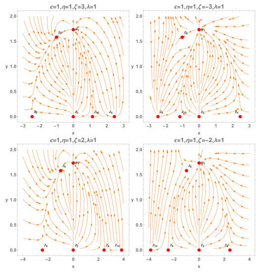
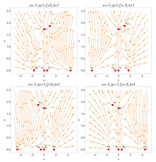
Phase-space diagrams for the dynamical system (21) and (22) where the scalar field is a quintessence are presented in Figure 1.
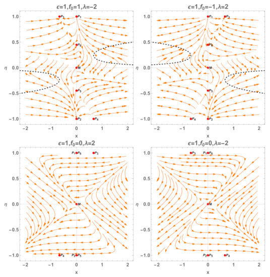
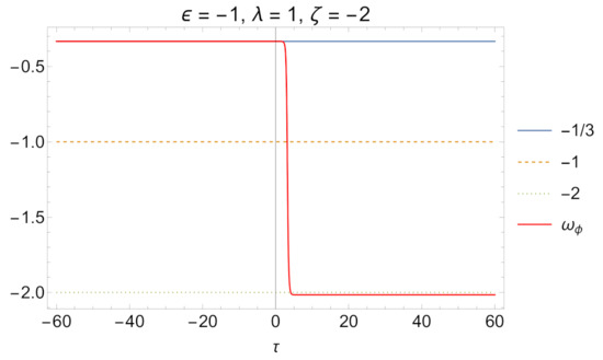
Figure 2 depicts , , and evaluated at the solution of system (21) and (22) for and initial conditions (i.e., near the saddle point ).
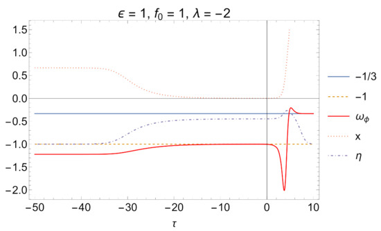
Figure 2.
, and evaluated at the solution of system (21) and (22) for and initial conditions (i.e., near the saddle point ). The solution is past asymptotic to a phantom regime , then remains near the de Sitter point approaching the phantom solution (whence ), then crosses from below of (zero acceleration), decelerating and tending asymptotically to from above.
The solution is past asymptotic phantom regime , and then remains near the de Sitter point approaching the phantom solution (whence ), then crosses from below of (zero acceleration), decelerating and tending asymptotically to from above. This evolution, in which the equation of state parameter of the scalar field interpolates between (saddle point, de Sitter solution) and (attractor dominated by the Gauss–Bonnet term), corresponds to an inflationary solution, which does not eliminate the topological defect of the cosmic string. This behavior is due to the linear coupling between the scalar field and the Gauss–Bonnet term.
3.2. Dynamical System Analysis of 2D System for
In this section, we perform the stability analysis for the equilibrium points of system (21) and (22), taking .
The stability results and physical observable results for system (21) and (22) are summarized in Table 2.
The equilibrium points in the coordinates are the following.
- , with eigenvalues . The asymptotic solution corresponds to the Minkowski spacetime.
- , with eigenvalues The deceleration parameter is . That means the asymptotic solution describes a universe dominated by the Gauss–Bonnet term. This equilibrium point is a source.
- , with eigenvalues with . This equilibrium point is a sink. The asymptotic solution is similar to that of point .
- , with eigenvalues This equilibrium point is a sink. Moreover, means that the asymptotic behavior is similar to that of
- , with eigenvalues , while the deceleration parameter is calculated . This equilibrium point is a source. As before, the asymptotic solution is similar to point .
- , with eigenvalues . This equilibrium point corresponds to a de Sitter solution, i.e., . This equilibrium point exists for , or and is a saddle.
- with eigenvalues , is a de Sitter point that is . This equilibrium point exists for or , and is a saddle.
- This equilibrium point exists for , has eigenvalues and is a sink for , a saddle for or nonhyperbolic for Moreover, is from where we infer that the asymptotic solution is that of the de Sitter universe. The numerical analysis of the real part of the eigenvalues for is presented in Figure 3.
- describes a de Sitter solution because . This equilibrium point exists for , has eigenvalues , and is a source for , a saddle for or nonhyperbolic for As before, the numerical analysis of the real part of the eigenvalues for is presented in Figure 3.
- This equilibrium point exists for , it describes a de Sitter solution because , has eigenvalues and is a source for , a saddle for or nonhyperbolic for The numerical analysis of the real part of and for is presented in Figure 3.
- Finally, the de Sitter point This equilibrium point exists for , has eigenvalues and is a sink for , a saddle for or nonhyperbolic for As before, the numerical analysis of the real part of and for is presented in Figure 3.


Figure 3.
Real part of the eigenvalues where for points .
Figure 3.
Real part of the eigenvalues where for points .


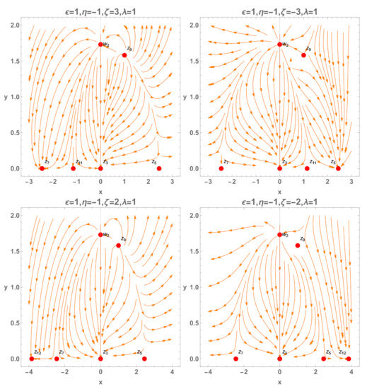
Phase-space diagrams for the dynamical system (21) and (22) where the scalar field is a phantom field, that is, are presented in Figure 4 for various values of the free parameters.
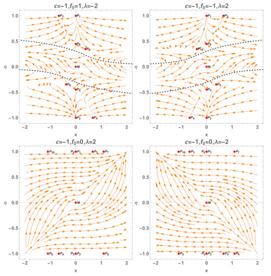
Figure 5 depicts , , and evaluated at the solution of system (21) and (22) for and initial conditions (i.e., near the saddle point ).
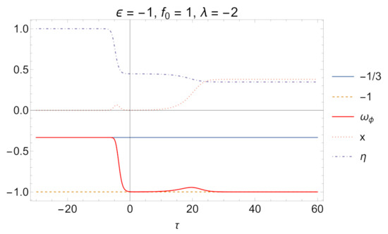
Figure 5.
, , and evaluated at the solution of system (21) and (22) for and initial conditions (i.e., near the saddle point ). The solution is past asymptotic to (zero acceleration), then remains near the de Sitter point approaching a quintessence solution , and then, tending asymptotically to (de Sitter point ) from above.
The solution is past asymptotic to (zero acceleration), then remains near the de Sitter point approaching a quintessence solution , and then tending asymptotically to (de Sitter point ) from above. The past attractor is dominated by the Gauss–Bonnet term, and then the saddle point corresponds to an inflationary solution, eliminating the topological defect of the cosmic string. The late-time attractor is a de Sitter solution. Therefore, this solution connects inflation with late-time acceleration. This behavior is due to the linear coupling between the scalar field and the Gauss–Bonnet term.
3.3. Analysis of System (21) and (22) at Infinity
The numerical results in Figure 1 and Figure 4 suggest non-trivial dynamics when . For that reason, we introduce the compactified variable
and the new time variable
we obtain the compactified dynamical system
where The limit corresponds to .
The equilibrium points of system (27) and (28) at the finite region are the same as (21) and (22) by the rescaling .
Table 3 summarizes the equilibrium points of system (27) and (28) for with their stability conditions.
The equilibrium points at infinity are those satisfying , say
- , with eigenvalues This equilibrium point is a saddle or nonhyperbolic for The value of the deceleration parameter is . That means the asymptotic solution describes a universe dominated by the Gauss–Bonnet term.
- , with eigenvalues This equilibrium point is a saddle or nonhyperbolic for The value of the deceleration parameter is The asymptotic behavior is the same as
- , with eigenvalues This equilibrium point is a saddle or nonhyperbolic for The value of the deceleration parameter is The asymptotic behavior is the same as
- , with eigenvalues This equilibrium point is a saddle or nonhyperbolic for The value of the deceleration parameter is The asymptotic behavior is the same as
- , with eigenvalues . This equilibrium point is a source for , a sink for or nonhyperbolic for Note that for
- (a)
- , the equilibrium point has This equilibrium point exists for or or
- (b)
- , the equilibrium point has This equilibrium point exists for or or
The value of the deceleration parameter is The asymptotic solution is a de Sitter universe. - , with eigenvalues . This equilibrium point is a sink for , a source for or nonhyperbolic for The existence conditions for are the same as The value of the deceleration parameter is The asymptotic behavior is the same as
- , with eigenvalues . This equilibrium point is a source for , a sink for ; or nonhyperbolic for The existence conditions for are the same as The value of the deceleration parameter is The asymptotic behavior is the same as
- , with eigenvalues . This equilibrium point is a sink for , a source for or nonhyperbolic for The existence conditions for are the same as The value of the deceleration parameter is The asymptotic behavior is the same as
The phase-space of the field equations at the new compactified variables is presented in Figure 6 and Figure 7 for different values of the free parameters. As far as the physical properties of the asymptotic solutions are concerned, we find that , , , and are Gauss–Bonnet points with deceleration parameter , while points , , , and are de Sitter points with .
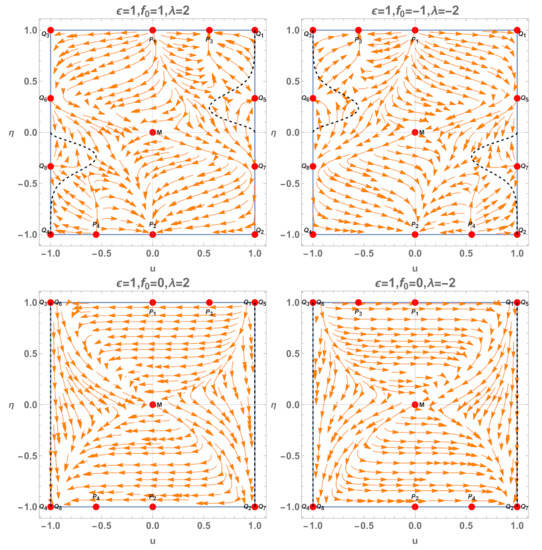
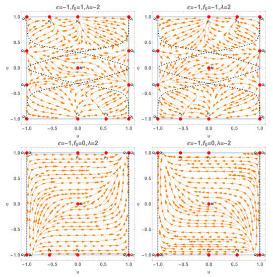
Figure 8 depicts , , and evaluated at the solution of system (27) and (28) for initial conditions (i.e., near the saddle point ).
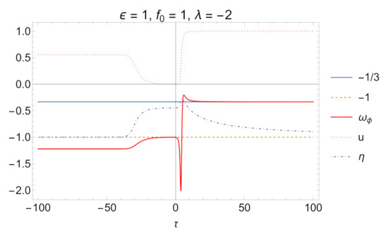
Figure 8.
, , and evaluated at the solution of system (27) and (28) for initial conditions (i.e., near the saddle point ). The solution is past asymptotic to a phantom regime , then remains near the de Sitter point approaching the phantom solution (whence ), and then crosses from below (zero acceleration), decelerating and tending asymptotically to from above.
The solution is past asymptotic to a phantom regime , then remains near the de Sitter point approaching the phantom solution (whence ), then it crosses from below (zero acceleration), decelerating and tending asymptotically to from above. As before, this evolution corresponds to an inflationary solution, which does not eliminate the topological defect of the cosmic string. This behavior is due to the linear coupling between the scalar field and the Gauss–Bonnet term.
Figure 9 depicts , , and evaluated at the solution of system (27) and (28) for and initial conditions (i.e., near the saddle point ).
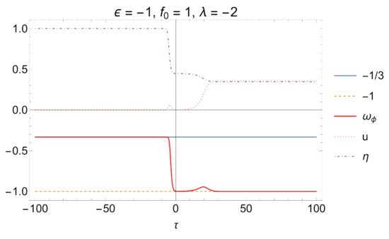
Figure 9.
, , and evaluated at the solution of system (27) and (28) for and initial conditions (i.e., near the saddle point ). The solution is past asymptotic to (zero acceleration), then remains near the de Sitter point approaching a quintessence solution , then tending asymptotically to (de Sitter point ) from above.
The solution is past asymptotic to (zero acceleration), then remains near the de Sitter point approaching a quintessence solution , and then tending asymptotically to (de Sitter point ) from above. The past attractor is dominated by the Gauss–Bonnet term, and then the saddle point corresponds to an inflationary solution, eliminating the topological defect of the cosmic string. The late-time attractor is a de Sitter solution. Therefore, this solution connects inflation with late-time acceleration. This behavior is due to the linear coupling between the scalar field and the Gauss–Bonnet term.
4. Phase-Space Analysis for Exponential :
The field equations for the exponential coupling are given by the following expressions:
where the dot means derivative with respect to t, and the comma means derivative with respect to the function’s argument.
Defining the normalized variables
we can write the Friedmann equation as
In addition, the deceleration and EoS parameters are given by
and
4.1. Dynamical System Analysis of 3D System for
Table 4 summarizes the equilibrium points of this system with their stability conditions. It also includes the value of and
- , with eigenvalues This set of equilibrium points exists for and is nonhyperbolic. The asymptotic solution at the equilibrium point describes the Minkowski spacetime.
- , with eigenvalues This equilibrium point is a source. For the deceleration parameter, we derive . The asymptotic solution describes a universe dominated by the Gauss–Bonnet term.
- , with eigenvalues This equilibrium point is a sink. Since , the physical properties are similar to point
- with eigenvalues Moreover, means that the asymptotic solution describes a stiff fluid solution. This equilibrium point is a
- (a)
- source for , ;
- (b)
- saddle for or ;
- (c)
- nonhyperbolic for or
- , with eigenvalues and , represents a stiff fluid solution. This equilibrium point is a
- (a)
- sink for , ;
- (b)
- saddle for or ;
- (c)
- nonhyperbolic for or
- , with eigenvalues and , represents a stiff fluid solution. This equilibrium point is a
- (a)
- source for , ;
- (b)
- saddle for or ;
- (c)
- nonhyperbolic for or
- , with eigenvalues and , represents a stiff fluid solution. This equilibrium point is
- (a)
- sink for , ;
- (b)
- saddle for or ;
- (c)
- nonhyperbolic for or
- , with eigenvalues . This equilibrium point exists for and is
- (a)
- a saddle for
- i.
- or
- ii.
- or
- iii.
- or
- iv.
- and
- (b)
- nonhyperbolic for
- i.
- or
- ii.
- or
- iii.
- or
- iv.
As before, we calculate from where we infer that acceleration occurs for . - , with eigenvalues . This equilibrium point exists for and is
- (a)
- a saddle for
- i.
- or
- ii.
- or
- iii.
- or
- iv.
- and
- (b)
- nonhyperbolic for
- i.
- or
- ii.
- or
- iii.
- or
- iv.
Furthermore, for the asymptotic solution at the equilibrium point, we derive from where we infer that acceleration occurs for . - , wherewhere This equilibrium point exists for but For , we haveThe eigenvalues of are for Given the complexity of the expressions, we perform numerical analysis to conclude that this equilibrium point is a source or saddle (see Figure 10).
 Figure 10. Real part of the eigenvalues of for and . The equilibrium point has a source or saddle behavior.The physical parameters and are presented in Figure 11.Figure 10. Real part of the eigenvalues of for and . The equilibrium point has a source or saddle behavior.
 Figure 11. Plot of and . We see that if , then and .The equilibrium points can describe dust-like and radiation-like cosmological eras; however, , the solution, cannot describe an accelerated universe. For large and small values of we have that and .Figure 11. Plot of and . We see that if , then and .
- , wherewhere This equilibrium point exists for and For this equilibrium point, we haveThe eigenvalues of are for Given the complexity of the expressions, we perform numerical analysis to conclude that this equilibrium point is a saddle (see Figure 12).
 Figure 12. Real part of the eigenvalues of . This equilibrium point is a saddle.We have presented plots for the case because the other interval produces similar (symmetric) results. In Figure 13, we give the evolution of the physical parameters and in terms of the free parameter .Figure 12. Real part of the eigenvalues of . This equilibrium point is a saddle.
 Figure 13. Plot of and . For large we have that and .Thus, the asymptotic solution describes ideal gas solutions, but an accelerated universe cannot be described. However, dust-like and radiation-like epochs are provided by the equilibrium points. For large , we have that and .Figure 13. Plot of and . For large we have that and .
- , wherewhere This equilibrium point exists for The eigenvalues for are ; given the complexity of the expressions, we perform numerical analysis to conclude that this equilibrium point is a sink or saddle (see Figure 14).
 Figure 14. Real part of the eigenvalues of . This equilibrium point has sink or saddle behavior.For , we have and ; given that these are long expressions, we write them as , but we verify that for , and , see Figure 15.Figure 14. Real part of the eigenvalues of . This equilibrium point has sink or saddle behavior.

Figure 15.
Plot of and . We verify that , and .
Figure 15.
Plot of and . We verify that , and .

Phase-space diagrams for a 2D projection setting , and different values of are presented in Figure 16. We also present similar diagrams for the other 2D projection setting in Figure 17. The existence of the equilibrium points , and is discussed in Appendix A.
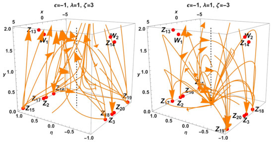
Three-dimensional phase-space diagrams are presented in Figure 18 setting , and different values of Figure 18 depicts a three–dimensional phase plot of of system (35)–(37) setting with different values of . Here, the saddle points and are singularities in which both the numerator and denominator of the y equation vanish.
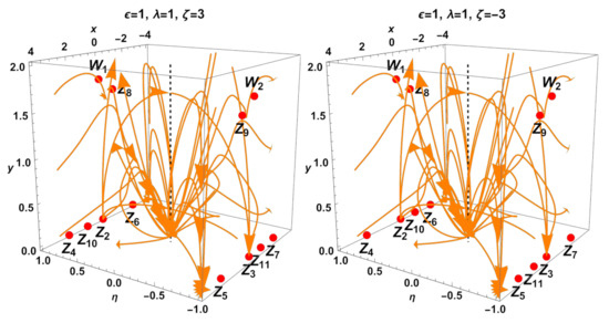
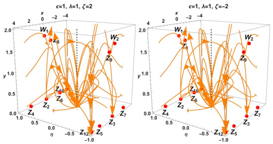

Figure 19.
evaluated at the solution of system (35)–(37) for and initial conditions . The solution is past asymptotic to (zero acceleration, cosmic string fluid), then crosses the line (superluminal evolution) twice, remaining near the de Sitter point (de Sitter point, inflation) from above, following an era where (domain wall), before an accelerated de Sitter solution (late-time acceleration).
The solution is past asymptotic to (zero acceleration, cosmic string fluid), then crosses the line (superluminal evolution) twice, remaining near the de Sitter point (de Sitter point, inflation) from above, following an era where (domain wall), before an accelerated de Sitter solution (late-time acceleration). The the past attractor is dominated by the Gauss–Bonnet term. Then, the saddle point corresponds to an inflationary solution with , eliminating the topological defect of the cosmic string. At the latter stage, the solution has corresponding to a domain wall. The late-time attractor is a de Sitter solution that allows the latter cosmological defect to exit. Therefore, this solution connects inflation with late-time acceleration. This behavior is due to the exponential coupling between the scalar field and the Gauss–Bonnet term.
4.2. Dynamical System Analysis of 3D System for
Table 5 summarizes the equilibrium points of this system with their stability conditions. It also includes the value of and
- , with eigenvalues This is a nonhyperbolic set of points for . The asymptotic solution at the equilibrium point describes the Minkowski spacetime.
- , with eigenvalues This equilibrium point is a source and we verify that . The asymptotic solution describes a universe dominated by the Gauss–Bonnet term.
- , with eigenvalues This equilibrium point is a sink, and we also have that . The asymptotic behavior is similar to that of
- , with eigenvalues For this equilibrium point, we have ; this means that acceleration occurs for . The equilibrium points are
- (a)
- sinks for
- i.
- and or
- ii.
- and and
- (b)
- saddle for
- i.
- and or
- ii.
- and
- (c)
- nonhyperbolic for or
- , with eigenvalues For this equilibrium point, we have ; this means that acceleration occurs for . The equilibrium points are
- (a)
- sources for
- i.
- and or
- ii.
- and and
- (b)
- saddle for
- i.
- and or
- ii.
- and
- (c)
- nonhyperbolic for or
- , where andThis equilibrium point exists for but We verify thatThe eigenvalues for are , with . Given the complexity of these expressions, we perform the analysis numerically and present it in Figure 20.We conclude that the equilibrium point has a source or saddle behavior. In Figure 21, we show that and are always positive and they go to infinity as .
- , where andThis equilibrium point exists for but For , we have and . The eigenvalues for are , with ; given the complexity of the expressions, we perform numerical analysis to conclude that this equilibrium point is a sink or saddle, see Figure 22. Since the expressions for the EoS and deceleration parameters are lengthy and complicated, we write them as . However, we verify that they are both negative and for , we have that and see , see Figure 23.
- , where and
- , where and.
- , where andThis equilibrium point exists for but The eigenvalues are for The stability analysis is performed numerically in Figure 28 where we see that has sink or saddle behavior. For , we have that , and that is, are complicated expressions that depend on and ; therefore, we study them in Figure 29 and see that they are always positive and go to ∞ as
- , where andThis equilibrium point exists for but The eigenvalues of are for . Figure 30 represents the real part of the eigenvalues of ; we see that the equilibrium point has saddle behavior.For the EoS and deceleration parameters, they can be written as , and we verify that they are both negative. In Figure 31 are presented plots of and ; we see that they are both negative but and

Figure 20.
Real part of the eigenvalues of This equilibrium point is a source or a saddle.
Figure 20.
Real part of the eigenvalues of This equilibrium point is a source or a saddle.


Figure 21.
Plot of and ; they are both positive and go to as .
Figure 21.
Plot of and ; they are both positive and go to as .


Figure 22.
Real part of the eigenvalues of This equilibrium point has sink or saddle behavior.
Figure 22.
Real part of the eigenvalues of This equilibrium point has sink or saddle behavior.


Figure 23.
Plot of and ; they are both negative and go to as .
Figure 23.
Plot of and ; they are both negative and go to as .


Figure 24.
Real part of the eigenvalues of ; we see that the equilibrium point has saddle behavior.
Figure 24.
Real part of the eigenvalues of ; we see that the equilibrium point has saddle behavior.


Figure 25.
Plot of and Here we see that and as .
Figure 25.
Plot of and Here we see that and as .


Figure 26.
Real part of the eigenvalues of ; we can see that the equilibrium point is a source.
Figure 26.
Real part of the eigenvalues of ; we can see that the equilibrium point is a source.


Figure 27.
Plot of and ; we see that both are negative and go to as .
Figure 27.
Plot of and ; we see that both are negative and go to as .


Figure 28.
Real part of the eigenvalues of ; we see that the equilibrium point has sink or saddle behavior.
Figure 28.
Real part of the eigenvalues of ; we see that the equilibrium point has sink or saddle behavior.


Figure 29.
Plots for and ; we see that both are positive and go to ∞ as .
Figure 29.
Plots for and ; we see that both are positive and go to ∞ as .


Figure 30.
Real part of the eigenvalues of ; we see that the equilibrium point has saddle behavior.
Figure 30.
Real part of the eigenvalues of ; we see that the equilibrium point has saddle behavior.


Figure 31.
Plots of and ; we see that they are both negative but and .
Figure 31.
Plots of and ; we see that they are both negative but and .

In Figure 32, we present phase-space diagrams for a 2D projection of system (35)–(37) setting , and different values of Also three dimensional phase-space diagrams are presented in Figure 33 for and different values of The results of this section are summarized in Table 5. The existence of the equilibrium points is discussed in Appendix A.
The solution is past asymptotic to and future asymptotic to a phantom solution with (late-time acceleration). The late-time attractor is a phantom solution that allows the latter cosmological defect to exit. This behavior is due to the exponential coupling between the scalar field and the Gauss–Bonnet term.
4.3. Analysis of System (35)–(37) at Infinity: Poincaré Variables
The numerical results presented in Figure 18 and Figure 33 suggest that there are non-trivial dynamics when and . For that reason, we introduce the Poincaré compactification variables along with the definition of
We must find evolution equations for . Note that the limit corresponds to .
Using the Equations (35)–(37) and the variables (49), we obtain the following system
defined on the phase-space
Here, we used the notation
and defined a new time variable by
4.3.1. Analysis of System (50)–(52) for
This section presents the analysis of system (50)–(52) for the quintessence field (). The equilibrium points of the system, with their stability conditions, are summarized in Table 6.
- with eigenvalues This is a nonhyperbolic set of point with and
- with eigenvalues For this equilibrium point, we have that and blow up for , so we present the analysis in Figure 35. We see that for and negative values of , and tend to minus infinity as but they tend to and 0, respectively, as For positive values of and , the opposite occurs, and tend to infinity as , but they tend to and 0, respectively, as If we consider negative values of and , the behavior is symmetric. We also see that this equilibrium point is
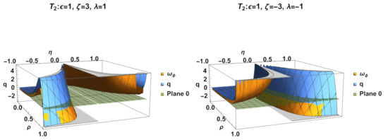 Figure 35. Plots of for . We see that for and negative values of , the physical observables tend to minus infinity as ; for positive values of and , the opposite occurs, and tend to infinity as .
- (a)
- a saddle for , ,
- (b)
- nonhyperbolic for
- i.
- or
- ii.
- .
- , with eigenvalues For this equilibrium point, the behavior of and is similar that for , meaning that these parameters blow up as goes to 0. Taking a sign change in in Figure 35 we show a symmetric behavior in Figure 36. This equilibrium point is also
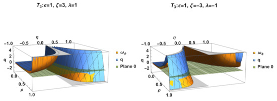 Figure 36. Plots of and q for . We see that for and negative values of , the physical observables tend to infinity as ; for positive values of and , the opposite occurs, and tend to minus infinity as .
- (a)
- a saddle for , ,
- (b)
- nonhyperbolic for
- i.
- or
- ii.
- .
- with eigenvalues For these equilibrium points, we have and We verify that and are directed infinity that depend on the sign of However, for , we have that and , see Figure 37. Performing the stability analysis, we see that the equilibrium points are
 Figure 37. Plots of for We see that and are directed infinity depending on the sign of .
- (a)
- saddle for , ,
- (b)
- nonhyperbolic for
- i.
- or
- ii.
- .
- with eigenvalues . For these equilibrium points, we have and We verify that and are directed infinity that depend on the sign of However, for , we have that and , see Figure 38. By performing the stability analysis, we conclude that the equilibrium points are
 Figure 38. Plots of for We see that and are directed infinity depending on the sign of .
- (a)
- saddle for , ,
- (b)
- nonhyperbolic for
- i.
- or
- ii.
- .
- , with eigenvalues This equilibrium point is a saddle and has and
- , with eigenvalues This equilibrium point is a saddle and has and
- , with eigenvalues This equilibrium point is a source and has and
- , with eigenvalues This equilibrium point is a sink and has and
- , with eigenvalues This equilibrium point is a saddle and has and
- , with eigenvalues This equilibrium point is a saddle and has and
- with eigenvalues is represented in Figure 39 as a dashed red line. This set of points is nonhyperbolic with and
The equilibrium points with have ; this means that in the finite case, Additionally, since , the asymptotic solution for these points represents a universe dominated by the Gauss–Bonnet term.
4.3.2. Analysis of System (50)–(52) for
This section presents the analysis of system (50)–(52) for the phantom field (). The equilibrium points of the system, with their stability conditions, are summarized in Table 7.
- , with eigenvalues this set of points is nonhyperbolic. For this equilibrium point, we have and
- with eigenvalues . The stability analysis is performed similarly to Section 4.3.1. For the study of and , we see that these expressions blow up for ; because of this, we present Figure 40. For , we verify that and . On the other direction, that is , we have and .
- , with eigenvalues The stability analysis is the same as in Section 4.3.1. Since the EoS and deceleration parameters blow up for , we study their behavior in Figure 41. For , we verify that and . On the other direction, that is , we have and .
- , with eigenvalues The stability analysis is the same as in Section 4.3.1. However, we verify that the limit as of the EoS and deceleration parameters are directed infinity that depend on the sign of We also see that and , see Figure 42.
- , with eigenvalues The stability analysis is the same as in Section 4.3.1. Something similar (to the previous two points) occurs to and ; that is, they have directed infinity, but in this case, they depend on the sign of , see Figure 43.
- , with eigenvalues This equilibrium point is a saddle and has and
- , with eigenvalues This equilibrium point is a saddle and has and
- , with eigenvalues This equilibrium point is a source and has and
- , with eigenvalues This equilibrium point is a sink and has and
- , with eigenvalues This equilibrium point is a saddle and has and
- , with eigenvalues This equilibrium point is a saddle and has and
- with eigenvalues . This set of points is nonhyperbolic with and

Figure 40.
Plots of and q for . The values of the physical observables are directed infinity that depend on the sign of and the direction from which we approach .
Figure 40.
Plots of and q for . The values of the physical observables are directed infinity that depend on the sign of and the direction from which we approach .


Figure 41.
Plot of and q for The values of the physical observables are directed infinity that depend on the sign of and the direction from which we approach .
Figure 41.
Plot of and q for The values of the physical observables are directed infinity that depend on the sign of and the direction from which we approach .


Figure 42.
Plot of for We see that and are directed infinity depending on the sign of .
Figure 42.
Plot of for We see that and are directed infinity depending on the sign of .


Figure 43.
Plot of for We see that and are directed infinity depending on the sign of .
Figure 43.
Plot of for We see that and are directed infinity depending on the sign of .

Recall that the equilibrium point s with have ; this means that in the finite case, Additionally, since , the asymptotic solution for these points represents a universe dominated by the Gauss–Bonnet term. We also have the following additional points where For these remaining points, we perform numerical analysis both on the real part of the eigenvalues and the behavior of and
- The eigenvalues are for ; the analysis is performed for some values of and in Figure 44, where we see that the equilibrium point has a saddle or sink behavior. However, since , the equilibrium point has source behavior in the limit . For this equilibrium point, we verify that both and go to infinity as ; therefore, the equilibrium point cannot describe an accelerated universe regardless of the values of , and , see Figure 45. We also verify that they tend to and 0, respectively, as
- The eigenvalues are for ; the analysis is performed for some values of and in Figure 46. The equilibrium point has saddle or source behavior. The equilibrium point has sink behavior as . In addition, we verify that both and go to infinity as . That means that the equilibrium point cannot describe an accelerated universe regardless of the values of and , see Figure 47; we also verify that and tends to and 0, respectively, as
- The eigenvalues are with The equilibrium point has saddle behavior for values of ; however, since is zero for this equilibrium point, is nonhyperbolic, see Figure 52. The physical parameters and blow up for , see Figure 53. In particular, we verify that and ; given this, the equilibrium point cannot describe an accelerated universe.
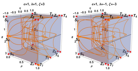
In Figure 56, we present some three-dimensional phase-plot diagrams for , , and different values of .

Figure 44.
Real part of the eigenvalues of for different values of the parameters and with These equilibrium points exhibits source behavior for .
Figure 44.
Real part of the eigenvalues of for different values of the parameters and with These equilibrium points exhibits source behavior for .


Figure 45.
Plots of for They go to infinity as .
Figure 45.
Plots of for They go to infinity as .


Figure 46.
Real part of the eigenvalues of for different values of the parameters and with This equilibrium points exhibits saddle, source, or sink behavior.
Figure 46.
Real part of the eigenvalues of for different values of the parameters and with This equilibrium points exhibits saddle, source, or sink behavior.


Figure 47.
Plots of for They go to infinity as .
Figure 47.
Plots of for They go to infinity as .


Figure 48.
Real part of the eigenvalues of for different values of the parameters and with This equilibrium point exhibits source behavior as .
Figure 48.
Real part of the eigenvalues of for different values of the parameters and with This equilibrium point exhibits source behavior as .


Figure 49.
Plots of for They go to infinity as .
Figure 49.
Plots of for They go to infinity as .


Figure 50.
Real part of the eigenvalues of for different values of the parameters and with This equilibrium point exhibits saddle, source, or sink behavior.
Figure 50.
Real part of the eigenvalues of for different values of the parameters and with This equilibrium point exhibits saddle, source, or sink behavior.


Figure 51.
Plots of for They go to infinity as .
Figure 51.
Plots of for They go to infinity as .


Figure 52.
Real part of the eigenvalues of for different values of the parameters and with and This equilibrium point exhibits saddle or nonhyperbolic behavior.
Figure 52.
Real part of the eigenvalues of for different values of the parameters and with and This equilibrium point exhibits saddle or nonhyperbolic behavior.


Figure 53.
Plots of for They go to infinity as .
Figure 53.
Plots of for They go to infinity as .


Figure 54.
Real part of the eigenvalues of for different values of the parameters and with and This equilibrium point exhibits saddle and nonhyperbolic behavior.
Figure 54.
Real part of the eigenvalues of for different values of the parameters and with and This equilibrium point exhibits saddle and nonhyperbolic behavior.


Figure 55.
Plots of for They go to infinity as .
Figure 55.
Plots of for They go to infinity as .


5. Conclusions
In this work, we considered a four-dimensional FLRW geometry and a second-order modified gravitational theory with a scalar field coupled to the Gauss–Bonnet scalar. The Gauss–Bonnet term does not contribute to the gravitational Action Integral in the limit where the scalar field is constant. The theory reduces to General Relativity with a cosmological constant term. However, for a dynamical scalar field, the physical properties of the present cosmological model are distinct from that of the minimally coupled scalar field theory.
In order to study the dynamical properties of the phase-space and physical variables, we introduced dimensionless variables different from that of the H-normalization. The latter is because, from the field equations, we observed that it is possible in Einstein–Gauss–Bonnet scalar field theory that the Hubble function can change its sign during its evolution, which means it can vanish. Hence, the H-normalization, widely applied before, must be validated for global analysis and the complete reconstruction of the cosmological history and epochs. Additionally, we observed that the dynamical variables are not bounded in a finite regime, which means that to perform a complete study of the phase-space, we assumed compactified variables to investigate the asymptotic behavior of the model at infinity.
The phase-space analysis of the gravitational field equations is a novel mathematical approach to the model’s asymptotic description and evolution of the physical variables. In cosmological studies, such analysis provides essential information about the significant cosmological eras the theory provides. Simultaneously, important conclusions about the viability of the theory can be made. According to cosmological observations, some particular forms of matter at each stage seem to dominate evolution. The required dominance should be translated into different critical points, around which cosmological solutions remain a lapse of time before approaching a stable late-time configuration. In the dynamical systems language, complete cosmological dynamics [75] can be understood as an orbit connecting a past attractor, also called a source, with a late-time attractor, called a sink, that passes through some saddle points such that radiation precedes matter domination. These are often the extreme points of the orbits and therefore describe the asymptotic behavior. However, some solutions interpolate between critical points and then provide information on the intermediate stages of the evolution, with interest in orbits corresponding to a specific cosmological history [76,77,78,79]. However, according to our setup, we have partial cosmological dynamics. Therefore, the analysis incorporating additional matter fields to complete cosmological dynamics is left to a forthcoming investigation.
The gravitational Action Integral depends on two functions, which are the coupling function of the scalar field with the Gauss–Bonnet scalar and the scalar field potential. For the coupling functions, we consider two functional forms, the exponential function, a power-law function, while the potential we assume to be the exponential functional form. Moreover, a parameter has been introduced in the kinetic part of the scalar field, such that the scalar field is a quintessence field, , or a phantom field, . The two functional forms for the coupling function of the scalar field with the Gauss–Bonnet scalar provide different cosmological evolution. Last, but not least, the stability properties of the asymptotic solutions were investigated.
For the linear coupling function with a quintessence scalar field, we have found the following equilibrium points for the system (21) and (22) for , as it was summarized in Table 1. Say,
- , which does not appears in the reference [72], because it corresponds to . It is nonhyperbolic, and the effective EoS and deceleration parameters are indeterminate.
- The sources points are and , which have , and which are related to cosmic strings.
- The sinks are and , which have , and , therefore, they are related to cosmic strings.
- The de Sitter solutions ( and ), are saddle.
To present one possible evolution of the physical model, Figure 2 depicts , and evaluated at the solution of system (21) and (22) for for initial conditions near the saddle point . The solution is past asymptotic to a phantom regime , then remains near the de Sitter point approaching the phantom solution (whence ), and then crosses from below (zero acceleration), decelerating and tending asymptotically to from above. This evolution, in which the equation of state parameter of the scalar field interpolates between and , corresponds to an inflationary solution, which does not eliminate the topological defect of the cosmic string. This behavior is due to the linear coupling between the scalar field and the Gauss–Bonnet term.
For the linear coupling function with a phantom scalar field, we have found the following equilibrium points for the system (21) and (22) for , as it was summarized in Table 2.
- As for the quintessence field, the stability conditions and the physical interpretation of (with and q indeterminate), and (which have , and ) which are related to cosmic strings, and the Sitter solutions ( and ) are the same as for quintessence.
- Because of the phantom’s negative kinetic energy, we obtain new points compared with the quintessence case. For example is sink for , a saddle for , or nonhyperbolic for .
- Moreover, is a source for , a saddle for , or nonhyperbolic for .
- Furthermore, the equilibrium point is source for , a saddle for , or nonhyperbolic for .
- Finally, is a sink for , a saddle for , or nonhyperbolic for . The four solutions are de Sitter solutions with and which can be late-time, early-time solutions, or intermediate stages in the evolution.
To present one possible evolution of the physical model, Figure 5 depicts , , and evaluated at the solution of system (21) and (22) for and initial conditions near the saddle point . The solution is past asymptotic to , then remains near the de Sitter point approaching a quintessence solution , and then tending asymptotically to (de Sitter point ) from above. The past attractor is dominated by the Gauss–Bonnet term, and then the saddle point corresponds to an inflationary solution, eliminating the topological defect of the cosmic string. The late-time attractor is a de Sitter solution. Therefore, this solution connects inflation with late-time acceleration. This behavior is due to the linear coupling between the scalar field and the Gauss–Bonnet term.
Because there is non trivial dynamics as , we have introduced a compactified variable . The equilibrium points of system (27) and (28) at the finite region are the same as of (21) and (22) by the re-scaling accordingly; whereas, the equilibrium points at infinity, which are those satisfying , are summarized in Table 3. They are the following.
- and are saddle for , nonhyperbolic for . They corresponds to cosmic strings with , .
- The de Sitter solutions with infinity x are , which are sink for , source for , or nonhyperbolic for , and , which are source for , sink for , nonhyperbolic for .
As per the evolution of the observables regards, we have produced Figure 8 and Figure 9, which retain the information of Figure 2 and Figure 5, respectively, as .
For the exponential coupling function with a quintessence scalar field, we have found the following equilibrium points in the coordinates of system (35)–(37) for . Say, we obtain the following equilibrium points at the finite region. The stability analysis of the equilibrium point of the system is summarized in Table 4.
- The line of equilibrium points that is nonhyperbolic with and q indeterminate.
- The equilibrium point is a source with and .
- The equilibrium point is sink and .
- The equilibrium point is source for , a saddle for or , or nonhyperbolic for or . The cosmological observables are , . It is a stiff-matter solution.
- The equilibrium point is sink for , a saddle for or , or nonhyperbolic for or . The cosmological observables are , . It is a stiff-matter solution.
- The equilibrium point . It is a source for , a saddle for or , or nonhyperbolic for or . The cosmological observables are , . It is a stiff-matter solution.
- The equilibrium point . It is a sink for , a saddle for or , or nonhyperbolic for or .
- The equilibrium point is nonhyperbolic for , or a saddle for , or , or , or .
- The equilibrium point is nonhyperbolic for , or a saddle for , or , or , or . For , the cosmological observables are and , from where we infer that acceleration occurs for .
To present one possible evolution of the physical model, Figure 19 depicts evaluated at the solution of system (35)–(37) for and initial conditions . The solution is past asymptotic to (zero acceleration, cosmic string fluid), then crosses the line (superluminal evolution) twice, remaining near the de Sitter point (de Sitter point, inflation) from above, following an era where (domain wall), before an accelerated de Sitter solution (late-time acceleration). The past attractor is dominated by the Gauss–Bonnet term. Then, the saddle point corresponds to an inflationary solution with , eliminating the topological defect of the cosmic string. At the latter stage, the solution has corresponding to a domain wall. The late-time attractor is a de Sitter solution that allows the latter cosmological defect to exit. Therefore, this solution connects inflation with late-time acceleration. This behavior is due to the exponential coupling between the scalar field and the Gauss–Bonnet term.
For the exponential coupling function with a phantom scalar field, we have found the following equilibrium points of system (35)–(37) for summarized in Table 5. They are the following.
- The line of equilibrium points is nonhyperbolic with EoS and deceleration parameters indeterminate.
- The equilibrium point is a source with and , and is a sink with and . They have the same behavior as the analogous point in the quintessence case.
- Because of the phantom’s negative kinetic energy, we obtain new points compared with the quintessence case. For example is nonhyperbolic for or , or a sink for , or , or a saddle for , or .
- The equilibrium point is nonhyperbolic for or , a source for , or . It is a saddle for , or . The cosmological observables for are and ; they are always phantom accelerated solutions.
To present one possible evolution of the physical model, Figure 34 depicts evaluated at the solution of system (35)–(37) for and initial conditions . The solution is past asymptotic to and future asymptotic to a phantom solution with (late-time acceleration). The late-time attractor is a phantom solution that allows the latter cosmological defect to exit. This behavior is due to the exponential coupling between the scalar field and the Gauss–Bonnet term.
Because there are non-trivial dynamics at infinity, we have introduced the Poincaré compactification variables along with the definition of as given by (49) which leads to the system (50)–(52). The equilibrium points are the following.
- . It is nonhyperbolic. The cosmological observables are , and .
- The equilibrium point is a saddle. The EoS parameter and the deceleration parameter are represented in Figure 35.
- The equilibrium point is a saddle. The EoS parameter and the deceleration parameter are represented in Figure 36.
- The equilibrium point is a saddle. The EoS parameter and the deceleration parameter are represented in Figure 37.
- The equilibrium point is a saddle. The EoS parameter and the deceleration parameter are represented in Figure 38.
- The equilibrium point is a saddle.
- The equilibrium point is a saddle.
- The equilibrium point is a source.
- The equilibrium point is a sink.
- The equilibrium point is a saddle.
- The equilibrium point is a saddle.
- The equilibrium point is nonhyperbolic. The cosmological observables of to are and . They correspond to cosmic string solutions.
- As in the quintessence case, the equilibrium points from to and to are the same. Their stability conditions and cosmological interpretations are identical to the analogous quintessence points.
- Because of the phantom’s negative kinetic energy, we obtain new points compared with the quintessence case. For example , where , , , , , . By analyzing numerically and q, we conclude that to cannot correspond to the current accelerated universe since and as .
This study extends and completes previous results in the literature in Einstein–Gauss–Bonnet scalar field cosmology [71,72]. The analysis indicates that the theory can explain the main eras of cosmological history. We plan to extend the further analysis in future work by introducing matter source components and new functional forms for the scalar field potential and the coupling function.
Author Contributions
Conceptualization, A.D.M. and A.P.; methodology, A.D.M. and A.P.; software, A.D.M. and G.L.; validation, A.D.M., G.L. and A.P.; formal analysis, A.D.M., G.L. and A.P.; investigation, A.D.M., G.L. and A.P.; resources, A.D.M., G.L. and A.P.; writing—original draft preparation, A.D.M.; writing—review and editing, A.D.M., G.L. and A.P.; visualization, A.D.M. and G.L.; supervision, G.L. and A.P.; project administration, A.D.M., G.L. and A.P.; funding acquisition, A.D.M., G.L. and A.P. All authors have read and agreed to the published version of the manuscript.
Funding
Alfredo David Millano was supported was supported by Agencia Nacional de Investigación y Desarrollo (ANID) Subdirección de Capital Humano/Doctorado Nacional/año 2020 folio 21200837, Gastos operacionales Proyecto de tesis/2022 folio 242220121, and by Vicerrectoría de Investigación y Desarrollo Tecnológico (VRIDT) at Universidad Católica del Norte. GL was funded through Concurso De Pasantías De Investigación Año 2022, Resolución VRIDT No. 040/2022 and Resolución VRIDT No. 054/2022. He also thanks the support of Núcleo de Investigación Geometría Diferencial y Aplicaciones, Resolución VRIDT N°096/2022, and Andronikos Paliathanasis acknowledges VRIDT-UCN through Concurso de Estadías de Investigación, Resolución VRIDT N°098/2022.
Data Availability Statement
No new data were created or analyzed in this study. Data sharing is not applicable to this article.
Conflicts of Interest
The authors declare no conflict of interest. The funders had no role in the design of the study; in the collection, analyses, or interpretation of data; in the writing of the manuscript; or in the decision to publish the results.
Appendix A. Existence of Special Equilibrium Points
The special points are We show that these points exist by analyzing the equation from system (35)–(37) while setting The equation reads
By analyzing the numerator, we know that are equilibrium points for the equation. We need to examine the following polynomial of the third degree,
which can be rewritten as
where we have divided by and used the change of variable Now the polynomial (A2) has the form
The sign of the determinant determines the nature of the roots. For , the polynomial has three real roots; for , it has one real root. For polynomials in the form (A3), the discriminant is . In our case, we have
which is always negative for , which means there is only one real root, and it is
We must do the same for the other values of and Setting and , we have the other projection of system (35)–(37). The equation reads
With this, we can write a polynomial as before
The discriminant is
which is also negative for all values of Once again, there is only one real root. This root is if and or if
For the case , we take a similar approach, setting in (35)–(37) gives the first projection, and the equation is
Once again, we write the following polynomial as
with discriminant
This discriminant is always positive for ; this means there are three real roots which are , and
Finally, we study the final projection for , that is, we set and we wrote the equation as
The polynomial for this case is
Now, the discriminant is
once again for The three real roots are , and
References
- Linde, A. A New Inflationary Universe Scenario: A Possible Solution of the Horizon, Flatness, Homogeneity, Isotropy and Primordial Monopole Problems. Phys. Lett. B 1982, 108, 389. [Google Scholar] [CrossRef]
- Guth, A. The Inflationary Universe: A Possible Solution to the Horizon and Flatness Problems. Phys. Rev. D 1981, 23, 347. [Google Scholar] [CrossRef]
- Sato, K. First Order Phase Transition of a Vacuum and Expansion of the Universe. Mon. Not. R. Astron. Soc. 1981, 195, 467. [Google Scholar] [CrossRef]
- Barrow, J.D.; Ottewill, A. The Stability of General Relativistic Cosmological Theory. J. Phys. A 1983, 16, 2757. [Google Scholar] [CrossRef]
- Neupane, I.P. Reconstructing a model of quintessential inflation. Class. Quantum Gravity 2008, 25, 125013. [Google Scholar] [CrossRef]
- Linde, A.D. Chaotic Inflation. Phys. Lett. B 1983, 129, 177. [Google Scholar] [CrossRef]
- Liddle, A.R. Power Law Inflation With Exponential Potentials. Phys. Lett. B 1989, 220, 502. [Google Scholar] [CrossRef]
- Charters, T.; Mimoso, J.P.; Nunes, A. Slow roll inflation without fine tuning. Phys. Lett. B 2000, 472, 21. [Google Scholar] [CrossRef]
- Barrow, J.D. New types of inflationary universe. Phys. Rev. D 1993, 48, 1585. [Google Scholar] [CrossRef] [PubMed]
- Starobinsky, A.A. A New Type of Isotropic Cosmological Models Without Singularity. Phys. Lett. B 1980, 91, 99. [Google Scholar] [CrossRef]
- Pozdeeva, E.O.; Vernov, S.Y. F(R) gravity inflationary model with (R + R0)3/2 term. arXiv 2022, arXiv:2211.10988. [Google Scholar]
- Cheong, D.Y.; Lee, H.M.; Park, S.C. Beyond the Starobinsky model for inflation. Phys. Lett. B 2020, 805, 135453. [Google Scholar] [CrossRef]
- Riess, A.G.; Filippenko, A.V.; Challis, P.; Clocchiatti, A.; Diercks, A.; Garnavich, P.M.; Gilliland, R.L.; Hogan, C.J.; Jha, S.; Kirshner, R.P.; et al. Observational Evidence from Supernovae for an Accelerating Universe and a Cosmological Constant. Astron. J. 1998, 116, 1009. [Google Scholar] [CrossRef]
- Clifton, T.; Ferreira, P.G.; Padilla, A.; Skordis, C. Modified Gravity and Cosmology. Phys. Rep. 2012, 513, 1. [Google Scholar] [CrossRef]
- Valentino, E.D.; Mena, O.; Pan, S.; Visinelli, L.; Yang, W.; Melchiorri, A.; Mota, D.F.; Riess, A.G.; Silk, J. In the realm of the Hubble tension—A review of solutions. Class. Quantum Gravity 2021, 38, 153001. [Google Scholar] [CrossRef]
- Nojiri, S.; Odintsov, S.D.; Oikonomou, V.K. Modified Gravity Theories on a Nutshell: Inflation, Bounce and Late-time Evolution. Phys. Rep. 2017, 692, 1. [Google Scholar] [CrossRef]
- Carloni, S.; Rosa, J.L.; Lemos, J.P.S. Cosmology of f(R,□R) gravity. Phys. Rev. D 2019, 99, 104001. [Google Scholar] [CrossRef]
- Rosa, J.L.; Carloni, S.; Lemos, J.P.S. Cosmological phase space of generalized hybrid metric-Palatini theories of gravity. Phys. Rev. D 2020, 101, 104056. [Google Scholar] [CrossRef]
- Kawai, S.; Sakagami, M.a.; Soda, J. Instability of one loop superstring cosmology. Phys. Lett. B 1998, 437, 284–290. [Google Scholar] [CrossRef]
- Kawai, S.; Soda, J. Evolution of fluctuations during graceful exit in string cosmology. Phys. Lett. B 1999, 460, 41–46. [Google Scholar] [CrossRef]
- Kawai, S.; Soda, J. Nonsingular Bianchi type 1 cosmological solutions from 1 loop superstring effective action. Phys. Rev. D 1999, 59, 063506. [Google Scholar] [CrossRef]
- Satoh, M.; Kanno, S.; Soda, J. Circular Polarization of Primordial Gravitational Waves in String-inspired Inflationary Cosmology. Phys. Rev. D 2008, 77, 023526. [Google Scholar] [CrossRef]
- Satoh, M.; Soda, J. Higher Curvature Corrections to Primordial Fluctuations in Slow-roll Inflation. J. Cosmol. Astropart. Phys. 2008, 09, 019. [Google Scholar] [CrossRef]
- Lovelock, D. The four dimensionality of space and the Einstein tensor. J. Math. Phys. 1972, 13, 874. [Google Scholar] [CrossRef]
- Lovelock, D. The Einstein tensor and its generalizations. J. Math. Phys. 1971, 12, 498. [Google Scholar] [CrossRef]
- Mardones, A.; Zanelli, J. Lovelock-Cartan theory of gravity. Class. Quantum Gravity 1991, 8, 1545. [Google Scholar] [CrossRef]
- Canfora, F.; Giacomini, A.; Pavluchenko, S.A. Cosmological dynamics in higher-dimensional Einstein–Gauss–Bonnet gravity. Gen. Relativ. Gravit. 2014, 46, 1805. [Google Scholar] [CrossRef]
- Ghosh, S.G.; Amir, M.; Maharaj, S.D. Quintessence background for 5D Einstein–Gauss–Bonnet black holes. Eur. Phys. J. C 2017, 77, 530. [Google Scholar] [CrossRef]
- Tangphati, T.; Pradhan, A.; Errehymy, A.; Banerjee, A. Anisotropic quark stars in Einstein-Gauss-Bonnet theory. Phys. Lett. B 2021, 819, 136423. [Google Scholar] [CrossRef]
- Maurya, S.K.; Pradhan, A.; Banerjee, A.; Tello-Ortiz, F.; Jasim, M.K. Anisotropic solution for compact star in 5D Einstein–Gauss–Bonnet gravity. Mod. Phys. Lett. A 2021, 36, 2150231. [Google Scholar] [CrossRef]
- Singh, D.V.; Ghosh, S.G.; Maharaj, S.D. Clouds of strings in 4D Einstein–Gauss–Bonnet black holes. Phys. Dark Universe 2020, 30, 100730. [Google Scholar] [CrossRef]
- Tangphati, T.; Pradhan, A.; Errehymy, A.; Banerjee, A. Quark stars in the Einstein–Gauss–Bonnet theory: A new branch of stellar configurations. Ann. Phys. 2021, 430, 168498. [Google Scholar] [CrossRef]
- Tangphati, T.; Pradhan, A.; Banerjee, A.; Panotopoulos, G. Anisotropic stars in 4D Einstein–Gauss–Bonnet gravity. Phys. Dark Universe 2021, 33, 100877. [Google Scholar] [CrossRef]
- Panotopoulos, G.; Pradhan, A.; Tangphati, T.; Banerjee, A. Charged polytropic compact stars in 4D Einstein–Gauss–Bonnet gravity. Chin. J. Phys. 2022, 77, 2106–2114. [Google Scholar] [CrossRef]
- Jusufi, K.; Banerjee, A.; Ghosh, S.G. Wormholes in 4D Einstein–Gauss–Bonnet gravity. Eur. Phys. J. C 2020, 80, 698. [Google Scholar] [CrossRef]
- Ghosh, S.G.; Kumar, R. Generating black holes in 4D Einstein-Gauss-Bonnet gravity. Class. Quantum Gravity 2020, 37, 245008. [Google Scholar] [CrossRef]
- Singh, D.V.; Siwach, S. Thermodynamics and P-v criticality of Bardeen-AdS Black Hole in 4D Einstein-Gauss-Bonnet Gravity. Phys. Lett. B 2020, 808, 135658. [Google Scholar] [CrossRef]
- Hosseini Mansoori, S.A. Thermodynamic geometry of the novel 4-D Gauss–Bonnet AdS black hole. Phys. Dark Universe 2021, 31, 100776. [Google Scholar] [CrossRef]
- Churilova, M.S. Quasinormal modes of the Dirac field in the consistent 4D Einstein–Gauss–Bonnet gravity. Phys. Dark Universe 2021, 31, 100748. [Google Scholar] [CrossRef]
- Maharaj, S.D.; Chiambwe, B.; Hansraj, S. Exact barotropic distributions in Einstein-Gauss-Bonnet gravity. Phys. Rev. D 2015, 91, 084049. [Google Scholar] [CrossRef]
- Papallo, G.; Reall, H.S. Graviton time delay and a speed limit for small black holes in Einstein-Gauss-Bonnet theory. J. High Energy Phys. 2015, 11, 109. [Google Scholar] [CrossRef]
- Brihaye, Y.; Ducobu, L. Black holes with scalar hair in Einstein–Gauss–Bonnet gravity. Int. J. Mod. Phys. D 2016, 25, 1650084. [Google Scholar] [CrossRef]
- Maurya, S.K.; Banerjee, A.; Pradhan, A.; Yadav, D. Minimally deformed charged stellar model by gravitational decoupling in 5D Einstein–Gauss–Bonnet gravity. Eur. Phys. J. C 2022, 82, 552. [Google Scholar] [CrossRef]
- Minamitsuji, M.; Tsujikawa, S. Stability of neutron stars in Horndeski theories with Gauss-Bonnet couplings. Phys. Rev. D 2022, 106, 064008. [Google Scholar] [CrossRef]
- Odintsov, S.D.; Saez-Chillion Gomez, D.; Sharov, G.S. Testing viable extensions of Einstein–Gauss–Bonnet gravity. Phys. Dark Universe 2022, 37, 101100. [Google Scholar] [CrossRef]
- Gomez, F.; Lepe, S.; Orozco, V.C.; Salgado, P. Cosmology in 5D and 4D Einstein–Gauss–Bonnet gravity. Eur. Phys. J. C 2022, 82, 906. [Google Scholar] [CrossRef]
- Hasraj, S.; Krupanandn, D.; Banerjee, A.; Hasraj, C. New exact models of ideal gas in 5D EGB using curvature coordinates. Ann. Phys. 2022, 445, 169070. [Google Scholar] [CrossRef]
- Kanti, P.; Gannouji, R.; Dadhich, N. Gauss-Bonnet Inflation. Phys. Rev. D 2015, 92, 041302. [Google Scholar] [CrossRef]
- Hikmawan, G.; Soda, J.; Suroso, A.; Zen, F.P. Comment on “Gauss-Bonnet inflation”. Phys. Rev. D 2016, 93, 068301. [Google Scholar] [CrossRef]
- Gross, D.J.; Sloan, J.H. The Quartic Effective Action for the Heterotic String. Nucl. Phys. B 1987, 291, 41. [Google Scholar] [CrossRef]
- Lu, H.; Pang, Y. Horndeski gravity as D→4 limit of Gauss-Bonnet. Phys. Lett. B 2020, 809, 135717. [Google Scholar] [CrossRef]
- Li, B.; Barrow, J.D.; Mota, D.F. The Cosmology of Modified Gauss-Bonnet Gravity. Phys. Rev. D 2007, 76, 044027. [Google Scholar] [CrossRef]
- Garcia, N.M.; Harko, T.; Lobo, F.S.N.; Mimoso, J.P. f(G) modified gravity and the energy conditions. J. Phys. Conf. Ser. 2011, 314, 012060. [Google Scholar] [CrossRef]
- Nojiri, S.; Odintsov, S.D.; Oikonomou, V.K.; Popov, A.V. Ghost-free F(R,G) gravity. Nucl. Phys. B 2021, 973, 115617. [Google Scholar] [CrossRef]
- Fomin, I. Gauss–Bonnet term corrections in scalar field cosmology. Eur. Phys. J. C 2020, 80, 1145. [Google Scholar] [CrossRef]
- Konoplya, R.A.; Pappas, T.; Zhidenko, A. Einstein-scalar–Gauss-Bonnet black holes: Analytical approximation for the metric and applications to calculations of shadows. Phys. Rev. D 2020, 101, 044054. [Google Scholar] [CrossRef]
- Atamurotov, F.; Shaymatov, S.; Sheoran, P.; Siwach, S. Charged black hole in 4D Einstein-Gauss-Bonnet gravity: Particle motion, plasma effect on weak gravitational lensing and centre-of-mass energy. J. Cosmol. Astropart. Phys. 2021, 08, 045. [Google Scholar] [CrossRef]
- Witek, H.; Gualtieri, L.; Pani, P. Towards numerical relativity in scalar Gauss-Bonnet gravity: 3+1 decomposition beyond the small-coupling limit. Phys. Rev. D 2020, 101, 124055. [Google Scholar] [CrossRef]
- Vieira, H.S.; Bezerra, V.B.; Muniz, C.R.; Cunha, M.S. Quasibound states of scalar fields in the consistent 4D Einstein–Gauss–Bonnet–(Anti-)de Sitter gravity. Eur. Phys. J. C 2022, 82, 669. [Google Scholar] [CrossRef]
- Luy, Z.; Jiang, N.; Yagi, K. Constraints on Einstein-dilation-Gauss-Bonnet gravity from black hole-neutron star gravitational wave events. Phys. Rev. D 2022, 105, 064001, [Erratum: Phys. Rev. D 2022, 106, 069901]. [Google Scholar]
- Chakraborty, S.; Paul, T.; SenGupta, S. Inflation driven by Einstein-Gauss-Bonnet gravity. Phys. Rev. D 2018, 98, 083539. [Google Scholar] [CrossRef]
- Fomin, I.V. Cosmological Inflation with Einstein–Gauss–Bonnet Gravity. Phys. Part. Nucl. 2018, 49, 525. [Google Scholar] [CrossRef]
- Venekoudis, S.A.; Fronimos, F.P. Logarithmic-corrected Einstein–Gauss–Bonnet inflation compatible with GW170817. Eur. Phys. J. Plus 2021, 136, 308. [Google Scholar] [CrossRef]
- Odintsov, S.D.; Oikonomou, V.K.; Fronimos, F.P. Non-minimally coupled Einstein–Gauss–Bonnet inflation phenomenology in view of GW170817. Ann. Phys. 2020, 420, 168250. [Google Scholar] [CrossRef]
- Odintsov, S.D.; Oikonomou, V.K.; Fronimos, F.P. Rectifying Einstein-Gauss-Bonnet Inflation in View of GW170817. Nucl. Phys. B 2020, 958, 115135. [Google Scholar] [CrossRef]
- LaHaye, M.; Yang, H.; Bonga, B.; Lyu, Z. Efficient fully precessing gravitational waveforms for binaries with neutron stars. arXiv 2022, arXiv:2212.04657. [Google Scholar]
- Lu, W.; Beniamini, P.; Bonnerot, C. On the formation of GW190814. Mon. Not. R. Astron. Soc. 2020, 500, 1817–1832. [Google Scholar] [CrossRef]
- Abbott, R.; Abbott, T.D.; Abraham, S.; Acernese, F.; Ackley, K.; Adams, C.; Adhikari, R.X.; Adya, V.B.; Affeldt, C.; Agathos, M.; et al. GW190814: Gravitational Waves from the Coalescence of a 23 Solar Mass Black Hole with a 2.6 Solar Mass Compact Object. Astrophys. J. Lett. 2020, 896, L44. [Google Scholar] [CrossRef]
- Tangphati, T.; Karar, I.; Pradhan, A.; Banerjee, A. Constraints on the maximum mass of quark star and the GW 190814 event. Eur. Phys. J. C 2022, 82, 57. [Google Scholar] [CrossRef]
- Kanti, P.; Gannouji, R.; Dadhich, N. Early-time cosmological solutions in Einstein-scalar-Gauss-Bonnet theory. Phys. Rev. D 2015, 92, 083524. [Google Scholar] [CrossRef]
- Chatzarakis, N.; Oikonomou, V.K. Autonomous dynamical system of Einstein–Gauss–Bonnet cosmologies. Ann. Phys. 2020, 419, 168216. [Google Scholar] [CrossRef]
- Dialektopoulos, K.F.; Said, J.L.; Oikonomopoulou, Z. Dynamical systems in Einstein Gauss-Bonnet gravity. arXiv 2022, arXiv:2211.06076. [Google Scholar]
- Kibble, T.W.B. Topology of Cosmic Domains and Strings. J. Phys. A 1976, 9, 1387–1398. [Google Scholar] [CrossRef]
- Vilenkin, A. Cosmic Strings and Domain Walls. Phys. Rep. 1985, 121, 263–315. [Google Scholar] [CrossRef]
- Avelino, A.; Leyva, Y.; Urena-Lopez, L.A. Interacting viscous dark fluids. Phys. Rev. D 2013, 88, 123004. [Google Scholar] [CrossRef]
- Heinzle, J.M.; Uggla, C.; Rohr, N. The Cosmological billiard attractor. Adv. Theor. Math. Phys. 2009, 13, 293–407. [Google Scholar] [CrossRef]
- Urena-Lopez, L.A. Unified description of the dynamics of quintessential scalar fields. J. Cosmol. Astropart. Phys. 2012, 03, 035. [Google Scholar] [CrossRef]
- Wainwright, J.; Ellis, G.F.R. Dynamical Systems in Cosmology; Cambridge University Press: Cambridge, UK, 2005; Volume 357. [Google Scholar]
- Coley, A.A. Dynamical Systems and Cosmology; Springer Science & Business Media: Berlin, Germany, 2003; Volume 291. [Google Scholar]


Disclaimer/Publisher’s Note: The statements, opinions and data contained in all publications are solely those of the individual author(s) and contributor(s) and not of MDPI and/or the editor(s). MDPI and/or the editor(s) disclaim responsibility for any injury to people or property resulting from any ideas, methods, instructions or products referred to in the content. |
© 2023 by the authors. Licensee MDPI, Basel, Switzerland. This article is an open access article distributed under the terms and conditions of the Creative Commons Attribution (CC BY) license (https://creativecommons.org/licenses/by/4.0/).