1. Introduction
Risk management is of great importance for the modern business environment. Risk estimation or evaluation is always an attractive and challenging problem in management science. For example, in supply chain management or project management, risk estimation is always the very first step of the risk management of the system to be analyzed [
1,
2,
3]. In the field of finance, risk measures of portfolios, as well as of the financial market, are two classical, but difficult, topics discussed in financial risk management [
4,
5].
To the best of our knowledge of related literature on risk measures, several widely applied frameworks of risk measures are proposed [
6,
7,
8]. According to the results shown in [
6], some papers try to measure risk by probabilistic or scenario approaches in supply chain risk management to analyze uncertainty. Similarly, risk measures, like Value-at-Risk (VaR), Exceedance probability and Expected shortfall (ES), are usually used to measure the risk of one portfolio or of the financial system [
9]. These measures are basically designed under a related system with uncertainty, which is seen as the source of risk. However, the measurement of one system’s risk is difficult because there are multiple risk factors (sources of risk) that affect the whole large system. These risk factors may be propagated, or amplified, by the system. This makes risk measurement harder in a large system. When the analytical form of risk measure is out of hand, several estimation methods are proposed to estimate the risk measures for the system. Basically, the Monte Carlo simulation (MC) provides a useful tool to estimate risk measure and can be applied by most systems without specific constraints. So there is a stream of related literature estimating risk under the framework of the Monte Carlo simulation [
10,
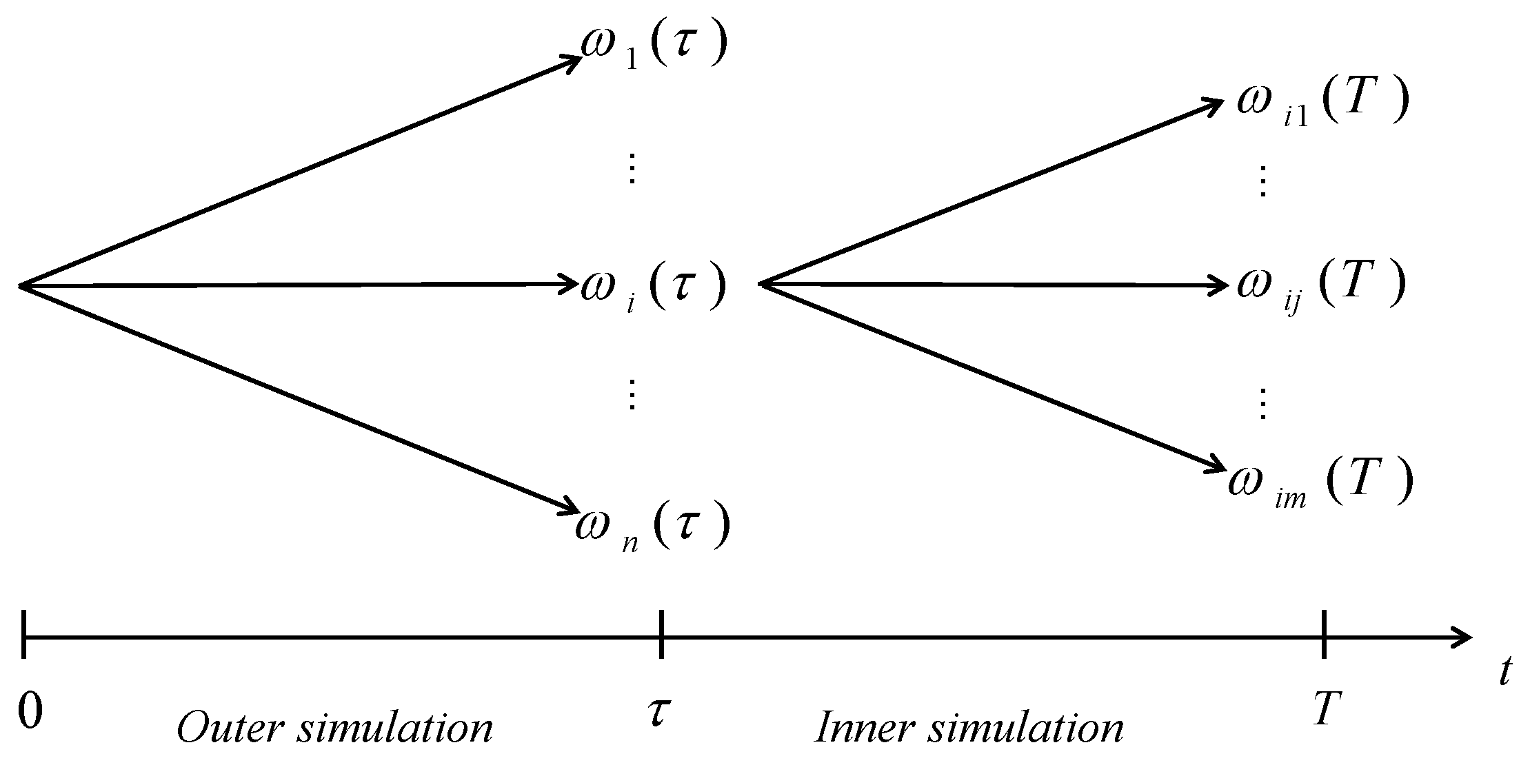
11]. Usually, MC generates the possible scenarios of risk factors in the future and calculates potential loss under each scenario. Among them, the nested simulation framework, proposed by [
12], is purported to simulate the risk factors between any future time intervals, and evaluates the corresponding loss of a system to measure the risk. Basically, nested simulation includes the outer simulation, that generates multiple scenarios of risk factors, and the inner simulation, that generates and calculates the possible system loss in each scenario. It builds up the framework of risk estimation for a system. However, it also encounters trouble in a huge system problem because the required computational effort is too large to obtain reliable results. To solve this problem, related literature discusses the balance of computational effort between outer simulation and inner simulation. Furthermore, some papers, such as [
12,
13,
14,
15], have tried to improve the estimation efficiency or accuracy.
One marked stage of improvement comes from [
16]. This paper considered portfolio risk estimation in financial engineering and used regression to fit the surface of portfolio loss, given the risk factors. Several papers proposed related models based on this framework [
17,
18]. The risk estimation via regression can relax the computational requirement by substituting the inner simulation by a pre-trained regression. Of course, because of the complexity of a system, the performance of risk estimation via regression is problem-dependent and the selection of basis function is of great importance. Intuitively, the appropriate selection of basis function becomes harder for complicated portfolios, such as a portfolio with several derivatives trading in the financial market, because there exists high non-linearity in this system (portfolio) with respect to risk factors [
19,
20].
In this paper, we discuss the risk estimation problem under the framework of portfolio risk management and focus on the basis function selection problem in risk estimation via regression. Portfolio risk management with a complicated structure (including special financial products, such as derivatives) can be a good example of the complex systems we are interested in. Furthermore, we considered a portfolio having risk factors following the Lévy process, which is a type of more generalized stochastic process that has become a newly applied modeling perspective in finance and many other fields. Instead of the polynomial basis function, that is supported by the theory of functional analysis and widely used in the existing literature, we propose a stylized model that is derived by considering artificially simplified risk factors, coupled with the closed form of derivative price. We argue that portfolio loss with simplified risk factors can explain, or cover, the non-linearity of portfolio loss under the Lévy process in most cases. The simplified loss is easy to derive and can be selected as the basis function. Finally, we describe the related methods to test the efficiency of the stylized model and examine the performance of the stylized model in numerical examples.
This paper is organized as follows. In
Section 1, we give a brief introduction of the background and related literature. The stylized model proposed in this paper is illustrated in
Section 2, including the efficiency testing of the proposed model.
Section 3 designs the numerical example to show the performance of the proposed model.
Section 4 concludes this paper and shows the potential future research.
3. Numerical Examples
In this section, we describe the four numerical examples we designed to examine the performance of the stylized model in estimating the risk measure. Still, we assumed that the underlying assets of financial derivatives follow the Lévy process and used the European option as the example of derivatives. So the underlying asset price at time
t, denoted as
, is the vector of risk factors in this example. Take the Variance Gamma (VG) process and the Normal inverse Gaussian (NIG) process as the dynamics of the derivatives’ underlying assets. We considered the following four portfolios in
Table 1 and
Table 2. In each numerical example, we evaluated the estimation performance of Value-at-Risk (VaR) by different choices of basis function. VaR of any random variable
X given
, denoted as
, is defined as
Suppose that the initial prices of underlying assets are denoted by
, risk-free interest rate
, and the maturity of all options
. The risk horizon is
year. There are 4 portfolios considered and each of them consists of one long European call option with underlying assets
and strike price
, one short European call option with underlying assets
and strike price
, and one short call option with underlying assets
and strike price
. The parameters of options in portfolios are shown in
Table 1. The parameters of underlying assets are shown in
Table 2.
Given the parameters setting above, we built our experiments, including the following two procedures. The first part is the training procedure. Given
, we replicated our numerical experiment
times. For each replication, let
M be the number of sample paths of risk factors we generate in the outer simulation for each replication. Here, we set
M = 500, 5000, 50,000, 100,000, respectively. For inner simulation, we set the number of simulation paths as
. Therefore, we have
M sample paths, or scenarios. So, the corresponding portfolio loss in
i-th scenario,
, which is the element of
in Equation (
3) can be computed. The basis functions
are selected according to the description of Basis 1 through to Basis 7. The parameter
r can be estimated by ordinary least square (OLS), given the portfolio loss and basis, denoted as
. The second part is the testing procedure. Set testing sample size
N = 10,000; that is, we generated
N scenarios for each replication to calculate basis. Given the
, we can estimate the portfolio loss. Then, the risk measures
can be estimated,
. The true values of VaR are not available in these numerical examples. We used nested simulation to estimate them. The computational budgets for
were
,
, and
.
The stylized model assumes that the underlying assets follow the Geometric Brownian Motion (GBM) with estimated volatility. Here we may have two ways to estimate it in the numerical examples. Firstly, one can calculate the volatility of the Lévy process to match the one in GBM. For example, consider the VG process as an example, its variance
. The calculation is straightforward for the stochastic process with independent increment. Alternatively, we can estimate the volatility from the simulated underlying asset price. This is widely applied in real applications. According to [
24], given
n samples of underlying asset price at time
T,
, the volatility
in GBM can be estimated by the following procedure:
where
.
For evaluation and comparison of estimation performance using different basis functions, we calculated the relative root mean square error(rRMSE) to show the results in
Table 3,
Table 4,
Table 5 and
Table 6. The rRMSE is calculated using the following equation:
Table 3,
Table 4,
Table 5 and
Table 6 show the rRMSE of estimated
, where
, respectively. Seven different basis functions were tested in the experiments. In general, the estimation became harder if
increased, given the fixed sample budget in the training parts for all the basis functions. So, all the tables show that the rRMSE increased as
increased in most cases. For comparison, 7 basis functions were divided into three groups with similar lengths. The rRMSE with the blue color was the best basis, based on the rRMSE of estimated
. Group 1 consisted of Basis 1 and Basis 2. Basis 1 is the simplest stylized model that only contains the first-order term of B–S price. Basis 2 contains both the linear term and the second-order term of risk factors to capture the high non-linearity of portfolio loss with respect to risk factor. A basis function with only a linear term of risk factors showed really bad performance in all settings, so we excluded it. Group 2 consists of Basis 3, Basis 4, and Basis 5. All the basis functions were designed based on Basis 2 and another different basis function. Basis 3 considers the stylized model. Basis 4 considers the higher order of risk factors. Basis 5 was designed according to [
16]. Inspired by the payoff function of European call option, it tries to capture the non-linearity by
. Group 3 consists of Basis 6 and Basis 7, in order to evaluate the estimation performance of higher order basis functions.
As these tables show, basis functions with the stylized model (Basis 1, Basis 3 and Basis 6) performed better than others in most cases. Furthermore, if we compare each group, the basis function with the stylized model performed better. For comparison among groups, the basis functions
(Basis 5 and Basis 7) were worse than the basis function with the stylized model, but much better than the polynomial basis functions (Basis 2 and Basis 4). Specifically, the estimation performance was surprisingly good with only one stylized model (
). Except for portfolio 3, all rRMSEs were around 0.15%. Meanwhile, little improvement was shown in Basis 3 and Basis 6, compared with Basis 1, in some portfolios. For example, there was nearly no improvement of Basis 3, compared with Basis 1, in portfolio 2 with
, and 0.004% improvement of Basis 5, compared with Basis 1. This also shows the efficiency of the stylized model as basis function in regression Equation (
3).
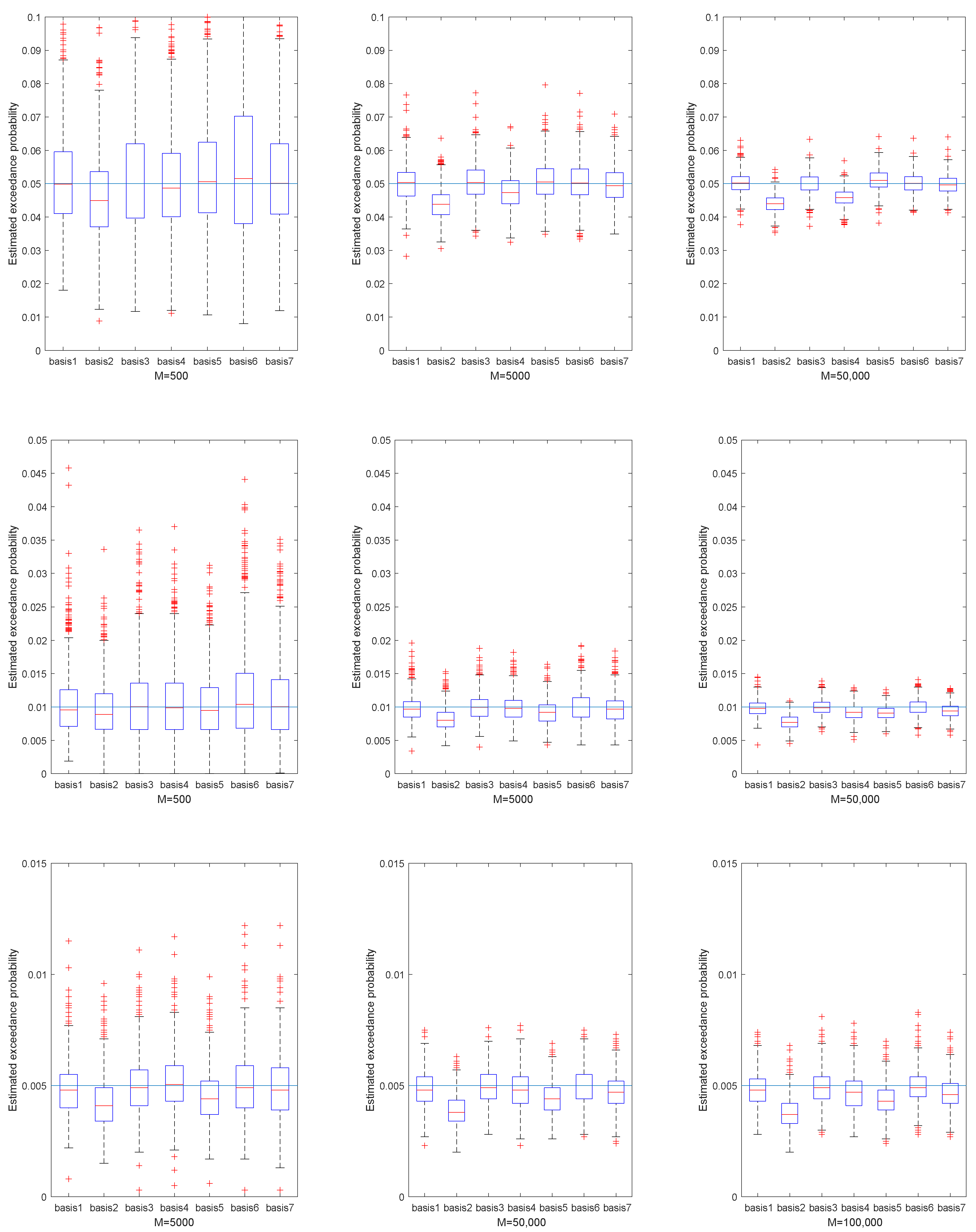
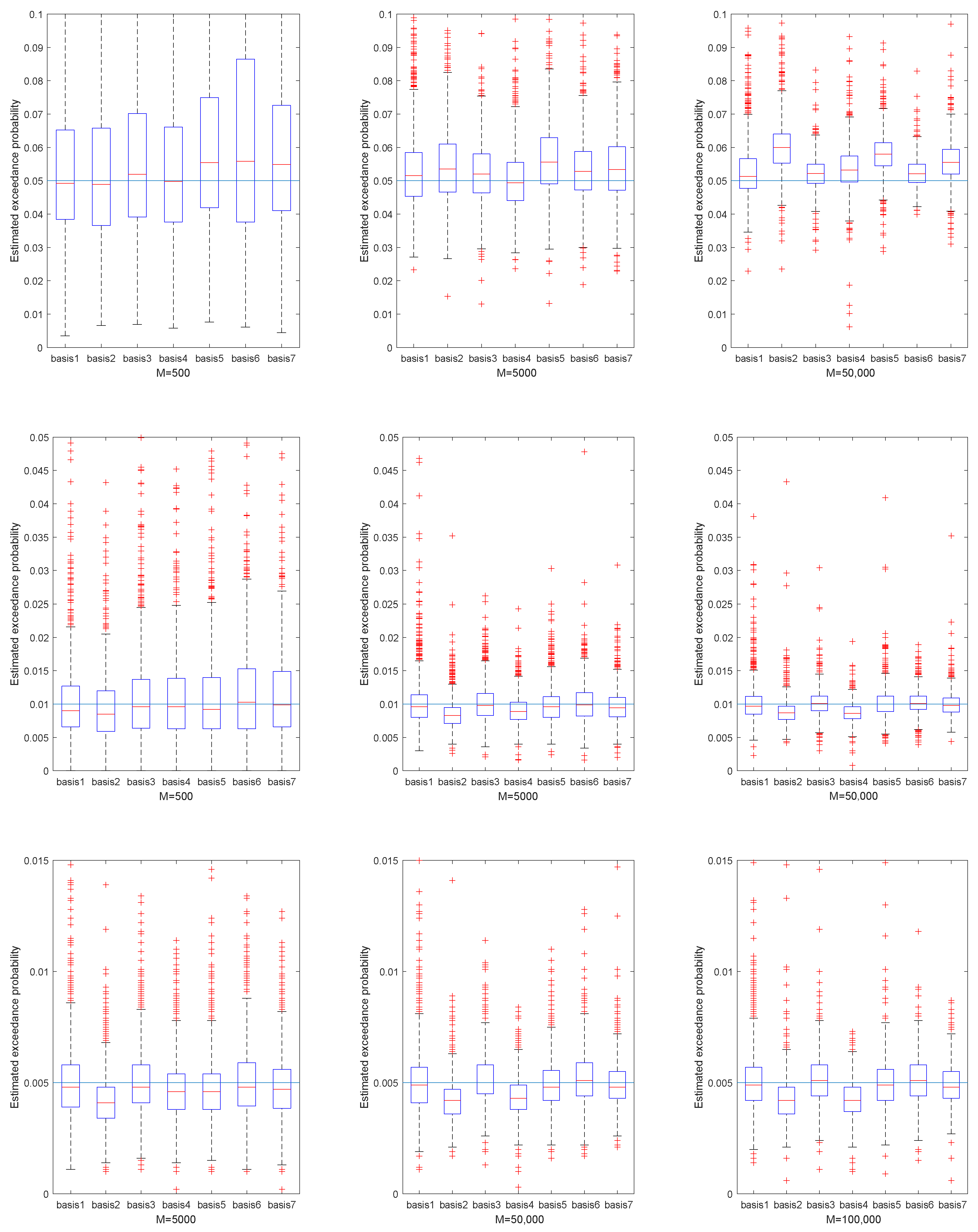
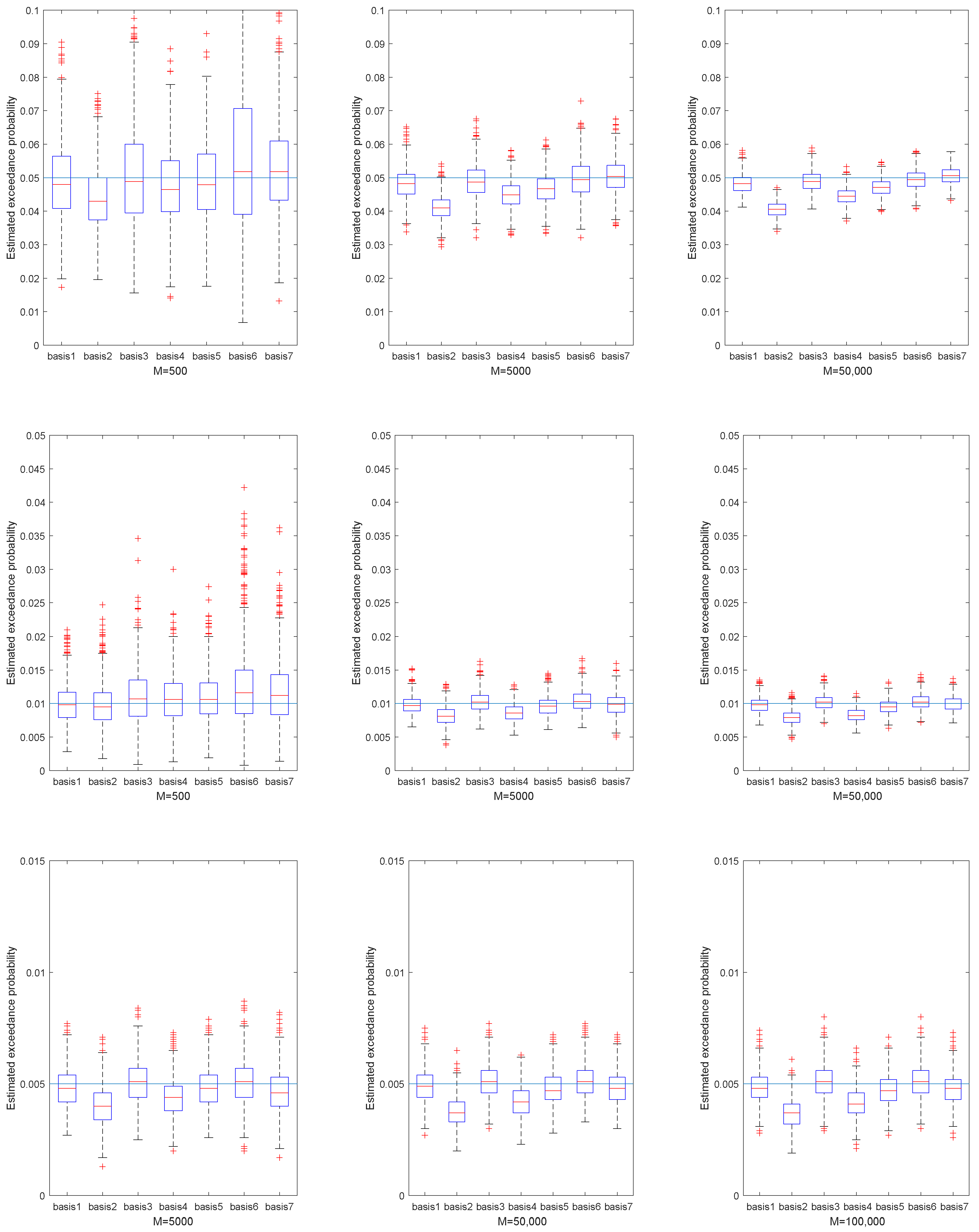
Figure 2,
Figure 3,
Figure 4 and
Figure 5 represent the estimated exceedance probability, given estimated
, in the four portfolios, respectively. The red line of each box plot is the median of estimated
in
H replications. The light blue line is the true exceedance probability. As the training sample increased from
M = 500 to
M = 50,000 for
, and from
M = 5000 to
M = 100,000 for
we see better estimation results of exceedance probability. Specifically, the estimation results in
Figure 4 fluctuated much more than in
Figure 5, because the underlying NIG process had larger variance. So, estimating the
in portfolio 3 was relatively harder than in portfolio 4. Similarly, if we compare the median of estimated exceedance probability, the basis with the stylized model performed better than the others. Still, we did not observe large improvement from Basis 3 and Basis 5 compared to Basis 1 in most cases.


