Abstract
The adoption of all-electric vehicles (EVs) has grown rapidly in the transportation industry, particularly for urban parcel deliveries. However, the limited driving range of EVs and the high investment cost of establishing charging infrastructures are still the holdbacks to routing these EVs. In this paper, we present the vehicle routing problem of a mixed fleet of EVs and conventional vehicles (CVs) via intermediate depots as an alternative strategy to address the challenges, with CVs delivering parcels from the central depot to intermediate depots and EVs delivering parcels from intermediate depots to customers. In addition, we propose an intelligent dispatching scheme to allow EVs to be used for multiple routes. A two-phase approach is developed to first cluster the customers to the intermediate depots and then route the mixed fleet. The strategy is implemented for both small- and large-sized instances, and the results show that using an intelligent dispatching scheme can significantly reduce the number of EVs used. Furthermore, the use of smaller-range EVs is also investigated., and a discussion of potential implementation issues is provided.
MSC:
90-10
1. Introduction
Due to the concerns about environmental pollution and an energy crisis, increasing efforts have been put into the research of green logistics strategies and operations. The adoption of all-electric trucks, or EVs in general, has become one of the key addressees of green logistic activities, especially for urban logistics. More and more EVs are being deployed by logistics companies, i.e., UPS, FedEx, and DHL [1], because of their positive effects on promoting urban sustainability while also reducing greenhouse gas emissions. However, the limited driving range of EVs, the long charging time, and the high investment cost of establishing charging infrastructures remain barriers to EV deployment. A typical EV can drive 75 to 125 miles with a fully charged battery [2,3,4]. However, this range can be significantly shortened by cold temperatures and road conditions [5,6]. Since the daily driving needs of urban logistic services are from 150 miles to 250 miles, a single charge of an EV is not sufficient to complete the entire service route. Therefore, the proper establishment of the charging infrastructure and visits to charging stations are needed.
Different types of charging techniques are available for EV recharging, including conductive charging, inductive charging, and battery swapping. The conductive charging, for which charging infrastructure is required, is classified into different levels of charging technologies by the level of power that they deliver to the battery pack, namely Level 1, 2, 3, and DC fast chargers as presented in Table 1 [4]. The cost of establishing charging stations depends on the technology used. Level 1 and 2 charging stations are inexpensive, with a cost of a few hundred for Level 1 and prices ranging from USD 2000 to USD 6000 for Level 2 [7]. On the other hand, Level 3 and DC fast charging stations cost at least USD 50,000 per station. Moreover, according to the report [4], the average EV truck costs USD 308,000, which is roughly USD 200,000 more than the cost of a comparable diesel CV truck. Despite the predictions that the cost of an EV will fall by more than half by the year 2030, the high cost of the charging infrastructure may increase the industry’s resistance to adopting EVs.

Table 1.
Classification of chargers for EVs.
Because of the benefits of EVs, more and more efforts are being made in the industry to address the challenges of EV adoption. In general, there are two existing strategies for incorporating EVs into fleets. One option is to replace all CVs with EVs. Another option is to consider a hybrid fleet of CVs and EVs. EVs are always assumed to be charged en route, using fast charging technology in existing works, and the capacity of the charging stations is unlimited. This type of assumption, however, may result in high costs for establishing an adequate charging infrastructure as well as congestion at charging stations with a limited capacity. Moreover, the price of an EV is closely related to the size of its battery, with the unit cost of the battery being USD 400–600 per kilowatt hour (Kwh) [4]. The larger the battery pack, the longer the travel distance. EVs with larger battery packs are significantly more expensive than those with smaller battery packs. However, in existing works, a mid-size EV is typically considered for parcel delivery. The possibility of using small-size EVs needs to be further explored.
In this paper, we propose an alternative strategy for adopting EVs in a mixed fleet by introducing additional intermediate depots on top of the central depot to establish a reasonable number of charging stations and consider using EVs with shorter ranges. CVs are primarily used to transport parcels from the central depot to intermediate depots, whereas EVs are only used to transport packages from intermediate depots to customers. For comparison, EVs with large and small travel ranges are deployed. It is also assumed that EVs can only be charged at designated intermediate depots and that they can be used for multiple routes. Partial charge for EVs is also permitted at a charging station located at an intermediate depot. Moreover, our strategy incorporates an intelligent dispatch scheme to route EVs at an intermediate depot, where EVs can depart from the same depot at different times so that the number of chargers needed at a charging station may be properly controlled and the possibility of congestion occurrences at a charging station may be reduced. To our best knowledge, none of the works that are available in the literature on EV routing problems take into account the flexibility of the departure times of EVs. Letting EVs leave the depot at various times allows them to be reused for multiple routes. By incorporating this feature, this paper delivers an efficient operational and routing plan.
The remainder of this paper is structured as follows: Section 2 includes a review of the related literature. Section 3 presents in detail the proposed strategy for introducing intermediate depots and incorporating an intelligent dispatch scheme, as well as a two-phase heuristic developed to be implemented for this strategy. Numerical experiments are conducted, and the obtained results are presented in Section 4. Section 5 includes a case study that demonstrates how to implement our proposed strategy in practice. Our strategy is then expanded in Section 6 to cover the case with more realistic settings. Finally, the conclusions and future plans are provided in Section 7.
2. Literature Review
The vehicle routing problem (VRP), which was originally introduced by Dantzig and Ramser [8], is one of the classic problems in transportation and logistics. The VRP designs proper routes for a fleet of vehicles visiting a set of customers with the objective to minimize the total transportation cost. The VRP with a time window (VRPTW), which is an important extension of the VRP, takes into account the practical requirement that customers must be visited within a certain time frame [9]. The capacitated VRP, considering the limitation of the cargo capacity, is another remarkable extension of the VRP [10]. The VRP using CVs as the mode of transportation has been studied for many years until the growing negative impact on the environment forces the use of alternative fuel vehicles, such as EVs.
Compared to CVs, EVs have the advantage of being powered by clean, sustainable, and renewable energies. However, EVs are limited by their short driving range and they may visit recharging facilities en route, which make the routing problem of EVs different from the traditional VRP using CVs. As routing models using vehicles powered by alternative fuels, e.g., electricity and hydrogen fuel, have just developed in recent years, there is continuing need to enrich related studies. Lin et al. [11] presents a survey on the existing work of such routing models. When a VRP is formulated for any alternative fuel vehicles, it is called a green VRP (G-VRP) problem, while an electric VRP (E-VRP) focuses on EVs. Erdoğan and Miller-Hooks [12] propose the G-VRP, which considers the limited vehicle driving range and the limited refueling infrastructures. It allows the vehicle to visit one or more refueling facility during the route. However, the refueling time is assumed to be fixed. The capacity constraint and time window constraint are not included in the model formulation. As an extension of the G-VRP, Schneider et al. [13] introduced an electric VRP with time windows (E-VRPTW), which takes into account additional constraints on vehicle capacity, customer time window, and flexible recharging time. They also designed a heuristic based on a hybrid variable neighborhood search (VNS) and Tabu Search (TS) to solve the proposed model. Ding et al. [14] investigated the nonlinear energy consumption behavior of EVs and proposed the EVRPTW based on driving cycles (EVRPTW-DC) to minimize the overall costs of distance, recharging, and time window violation. An adaptive particle swarm optimization algorithm was developed and implemented. The results showed that the incorporation of a nonlinear energy consumption model can lead to a more realistic routing plan.
Other than only using EVs in the fleet, there exists another strategy of deploying a mixed fleet of EVs and CVs in recent studies. Gonçalves et al. [15] study the VRP using a mixed fleet of EVs and CVs to complete pickup and delivery tasks. It is assumed that charging facilities are available anywhere and can be visited whenever they are needed by EVs. The number of charging visits is determined by dividing the total traveled distance by the EV travel range, which is unrealistic. Sassi et al. [16] study the problem of routing a mixed fleet of CVs and heterogeneous EVs (HEVRP) with charging availability en route. HEVRP aims at minimizing the number of employed vehicles and the total cost of operating and charging. Different types of charging stations, time-dependent charging costs, and partial charging possibilities are incorporated. A linear charging scheme with an additional constraint on the maximal grid capacity is considered in HEVRP. Later, the E-VRPTWMF model of routing a mixed fleet of EVs and CVs, considering a realistic energy consumption function that is affected by speed, gradient, and cargo load distribution, is proposed by Goeke and Schneider [17]. An adaptive large neighborhood search algorithm embedded with a local search for intensification is developed to solve the problem. However, EVs are recharged to their maximum battery capacity when visiting a charging station. Hiermann et al. [18] introduce a mixed fleet similar to E-VRPTWMF but with heterogeneous vehicles that differ in transport capacity, battery size, and acquisition cost. Macrina et al. [19] proposed the mixed fleet vehicle routing problem with partial recharging and time windows, taking into account the limitation on the fleet’s polluting emissions.
The literature presented above uses a direct shipping method from the origin to the customers. Additionally, there exists another collection of works within the literature that incorporates an indirect shipping method whereby all or part of the customers’ demands are transferred through one or more intermediate facilities, from the origin to the destination. This type of problem is generally called a multi-echelon routing problem and a special case where only one intermediate facility is involved is called a two-echelon routing problem [20].
The two-echelon vehicle routing problem (2E-VRP) in which the set of depots and the set of intermediate facilities are given is related to our problem. In the 2E-VRP, the decisions include the routing at both echelons, i.e., first echelon from depot to intermediate facilities and the second echelon from intermediate facilities to customers, and the allocation of customers to intermediate facilities. Most of the existing work focuses on its basic version, the two-echelon capacitated vehicle routing problem (2E-CVRP), where both the intermediate facilities and vehicles are capacitated. Perboli et al. [21] discuss several variants of 2E-VRP and present a flow-based model for 2E-CVRP and valid inequalities for it. Crainic et al. [22] address the basic version of 2E-VRP, without providing any mathematical formulation. Instead, the authors design a heuristic by separating the first and second echelon routing problems and then solving both problems sequentially and iteratively. A similar approach with a family of multi-start heuristics is proposed by Crainic et al. [23]. Hemmelmayr et al. [24] introduce an adaptive large neighborhood search heuristic (ALNS) for 2E-CVRP, which is reported to be the best-performing heuristic so far. The main idea of the ALNS algorithm is to apply a destroying operator to remove a subset of customers from the current solution and then a repair operator to insert them back into the current solution to find improving solutions. An exact algorithm is introduced by Baldacci et al. [25], who propose a new integer linear programming formulation that is used to derive both integer and continuous relaxations. They present a bounding procedure based on dynamic programming, a dual ascent method, and an exact algorithm that decomposes the 2E-CVRP into a limited set of multi-depot capacitated vehicle routing problems.
However, unlike the intensively studied 2E-CVRP, little work has been found considering the additional time window characteristics of 2E-VRP. Crainic et al. [26] present a time-dependent formulation of 2E-VRP with consideration of customer time windows and fleet synchronization but no time windows for intermediate facilities. The authors also design solution methods, but no computational experiment has been reported. Both [27] and [28] incorporate time window constraints for intermediate facilities and customers into their problems. Govindan et al. [27] consider a soft time window for both intermediate facilities and customers that can be violated if a penalty is paid, while Grangier et al. [28] enforce them to be visited within their time windows. However, in both papers, the time windows for the intermediate facilities and customers are known as parameters. Moreover, none of the available literature considers the case of unknown time windows for the intermediate depot and how to address this matter in the 2E-VRP. Therefore, this is one aspect that will be addressed in our paper.
3. Routing a Mixed Fleet of EVs and CVs for Customers with Time Windows via Intermediate Depots (MFTW-ID)
3.1. Description of the Strategy
In this section, a new strategy MFTW-ID of adopting EVs in the fleet, using a mixed fleet of EVs and CVs with additional intermediate deports, is proposed to serve a set of customers with time windows. Other than serving customers from a single central depot (CD), a number of intermediate depots (IDs) are introduced. A mixed fleet of CVs and EVs is incorporated, with CVs only available at the CD and EVs only available at IDs. On a typical day, packages are either delivered to customers directly by a CV from CD, or to IDs first and then EVs are deployed to deliver packages from IDs to customers. Therefore, a customer can be visited by a CV from the CD or an EV from an ID within its time window. The time window and demand of a customer may change from day to day. Due to the flexibility of customers, it is complicated to pre-determine whether a customer will be served by a CV or an EV statically. Therefore, an average scenario on a single day is first considered in this section to present this strategy.
A customer is feasible for an ID when both of the following conditions are satisfied: (1) the roundtrip distance between the customer and the ID is not larger than the maximum travel distance of an EV, and (2) the customer’s time window is satisfied by the vehicle’s arrival time from CD via the ID. In this scenario, customers are assumed to be feasible to at least one ID. A mixed fleet of CVs and EVs is deployed in such a way that all customers are served by EVs deployed at IDs while CVs are used only between CDs and IDs. Therefore, there are two levels of routing problems. One is CV routing from CD to IDs, and the other is EV routing from IDs to customers. Meanwhile, other than allowing EVs to be charged at additional charging stations en route, it is considered that charging for EVs is only allowed at IDs. Figure 1 presents an example to illustrate this scenario. As shown in Figure 1a, there is a CD and five IDs. Each ID has two key functions, one is to serve a defined area of customers as indicated by the circle in the figure, and the other is to serve as an EV charging station. CVs are used to complete delivery services from CD to IDs (ID1 to ID5). Specifically, for this example, ID1, ID2, and ID5 are served by CV1 while ID3 and ID4 are served by CV2. Once the cargo is delivered to IDs, EVs are dispatched to serve customers within the defined area of each ID. EVs start from IDs and return to the same ID after service. Looking more closely at ID1, a total of five customers are served by two EV routes, as shown in Figure 1b. In this case, since EVs can only be recharged at an ID, it is assumed that the number of chargers at an ID is not restricted and there is no congestion or waiting at the charging stations. An estimate of the customer locations will be provided in this problem to determine the routing plans.
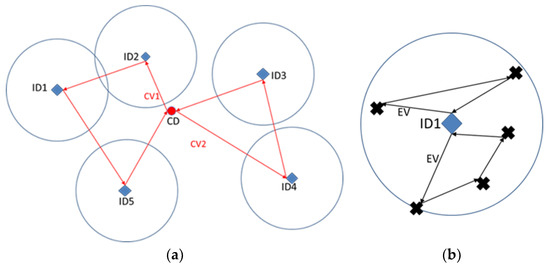
Figure 1.
(a) Strategy with intermediate depots assuming customers are in the range of IDs. (b) Customers assigned and routes generated at ID1.
A two-phase approach is developed for this strategy, where the first phase improves the solution of customer-to-ID allocation, while the second phase determines the routing of the mixed fleet. Based on the first-phase clustering of customers to IDs, each ID is considered a “Big-customer”, with a demand equal to the sum of the demands of the customers assigned to it. The second phase includes two types of routing problems. One is the CV routing problem formulated between CD and IDs, and the other is the EV routing problem formulated between each ID and its assigned customers. Figure 1a presents an example of the CV routing problem from CD to IDs, and Figure 1b is an example of the EV routing problem from ID1 to its customers. In both routing problems, the time window of each node and the capacity of vehicles are taken into consideration.
3.2. First-Phase Clustering
The first-phase clustering aims to generate customer-ID allocation solutions, which are used to decompose the second-phase mixed fleet routing problem into several independent VRPs of a single vehicle type and a single depot. A customer can be assigned to an ID only if the following two conditions are satisfied: (1) the customer is within the range of the ID, and (2) the customer’s time window is satisfied by the arrival time from the CD via the ID. In the current scenario, customers are assumed to be feasible to at least one ID. Knowing the set of customers assigned to a specific ID, the ID is then transformed into a Big-customer for CD, with new demands and time windows determined by the assigned customers. The new demand equals the sum of the demands of the customers assigned to the ID. The initial time window of the ID is the entire timespan, and the new time window only affects the latest time of visiting the ID. The latest time is determined by taking the smallest value of a customer’s latest time and subtracting both the travel time from the ID to this customer and the service time at the ID for all customers assigned to the ID.
The initial clustering follows a distance-based rule, as introduced in Crainic et al. [22] that a customer is assigned to its nearest ID. The assignment must also satisfy the potential restrictions at IDs in terms of capacity and fleet size. The resulting two types of VRP subproblems are solved independently, and the total traveled distance of the second-phase routing is calculated. The following Algorithm 1, which is implemented in Java, presents a heuristic developed to improve the initial clustering.
| Algorithm 1 The improving procedure of first-phase clustering | |
| (0) | Initial clustering of assigning each customer to its nearest ID; solve second-phase routing problem and calculate the global cost of current clustering as the current best solution |
| (1) | Sort customers, which can be assigned to multiple IDs, by the difference in the distance between the customer and its nearest and second-nearest IDs in ascending order, let it be the list |
| (2) | for ( in ), start with the first customer, |
| (3) | Consider total customers in sequence (); Assign customer(s) from to to its second-nearest ID; Update clustering |
| (4) | if the new clustering is not feasible then |
| (5) | Consider the next customer(s) in and restart Step (3) |
| (6) | else then |
| (7) | Transform IDs to Big-customers for CD and formulate CV routing problem (CVRP); |
| Formulate a set of individual EV routing problems (EVRPs) from each ID to its assigned customers; | |
| Solve CVRP and EVRPs and compute the global cost of the new clustering; compare it to the current best solution | |
| (8) | if the new cost is better then |
| (9) | update the current best solution as the new cost, and restart Step (3) from the next customer in the list |
| (10) | else then |
| (11) | Remain the current best solution and restart Step (2) from the next customer in until a stopping criterion of the number of iterations or computing time is reached |
The initial clustering of ID1 and ID2 shown in Figure 1a is presented in Figure 2a. Each ID and its associated customers are marked as the same color, i.e., black for ID1 and green for ID2. By applying one iteration of Algorithm 1, the change in the customer assignments is generated and presented in Figure 2b in that a customer is moved from the ID1 cluster to the ID2 cluster.
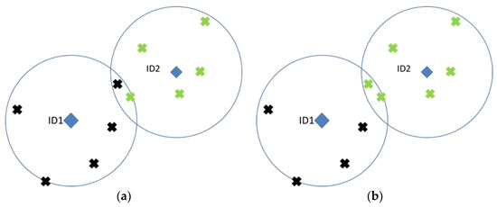
Figure 2.
(a) Initial clustering. (b) A customer’s color changes from black to green after applying Algorithm 1.
3.3. Second-Phase Routing
While the first-phase clustering assigns customers to IDs, the second-phase problem deals with the routing problems of the mixed fleet. Two types of routing problems are observed in this phase. One is CV routing from CD to IDs, and the other is EV routing from each ID to its respective customers. As a result, there is one CV routing subproblem and a set of EV routing subproblems up to the number of IDs. This section first formulates a mathematical model for the EV routing problem and then explains how it can also be applied to the CV routing problem. It then proposes an alternative heuristic to solve the EV routing problem, where an intelligent dispatch scheme can be added.
3.3.1. Mathematical Formulation for EV Routing Problem
A typical E-VRPTW aims to minimize the total distance of routing a set of EVs that depart from the depot and visit a set of customers within pre-specific time intervals. It allows EVs to be charged at charging stations en route when needed, and return to the depot before reaching the safe power level. Additionally, the limited freight capacity of EVs is incorporated into the E-VRPTW model [13].
Similar assumptions are made in our E-VRP regarding the customer time windows and vehicle capacity limitations. An E-VRP exists for any ID that has at least one customer. EVs depart from an ID at the same time and return to the same ID once their route is completed. EV charging, on the other hand, is only available at the ID where an EV must return before its battery runs out. It is also assumed that enough chargers are available to serve the EV whenever it arrives and that EVs travel at a constant speed. To describe our model, we use similar notations in Ding et al. [14] for sets, variables, and constants, as summarized in Table 2. Our model incorporates partial charge by introducing decision variables and . specifies the battery level of EV arriving at the node , while indicates the battery level of EV leaving from the node. If node is a charger station, an EV is not necessarily charged to the full battery capacity . Therefore, only the difference between and needs to be recharged. The charging time, which depends on the new charging amount, could possibly be reduced.
Table 2.
List of notations in the E-VRP model.
We then formulate a mathematical model with the following objective function:
Subject to the following constraints:
The objective function is, as expressed in (1), to minimize the total travel distance. Constraints (2) ensure that each customer must be visited exactly once. Constraints (3) ensure that the number of employed vehicles does not exceed the number of available vehicles. Constraints (4) establish the flow balance so that the flow entering a node is equal to that exiting the same node. Constraints (5) and (6) ensure that each vehicle departs from and returns to the depot. Constraints (7) restrict the initial load to the maximum load capacity of a vehicle. Constraints (8) enforce the fulfillment of demand at customer nodes and ensure a nonnegative load for a vehicle upon arrival at any node. Constraints (9) make sure that EVs leave the depot with a full battery, while Constraints (10) restrict the battery to being within the range of minimum and maximum levels. Constraints (11) set the battery level at a node succeeding a previous node following a linear battery consumption behavior. As presented in Constraints (12), an EV maintains the same battery level at a customer node. Constraints (13) guarantee that the remaining battery of an EV leaving from a customer node should at least allow it to go back to the depot. The departure time of any vehicle from the distribution center is set to be zero, as constrained in (14). Constraints (15) enforce that each node is visited within its time window, and Constraints (16) guarantee the time feasibility between successive nodes. It is ensured in Constraints (17) that the arrival and departure times at any node are within the maximum time span. Moreover, the return time of any vehicle to the distribution center must be within the maximum time span as presented in Constraints (18). Constraints (19) illustrate the relationship between the arrival and departure times at a node such that the departure time is composed of the arrival time and the service time. The service time is a given for a customer, and the recharging time is calculated at a fixed recharging rate for a recharging station, as presented in Constraints (20).
This E-VRP model can be applied to CV routing from CD to IDs, in which CD is the depot, the customers for CD are the Big-customers transformed from IDs, and CVs are vehicles that have no battery limit. Similar to a customer, a Big-customer is associated with a newly generated demand and time window. The E-VRP model is revised as C-VRP to solve the CV routing problem by removing battery restrictions and battery-charging-related constraints, i.e., Constraints (10)–(13), and resetting the service time at a charging station to be zero in Constraints (20).
3.3.2. Heuristic of EV Routing
The assignment of customers to IDs from first-phase clustering serves as the input for second-phase routing. Because transforming an ID into a Big-customer aggregates the demands of customers assigned to this ID as the new demand, more CVs and/or CVs with a larger cargo capacity may be required to complete CV routing. On the other hand, an EV can intuitively serve another route after returning to its ID and being charged. We say that the EV has completed a route and is now being used for another if an EV returns to the ID for charging before departing again to serve customers. As a result, the same EV could be used for multiple routes, but the starting times of the routes are not pre-defined. To avoid requesting additional resources and potentially improve vehicle utilization, we also propose a heuristic method for the problem. We include an intelligent dispatch scheme that allows EVs to depart from IDs at different time points so that an EV can be used for multiple routes while additional Big-customers should be generated, assuming the total time span of service to customers is eight units. When using the mathematical model in Section 3.3.1, EVs leave the depot at time zero. In the heuristic, EVs leave the depot at different time points depending on the dispatch interval . If is four units, then a set of EVs leave the depot at time zero and another set leaves at time four. Similarly, if is two units, there will be four sets of EVs leaving the depot at times zero, two, four, and six, respectively. The minimum value of is one unit. Therefore, the dispatch interval can be as large as the entire time span, i.e., eight units, or as small as one unit.
Figure 3 presents our solution method in a flow chart. For an ID and its customers, an aggregation step first takes place where customers are grouped by their earliest time of service scaled to the intervals of dispatching EVs. Each group of customers is then assigned with a dispatch time point , meaning that for EVs to serve group will leave from ID at . Moreover, a Big-customer is generated for each group of customers and added to the CV routing problem.
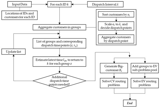
Figure 3.
Overview of heuristic to solve second-phase routing problem.
The next step is to estimate the latest time that EVs should return to ID by estimating the average number of customers per route using the method proposed by Figliozzi [29]. The conditions needed to be checked to see if additional dispatch time points are required because customers may not be served within their time windows when EVs leave the depot at the current dispatch time. A customer , with and , needs time to travel to its corresponding ID . The following two conditions need to be checked: (1) If , customer cannot be served by the vehicle leaving at because an EV is not able to visit this customer within its time window; (2) If , an EV cannot return to its depot in time that customer cannot be served by the vehicle leaving at . If either of the conditions are satisfied, new dispatch time points are required and added, and the list of customer groups is updated. Otherwise, the current group of customers with the associated time of dispatch and time to return is added to the subproblem pool to be solved. Each subproblem in the pool has the following features: an ID, a group of customers, and of EVs, and recharging is only available at the ID. Therefore, each subproblem is an E-VRP problem, as described in Section 3.3.1. The formulation developed in Section 3.3.1 is used to solve the subproblems, and the number of vehicles and their routes will be obtained. As mentioned earlier, in the heuristic, EVs are allowed to serve multiple routes after they return to the depot and get charged if it is necessary. Partial recharging is allowed. By using EVs for multiple routes, it Is possible to reduce the actual number of vehicles that are used.
3.4. Realistic Scenario Considering Outliners
At the beginning of Section 3, an average scenario on a typical day assuming that customers are all within the range and served by EVs from IDs is explained in detail. However, in a general case of the proposed strategy, a customer must be served by either a CV from the CD or an EV from an ID, because a customer may not be feasible to any of the IDs. Therefore, it is necessary to further explore the general scenario of determining whether a customer is served by a CV or an EV.
According to Section 3.1, a customer is said to be feasible for an ID only if both the distance and time window conditions are met. and are the distance and travel time between two nodes in the network, respectively. Condition (1) is satisfied when , where is the threshold. Condition (2) is satisfied when . A matrix is introduced to present if a customer can be assigned to an ID. Let be an element in , where are two nodes in the network. Only when one of is a customer node and the other is an ID node, the value of could be either 0 or 1. Otherwise, the value of is always 0. When both conditions, the value of is 1. Otherwise, equals 0. If a customer is not feasible to any of the IDs, i.e., , this customer is an outliner and should then be served directly by a CV from CD. The above process to determine whether a customer is an outliner is shown in Figure 4.
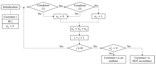
Figure 4.
The process to determine whether a customer is an outliner.
After determining the subsets of customers to be served directly by CVs or by EVs, the subsets of customers being served by CVs are added to the CV routing problem; on the other hand, the subsets of customers being served by EVs from their associated IDs can formulate EV routing problems. Additionally, both types of routing problems can be solved as described in Section 3.3. Figure 5 presents the overall flow chart of our proposed two-phase approach while considering the customer outliners.
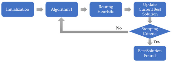
Figure 5.
The overall procedure for the two-phase approach.
4. Experimentation
This section presents the numerical experiments conducted to test the proposed strategy. We create our instances from those used for E-VRPTW by Schneider et al. [13]. Different numbers of customers are served in these instances. We use the instances with 15 customers and 100 customers, representing the small and large-size instances, respectively. Given an instance of Schneider et al. [13], with a depot, 20 charging stations, and 100 customers, we re-define the charging station locations as the locations of intermediate depots for our problem. Instances are solved by the proposed model and heuristic implemented in Java on a desktop computer with an Intel i5 2.67 GHz Processor with 4 GB RAM, running Windows 7 Professional, and the available resources in the Center for Computational Research (CCR) at the University at Buffalo.
4.1. Analysis of Second-Phase Routing
To solve the second-phase routing problem, we use two methods, as proposed in Section 3.3. Mathematical models for CV routing and EV routing are implemented first, and a heuristic approach is further implemented for EV routing. Additionally, directly using the mathematical formulation for EV routing is equivalent to using the heuristic when the dispatch interval is the entire time span.
When using the heuristic, the EV routing problem is solved with different dispatch intervals . If the total time span is , then the number of intervals can range from 1 to . When , for the EV routing subproblem, EVs leave their ID at time 0 and can only serve 1 route. The charging technology used at an ID can either be a slow charger over the night or a fast charger in less than 0.5 h. Moreover, each ID is transformed into one Big-customer for the CD, with new demands and time windows determined by all customers assigned to this ID, as described in Section 3.2. In the case when is greater than 1, customers assigned to an ID are split into subsets. A total number of Big-customers are generated for this ID, one for each subset of assigned customers. EVs are dispatched at time points from their ID. After an EV returns to its ID after visiting customers on a route, it may be recharged at the depot depending on its current battery level. If the same EV is going to serve the next route, and it has sufficient battery to cover the next route, it is not necessary to be charged; otherwise, this EV needs to be charged to the least battery level required to serve the next route. Fast charge technology is used to enable this feature. Examples of two different cases are presented in Figure 6. In Figure 6a, there are two routes of the same ID. Either of them is associated with a time window of the depot and a travel distance. The maximum travel distance of an EV is 79.7. If an EV leaves at time 0 and returns at time 552.6 after completing the route with a travel distance , the same EV can continue to serve without being charged at the depot. This is because the total distance of and , i.e., 58, is less than the maximum travel distance of the EV. However, in Figure 6b, after the EV completes the route , it needs to be charged before continuing to serve the route because the sum of and , 82.8, is greater than 79.7.
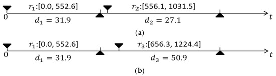
Figure 6.
Examples of using an EV for multiple routes: (a) no need to charge at a depot; (b) need to be charged at a depot.
Take instance c103_15 as an example of a small-sized instance; 1 customer is identified to be served by CV from CD while the rest are served by EVs from IDs. A total of 4 IDs exist, and the number of customers assigned to is 3, 5, 3, and 3, respectively. Results for EV routing in second-phase routing are presented in Table 3. With the same customer clustering from the first phase, both the E-VRP model and heuristic method are applied to the EV routing subproblem, while the C-VRP model is implemented for the CV routing subproblem. The second and third columns provide the number of EVs required and the routing distance at each ID, as determined by the optimal solution of the E-VRP model. For the heuristic method, dispatch interval is selected in such a way that the number of intervals takes values of 1, 2, 4, 8, and 16, as shown in the second row in Table 3. With the same customer clustering, the EV routing problem is solved with a different number of intervals for each ID, and results are also presented in Table 3. Heuristic gives the best solution found in up to 20 iterations. For the same instance, using the E-VRP is equivalent to using the heuristic when the dispatch interval is the entire time span, i.e., only one interval that , and this is observed in Table 3. When there is only 1 interval, i.e., , all EVs leave the depot at time 0. However, when is greater than 1, it means that EVs leave ID at different time points, and the same EV can be used to serve multiple routes for the same ID.
Table 3.
E-VRP and heuristic of EV routing for small-sized instance c103_15.
It is observed from Table 3 that the minimum number of EVs remains the same and the total travel distance of EV routing increases as m increases for this specific instance. The increase in total traveled distance can be explained by the number of customers assigned to each ID being too small and that having multiple dispatch times would force EVs to visit customers in separate routes. Meanwhile, the same minimum number of EVs indicates that an EV is used to serve multiple routes from different dispatch times for an ID.
An analysis is then conducted for the CV routing subproblem using heuristic, since the number of Big-customers is changing along with value and the number of intervals. For the same instance c101_15, the results of CV routing with different value are presented in Table 4. The number of Big-customers generated for each ID increases as increases. This is because customers assigned to an ID are split up into subsets and one Big-customer is generated for each valid subset. While the number of CVs used remains the same, the total traveled distance of CV routing is reduced when increases and has the smallest value when 4 or 8. Therefore, although Table 3 shows that EV routing may not be improved with larger , the CV routing could be improved instead.
Table 4.
Results of CV routing for small-sized instance c103_15.
Similarly, take instance c101_21 as an example of large-size instances. A total of 9 out of 100 customers are determined to be visited by CVs in first-phase clustering and results for EV routing and CV routing with the same customer assignments are obtained with 1, 2, 4, 8, and 16 as presented in Table 5. The results presented in the table are the best found in 100 iterations. It is observed from Table 5 that the total traveled distance of EVs becomes smaller as becomes larger, which indicates that having additional dispatch times helps to give better routes. Additionally, the total traveled distance of EVs can be improved by at most 16.3%. The minimum number of EVs is always greater than or equal to 20 since a total of 20 IDs are available for the instance and each ID is assigned to at least 1 customer. It is shown in Table 5 that the minimum number of EVs decreases as the number of intervals increases. This is because EVs can be used for multiple routes if is greater than 1. Additionally, the number of EVs needed for instance c101_21 can be reduced by up to 7 if the proposed heuristic is combined with the intelligent dispatch scheme. Additionally, since EVs can only be charged at IDs and the possible service time of EVs can spread through the entire time span, the number of chargers at an ID could be potentially reduced.
Table 5.
Results for large-size instance c101_21 with various m values.
As for CV routing, it is shown in Table 5 that at most, 4 additional CVs are required as increases, while the total traveled distance of CVs is reduced by up to 7.3%. This can be explained by the fact that customers are split into more subsets with more dispatch times; thus, more Big-customers are visited by CVs. The overall routing distance including both EV routing distance and CV routing distance is displayed in the last column in Table 5 and it can be improved by 11.7% as increases to 16. The last observation from the experiments is that the larger it takes, the longer the computational time to complete an iteration. This is mainly caused by the longer time to solve CV routing as the number of Big-customers increases when is larger. Therefore, a larger is not entirely beneficial to solving the problem, and a compromise between the value of and satisfactory results is indeed necessary. It is noticeable from Table 5 that the result from and are quite close, whereby both results are slightly worse than that obtained from . However, the time it takes to compute for 4 and 8 is observed to be much less compared to that for in the experiments. Thus, while considering computational efficiency, is selected to obtain results and perform further analysis.
4.2. Results of the Two-Phase Approach
Table 6 reports the results of using the two-phase approach toward large-size instances. The result of a large-size instance is the best found in 100 iterations. As explained in the above section, is applied to obtain results of large-size instances. The instances have three classes of distribution patterns, clustered with a name starting as “c”, random with “r”, and mixed with “rc”. Instances sharing a similar name, i.e., c101_21, r101_21 and rc101_21, have the same time windows but different distributions for customers and are compared as a set. It is observed in Table 6 that, of all three instances in a set, the one with randomly distributed customers has the largest overall distance, as well as the largest individual values of the number of EVs, EV routing distance, number of CVs, and CV routing distance. The smallest overall distance is obtained in the one with clustered distributed customers. Instances of the same distribution, i.e., c101_21, c102_21, and c103_21, are different in terms of the time windows of customers, where c101_21 has the most restricted time windows and c103_21 is the least restricted. Comparing the results of instances with the same distribution, the largest overall distance is found in the instance with the tightest time windows, i.e., c1010_21, while the smallest overall distance is the one with the least restricted time windows, i.e., c103_21. This is valid for three different distributions of customers. Moreover, the individual values of EV routing and CV routing are also smaller when the time windows of customers are more relaxed for the instances with the same distribution.
Table 6.
Results of two-phase approach on large-size instances.
5. Case Study
This section aims to test our proposed strategy with different ranges of EVs and provide a guideline for applying it in a real-world situation.
We use data from instance c101_21 to analyze the flexibility of our proposed strategy. The default maximum travel range of EVs is 79.7 and it will be reduced from 90% to 30% of the default range by a 10% reduction. Figure 7 shows the locations of one hundred customers, one central depot, and twenty candidate intermediate depots.
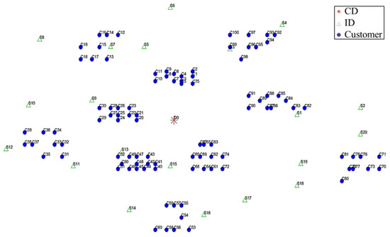
Figure 7.
Locations of customers, depot, and candidates of instance c101_21.
When running the test, it is assumed that the EVs travel at a constant average speed and that EVs of different range limitations have the same speed. We also assume that Level 3 fast charge technology is installed and used at the charging station located at an intermediate depot. For each range of the EVs, the instance is solved by the proposed two-phase approach. Figure 8 presents the initial customer clustering with EVs of a default travel range.
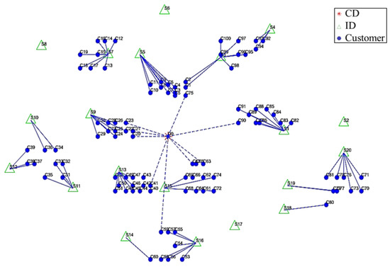
Figure 8.
Initial customer clustering with the default range of EVs.
As shown in Figure 8, customers connected to CD, i.e., , with dash lines are the outliners that are served by CVs from CD, and a total of 9 out of 100 customers are outliners. The rest of the customers are assigned to IDs. Sixteen out of twenty IDs are associated with at least one customer. For each test of a different EV range, the EV routing in the second-phase routing is solved by the heuristic with an intelligent dispatch scheme. The number of intervals is set to be four. The results of each test from the two-phase approach, including the number of outliners, EV routing, and CV routing are presented in following Table 7. The number of outliners is presented in the first column of Table 7, and it can be seen that the number of outliners remains the same as that of the default range for EVs ranging from 90% to 50% of default. This indicates that the current settings of IDs are more than sufficient to serve customers. However, as the EV range is reduced further, the number of outliners increases. When the EV range is reduced to 30%, then 28% percent of customers are outlined to be served by CVs from CD. We decided not to further analyze this test since we are interested in at least 85% of customers being served by EVs from IDs.
Table 7.
Results for instance c101_21 with different ranges of EVs.
It is also observed from Table 7 that the individual values of EV routing and CV routing increase as the range of EVs decreases in most cases. When the range of EVs decreased to 90%, of the default range, the minimum number of EVs, as well as CVs, remains the same, but the traveled distance slightly increases. If the range of EVs further decreased to 80%, 70%, 60%, 50%, and 40% of the default range, the minimum number of EVs increases gradually from 27 to 35, as does the EV routing distance. This can be explained by the fact that an EV with a smaller range has to be recharged more frequently and a smaller number of customers can be visited in one route. Therefore, more EVs are needed to serve customers within their time windows. Furthermore, the impact of the EV range on CV routing is less than that on EV routing, since the increase in the number of CVs and CV routing distance is slower. Compared to about a 27% increase in the EV routing distance, the CV routing distance increases by about 14% when the EV range is reduced to 40% of the default range.
6. Discussions
6.1. Features of an ID
In our proposed MFTW-ID, a customer is visited either by a CV directly from a CD or by an EV from an ID after this ID is served by a CV. An ID serves as the depot and charging station for a set of EVs. There is no limitation on the amount of demand that can be processed at an ID. However, features of fleet size, handling capacity, and demand level at an ID could be further explored.
It is obvious from the results that the fleet size and handling capacity of an ID affect customer clustering. Assuming each ID is associated with a handling capacity , a customer clustering must be feasible to the , meaning that a customer cannot be assigned to an ID if the total demand of customers assigned to the ID exceeds . In this case, even if the customer is feasible to the ID, it cannot be assigned to the ID. Moreover, customer clustering is restricted by the fleet size. An example assuming a system with two identical IDs of 500 units handling capacity and two EVs of 200 units cargo capacity for an ID, and total customer demand of 750 units, a customer clustering of 450 units for one ID and 300 units for the other ID is infeasible since at most 400 units can be accommodated by the two EVs at an ID. The features of fleet size and handling capacity at an ID can be incorporated in Algorithm 1, introduced in Section 3.2, by revising its feasibility check. In addition to satisfying ID conditions in the current Algorithm 1, new feasibility conditions concerning fleet size restriction and handling capacity should all be satisfied for feasible customer clustering in the first phase of the proposed two-phase methodology.
Furthermore, two levels of routing exist in the second phase, and it is necessary to address the synchronization issue between the two levels in terms of time and storage. As described in previous sections, the time window of an ID is determined by the set of customers assigned to this ID. An ID can transform into one or more Big-customers for CV routing from CD, depending on the number of dispatch intervals. However, storage at the ID has not yet been considered. Considering instance c101_21, Figure 9 presents the demand level at each ID when , while Figure 10 shows the fluctuation of the demand level at each ID with the number of dispatch intervals under the same customer assignments to IDs. The dispatch time points are shown as the legend in the figures. It is seen from Figure 9 that when , i.e., the set of customers assigned to an ID is served by a set of EVs all departing from this ID at the same time, the storage requirements at the ID are expected to accommodate the total demand amount of the set of customers. The average demand at each ID is over 100 units. Furthermore, in terms of labor shifts, it indicates that all workers prepare incoming shipments from CD for outgoing shipments to the customer during the same period. In this case, large storage space and sufficient manpower are required to conduct a smooth operation. Comparing Figure 9 with Figure 10 of , it is observed that the fluctuation of the demand level becomes smoother as increases. Considering the case with , the largest demand requirement at ID is 50 for the second and third intervals. This indicates that the storage requirement could be set to be sufficient to cover the largest demand, which is less than 1/3 of the required storage, 170, for . Moreover, workers can prepare shipments during different shifts, and a smaller number of workers could be expected. Therefore, introducing multiple dispatch time points can potentially reduce the requirement for storage and improve labor efficiency. To incorporate this matter into our current strategy, we would suggest two options. One is to add budget constraints at an ID indicating a storage space budget and a labor budget, while the other is to consider such operational costs at an ID as an element in the cost objective function.
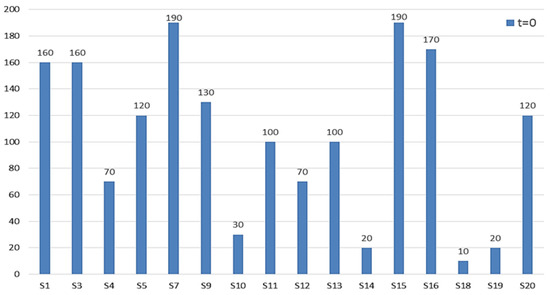
Figure 9.
The demand level at IDs for instance c101_21 with .
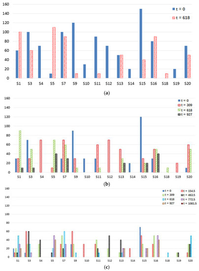
Figure 10.
Fluctuation of demand at IDs for instance c101_21 with (a) ; (b) ; and (c) .
6.2. EV Specifics
The EV routing model used in MFTW-ID assumes a constant travel speed, a constant battery consumption rate depending only on the traveled distance, and fast charging availability at IDs. However, it is necessary to address more realistic assumptions about EVs to implement this strategy in the industry. The travel speed of an EV is not always constant, depending on the battery level, traffic conditions, driver’s behavior, etc. More importantly, the battery consumption rate is affected by different factors, including, but not limited to, the cargo weight, travel speed, road conditions, and weather conditions. The EV battery consumption model, considering vehicle mass, travel speed, and terrain gradient, is introduced by Ding et al. [14], and can be considered an option to implement.
The last matter we would like to address is the charging technology. Although fast charging is enabled for MFTW-ID, Level 2 charging could be implemented. For the same amount of energy, Level 2 charging is known to take a longer time than fast charging. Consider a scenario in which the overall service time of EV routing is 6 h with three dispatch intervals. A set of EVs is dispatched at the beginning of each interval. With Level 2 charging technology, the EVs used in the first interval may be unable to complete the task in the second interval but could be ready for the third interval. The charging time also depends on the battery size of EVs. As analyzed in Section 5, with the incorporation of an intelligent dispatch scheme, small-range EVs, which have smaller battery sizes, can be used for the same problem. Under the same charging conditions, it takes less time to charge a smaller battery than a larger battery. Therefore, by using smaller-range EVs, Level 2 charging technology could become feasible to implement.
7. Conclusions and Future Research
In this paper, we propose a new alternative strategy to adopt EVs in the fleet and the solving methods that are implemented for this strategy. Our proposed strategy consists of optimizing the routing of a mixed fleet of EVs and CVs to minimize the total travel distance. Contrary to existing works that suggest that EVs can be charged en route at established charging stations, we introduce intermediate depots and consider the fact that charging stations are only available at such intermediate depots. Moreover, other than using EVs with larger travel ranges, EVs with smaller travel ranges are employed and tested so that the purchase cost of EVs may be reduced. A two-phase approach is proposed to route a mixed fleet of EVs and CVs by locating additional intermediate depots first, and then routing EVs with charging that is only available at an intermediate depot. Additionally, EVs are possibly used for multiple routes after returning to a depot and being charged, if necessary. We develop a heuristic algorithm to improve the assignment of customers to IDs in the first-phase clustering problem. For the second-phase routing problem, we develop both a mathematical model for E-VRP and a heuristic method with the intelligent dispatch scheme to solve the routing problem of EVs. Both small and large instances are tested by the proposed two-phase approach by implementing the solution methods in Java. It is shown that our proposed method is more suitable for large-size instances, and by using the intelligent dispatch scheme, our strategy can reduce the total number of EVs needed by nearly 22%. Our proposed strategy also aims to solve the cases that may not be solved by E-VRPTW when the maximum travel range of EVs is reduced to a smaller value, which allows cheaper EVs to be adopted into the fleet so that the investment cost of using EVs may be reduced. It is noticeable that reducing the EV range does not necessarily lead to more outliners of customers if the number of IDs is sufficient. Therefore, one of the options for future work would be to explore the efficient planning of IDs in terms of their number and location.
Depending on the status of the current fleet, this strategy can be used to analyze the investment options of introducing additional EVs into the fleet, such as the types/ranges, and estimated number of EVs. Therefore, future work could also explore the influence of the proposed adoption strategy on the investment costs of EVs, including establishing depots, installing charging stations, and purchasing EVs. Additionally, comparisons between different strategies for adopting EVs in the fleet are necessary under different scenarios, including but not limited to battery capacity, charging technology, and energy unit price, to provide better advice on when and how to adopt EVs into the current fleet.
Author Contributions
Conceptualization, N.D.; Formal analysis, N.D.; Methodology, N.D.; Supervision, N.D. and M.L.; Writing—original draft, N.D.; Writing—review and editing, N.D., M.L. and J.H. All authors have read and agreed to the published version of the manuscript.
Funding
This study is sponsored by the Fundamental Research Funds for the Central Universities, Chang’an University (No. 300102220302), and the Shaanxi Province Natural Science Foundation of China (2023-JC-QN-0526), which are greatly acknowledged. The Center for Computational Research at the University at Buffalo is greatly acknowledged.
Data Availability Statement
Not applicable.
Conflicts of Interest
The authors declare no conflict of interest.
References
- International Post Corporation: Green Flash. Available online: http://www.ipc.be/~/media/documents/public/market-flash/green%20issues/gf18.pdf (accessed on 7 August 2017).
- Rhoda, D. 100 Electric Vehicles Begin Their Journey to Save 126,000 Gallons of Fuel Per Year. Available online: http://blog.ups.com/2013/02/08/100-electric-vehicles-begin-their-journey-to-save-126000-gallons-of-fuel-per-year/ (accessed on 17 November 2016).
- Ingram, A. Nissan e-NV200 Electric Vans Join FedEx Trial Fleet. Available online: http://www.greencarreports.com/news/1089878_nissan-e-nv200-electric-vans-join-fedex-trial-fleet (accessed on 17 November 2015).
- CARB Air Resources Board. Technology Assessment: Medium- and Heavy-Duty Battery Electric Trucks and Buses. Available online: https://ww2.arb.ca.gov/sites/default/files/classic/msprog/tech/techreport/bev_tech_report.pdf?_ga=2.223954654.470138175.1676896851-1820634783.1676896850 (accessed on 6 October 2018).
- Botsford, C.; Szczepanek, A. Fast charging vs. slow charging: Pros and cons for the new age of electric vehicles. In Proceedings of the 24th International Battery, Hybrid and Fuel Cell Electric Vehicle Symposium & Exhibition (EVS 24), Stavanger, Norway, 13–16 May 2009. [Google Scholar]
- Tredeau, F.P.; Salameh, Z.M. Evaluation of lithium iron phosphate batteries for electric vehicles application. In Proceedings of the 2009 IEEE Vehicle Power and Propulsion Conference (VPPC), Dearborn, Michigan, 7–10 September 2009. [Google Scholar]
- RMI. EV Charging Station Infrastructure Costs. Available online: http://cleantechnica.com/2014/05/03/ev-charging-station-infrastructure-costs/ (accessed on 21 September 2015).
- Dantzig, G.B.; Ramser, J.H. The truck dispatching problem. Manag. Sci. 1959, 6, 80–91. [Google Scholar] [CrossRef]
- Solomon, M.M. Algorithms for the vehicle routing and scheduling problems with time window constraints. Oper. Res. 1987, 35, 254–265. [Google Scholar] [CrossRef]
- Laporte, G.; Mercure, H.; Nobert, Y. An exact algorithm for the asymmetrical capacitated vehicle routing problem. Networks 1986, 16, 33–46. [Google Scholar] [CrossRef]
- Lin, C.; Choy, K.L.; Ho, G.T.; Chung, S.H.; Lam, H.Y. Survey of green vehicle routing problem: Past and future trends. Expert Syst. Appl. 2014, 41, 1118–1138. [Google Scholar] [CrossRef]
- Erdogan, S.; Miller-Hooks, E. A green vehicle routing problem. Transp. Res. Part E Logist. Transp. Rev. 2012, 48, 100–114. [Google Scholar] [CrossRef]
- Schneider, M.; Stenger, A.; Goeke, D. The electric vehicle-routing problem with time windows and recharging stations. Transp. Sci. 2014, 48, 500–520. [Google Scholar] [CrossRef]
- Ding, N.; Yang, J.; Han, Z.; Hao, J. Electric-Vehicle Routing Planning Based on the Law of Electric Energy Consumption. Mathematics 2022, 10, 3099. [Google Scholar] [CrossRef]
- Gonçalves, F.; Cardoso, S.R.; Relvas, S.; Barbosa-Póvoa, A. Optimization of a distribution network using electric vehicles: A VRP problem. In Proceedings of the IO2011-15 Congresso da associação Portuguesa de Investigação Operacional, Coimbra, Portugal, 18–20 April 2011. [Google Scholar]
- Sassi, O.; Cherif, W.R.; Oulamara, A. Vehicle routing problem with mixed fleet of conventional and heterogenous electric vehicles and time dependent charging costs. Int. J. Math. Comput. Sci. 2015, 9, 163–173. [Google Scholar]
- Geoke, D.; Schneider, M. Routing a mixed fleet of electric and conventional vehicles. Eur. J. Oper. Res. 2015, 245, 81–99. [Google Scholar] [CrossRef]
- Hiermann, G.; Puchinger, J.; Ropke, S.; Hartl, R.F. The electric fleet size and mix vehicle routing problem with time windows and recharging stations. Eur. J. Oper. Res. 2016, 252, 995–1018. [Google Scholar] [CrossRef]
- Macrina, G.; Pugliese, L.; Guerriero, F.; Laporte, G. The green mixed fleet vehicle routing problem with partial battery recharging and time windows. Comput. Oper. Res. 2019, 101, 183–199. [Google Scholar] [CrossRef]
- Cuda, R.; Guastaroba, G.; Speranza, M. A survey on two-echelon routing problems. Comput. Oper. Res. 2015, 55, 185–199. [Google Scholar] [CrossRef]
- Perboli, G.; Tadei, R.; Vigo, D. The two-echelon capacitated vehicle routing problem: Models and math-based heuristics. Transp. Sci. 2011, 45, 364–380. [Google Scholar] [CrossRef]
- Crainic, T.; Mancini, S.; Perboli, G.; Tadei, R. Clustering-based heuristics for the two-echelon vehicle routing problem. Montréal CIRRELT 2008, 46, 1–28. [Google Scholar]
- Crainic, T.; Mancini, S.; Perboli, G.; Tadei, R. Multi-start heuristics for the two-echelon vehicle routing problem. In Proceedings of the Evolutionary Computation in Combinatorial Optimization: 11th European Conference (EvoCOP), Torino, Italy, 27–29 April 2011. [Google Scholar]
- Hemmelmayr, V.; Cordeau, J.; Crainic, T. An adaptive large neighborhood search heuristic for two-echelon vehicle routing problems arising in city logistics. Comput. Oper. Res. 2012, 39, 3215–3228. [Google Scholar] [CrossRef] [PubMed]
- Baldacci, R.; Mingozzi, A.; Roberti, R.; Calvo, R. An exact algorithm for the two-echelon capacitated vehicle routing problem. Oper. Res. 2013, 61, 298–314. [Google Scholar] [CrossRef]
- Crainic, T.; Ricciardi, N.; Storchi, G. Models for evaluating and planning city logistics systems. Transp. Sci. 2009, 43, 432–454. [Google Scholar] [CrossRef]
- Govindan, K.; Jafarian, A.; Khodaverdi, R.; Devika, K. Two-echelon multiple-vehicle location–routing problem with time windows for optimization of sustainable supply chain network of perishable food. Int. J. Prod. Econ. 2014, 152, 9–28. [Google Scholar] [CrossRef]
- Grangier, P.; Gendreau, M.; Lehuédé, F.; Rousseau, L. An adaptive large neighborhood search for the two-echelon multiple-trip vehicle routing problem with satellite synchronization. Eur. J. Oper. Res. 2016, 254, 80–91. [Google Scholar] [CrossRef]
- Figliozzi, M.A. Planning approximations to the average length of vehicle routing problems with time window constraints. Transp. Res. Part B Meth. 2009, 43, 438–447. [Google Scholar] [CrossRef]


Disclaimer/Publisher’s Note: The statements, opinions and data contained in all publications are solely those of the individual author(s) and contributor(s) and not of MDPI and/or the editor(s). MDPI and/or the editor(s) disclaim responsibility for any injury to people or property resulting from any ideas, methods, instructions or products referred to in the content. |
© 2023 by the authors. Licensee MDPI, Basel, Switzerland. This article is an open access article distributed under the terms and conditions of the Creative Commons Attribution (CC BY) license (https://creativecommons.org/licenses/by/4.0/).