A Novel Multiobjective Formulation for Optimal Wind Speed Modeling via a Mixture Probability Density Function

Abstract

Over the past decades, the mathematical formulation of wind turbines (WTs) has been handled using different methodologies to model the probabilistic nature via different distribution functions. Many recently published articles have applied either the wind speed or the obtained active power from the WT on various probabilistic curves, such as Weibull, log-normal, and Gamma. In this work, the wind speed was modeled at five different locations in Egypt via a novel mixture probability distribution function (MPDF) that included four well-known distribution functions used to imitate the probabilistic nature of wind speed. Moreover, a decision-making multiple objective formulation was developed to optimally fit the MPDF with a minimum root mean square error (RMSE) and ensure reliable fitting by two other effective indices. Two methodologies, namely, equal and variable class widths, were investigated to model the density of wind speed and obtain a more realistic model for the tested wind speed profiles. The results showed the effectiveness of the proposed MPDF model as the RMSE was effectively minimized using multiobjective particle swarm optimization (MOPSO), showing nearly 10% improvement compared to the nondominated sorting genetic algorithm (NSGA-II).

1. Introduction

Recently, the mathematical modeling of renewable energy has been carried out using various methodologies to imitate the natural power of wind, photovoltaic, geothermal, and other renewable resources connected to the electrical grid [1]. Furthermore, renewable energy integration has been adopted worldwide due to the depletion of fossil fuels [1] in recent decades. Carbon-free energy resources, such as the integration of hydrogen storage technologies [2,3], fuel cells [4], and other energy storage technologies [5], are crucial to minimize negative effects on the environment. Thus, the incorporation of renewable resources into the electrical grid is beneficial as the power can be injected into connected loads or stored in energy storage systems (ESSs) for later use during peak load periods [5,6]. Many factors are being considered to achieve greater penetration of renewables, such as harmonic order suppression [7], grid feeder reconfiguration [8,9,10], grid cable reinforcement [11], insertion of capacitor banks [12], soft open points [13], and smart transforms [14]. Thus, a near-realistic model of renewable intermittency needs to be considered to benefit from green energy and avoid its negative effect on the electrical grid. In this study, our main focus was to model the wind speed profile via different probability distribution functions that have been previously used and proven to be effective in modeling the wind turbine (WT) speed profile.

On the one hand, many research articles have employed scenario reduction algorithms [10], data clustering [9], and other methodologies to model the WT speed by discretizing the probabilistic nature of wind speed. Discretization is suitable for increasing the number of studied scenarios [10], after which a decision-making algorithm can be used to determine the best solution based on the studied index weights. On the other hand, many studies have modeled the probabilistic nature of WTs by applying various fitting methodologies, including Weibull distribution fit [15], double Weibull distribution fit [16], Rayleigh distribution fit [17], log-normal distribution fit [18], and other mixture probability distributions [19]. Auwera [20] utilized the three-parameter Weibull distribution rather than the traditional two-parameter Weibull function to capture wind speed data. JA Carta [21] created a bimodal framework for wind frequency distribution histograms using mixed distributions. Celik [22] used Weibull representative wind data instead of actual time-series data and found that the computed wind energy was incredibly accurate. Khamees et al. [23] used various mixture distribution functions to simulate the wind speed frequency distribution for a location in the United States. Brano [24] selected the best fit for urban areas by comparing multiple probability distributions. Labeeuw [25] employed the Weibull, Gamma, log-normal, and Rayleigh distributions to model PV power in order to calculate the power supplied according to different residential dwelling types. Salameh [26] used a probabilistic generation model based on the beta distribution function to predict the uncertainty of solar irradiance. Guangyuan [27] employed many probabilistic models to calculate sun irradiation.

In order to properly model WT speed profiles, the parameters of the used PDFs need to be correctly estimated via numerical techniques. Due to its importance, several approaches have been employed to correctly estimate these parameters [28,29,30]. The effectiveness of these approaches can be impacted by the sample size, sample data distribution, sample data type, and goodness of fit test [28,29,30]. Due to their effectiveness, intelligent optimization algorithms have been used to compute near-optimal estimation of these parameters [31,32,33].

This study proposes improvements to distribution curves by incorporating novel multiple component mixture probability distribution functions (PDFs) to model the probabilistic nature of WT speed profiles. Through a multiple objective decision-making optimization scheme accomplished by different effective fitting indicators, wind data modeling was conducted [34,35]. Then, the proposed scheme was applied to wind data of various Egyptian sites to prove its superiority.

The rest of the paper is structured as follows. Section 2 introduces the main PDFs and probability indices concerning the mixture probability model and outlines the optimization problem formulation steps. Section 3 presents the simulation results, and the conclusions are discussed in Section 4.

2. Materials and methods

2.1. Probability Density Functions

Many distribution functions [23,36] have previously been employed to fit WT speed ($v$) data either individually or in combination. This work used four well-known density functions to fit WT data, namely, Weibull, log-normal, Gamma, and Rayleigh probability density functions (PDFs), as shown in Table 1.

Table 1. Probability density functions.

PDF name	Equation	Parameters
Weibull	$f_w\left(v\right)=\frac{k_1}{c_1}{\left(\frac{v}{c_1}\right)}^{k_1-1}{e}^{-{\left(\frac{v}{c_1}\right)}^{k_1}}$	$k_1$: shape parameter $c_1$: scale parameter
Gamma	$f_G\left(v\right)=\frac{v^{k_2-1}}{\mathrm{\Gamma }\left(k_2\right)}\exp \left(-v\right)$	$k_2$: shape parameter
Log-normal	$f_L\left(v\right)=\frac{1}{c_{3}v\sqrt{2\pi }}\exp \left[-\frac{1}{2}{\left(\frac{\ln v-k_3}{c_3}\right)}^2\right]$	$k_3$: shape parameter $c_3$: scale parameter
Rayleigh	$f_R\left(v\right)=\frac{2v}{c_4^2}.e^{-{\left(\frac{v}{c_4}\right)}^2}$	$c_4$: scale parameter

2.2. Proposed Mixture Probability Density Function

A mixture probability density function (MPDF) was used to optimally fit the wind speed data to a novel PDF, including multiple PDFs with different parameters, as shown in Table 1. The following equation expresses the proposed mixture PDF ($f_{mix}$), which mixes the PDFs in Table 1 multiple times to sharpen the obtained curve of the given wind speed data.

$$f_{mix}={{\displaystyle \sum }}_{i=1}^{N_{mix}}\left({\omega }_{i,1} f_{w_i}+{\omega }_{i,2}{f}_{G_i}+{\omega }_{i,3}{f}_{L_i}+{\omega }_{i,4}{f}_R{}_i\right),\forall {\omega }_{i,1},{\omega }_{i,2},{\omega }_{i,3},{\omega }_{i,4}\in \left[0,1\right]$$

(1)

$${{\displaystyle \sum }}_{i=1}^{N_{mix}}\left({\omega }_{i,1}+{\omega }_{i,2}+{\omega }_{i,3}+{\omega }_{i,4}\right)=1$$

(2)

where the number of times the four PDFs in Table 1 are included in $f_{mix}$ is denoted by $N_{mix}$. The weights of the PDFs included in $f_{mix}$ for each ith mixture are denoted by ${\omega }_{i,1}$, ${\omega }_{i,2}$, ${\omega }_{i,3}$, and ${\omega }_{i,4}$. The parameters are $k_{i,1}$ and $c_{i,1}$ for the i$\mathrm{th}$ Weibull PDF, $k_{i,2}$ for the ith Gamma PDF, $k_{i,3}$ and $c_{i,3}$ for the i$\mathrm{th}$ log-normal PDF, and $c_{i,4}$ for i$\mathrm{th}$ Rayleigh PDF.

2.3. Probabilistic Indices

Many probabilistic indices [23,36] have been previously used to assess the fitting accuracy of different PDFs on given data, such as the root mean square error ($RMSE$), determination coefficient ($R^2$), and chi-square index ($X^2$). These indices are formulated as follows:

$$RMSE={\left[\frac{1}{n}{{\displaystyle \sum }}_{i=1}^n{\left(f_i^{WT}-f_{mix,i}\right)}^2\right]}^2$$

(3)

$$R^2=1-\frac{{{\displaystyle \sum }}_{i=1}^n{\left(f_i^{WT}-f_{mix,i}\right)}^2}{{{\displaystyle \sum }}_{i=1}^n{\left(f_i^{WT}-\overline{f_{mix}}\right)}^2}$$

(4)

$$X^2=\frac{1}{N-n}{{\displaystyle \sum }}_{i=1}^n{\left(f_i^{WT}-f_{mix,i}\right)}^2$$

(5)

where the probability of occurrence of the ith wind speed ($v_i$) and its mixture PDF value are $f_i^{WT}$ and $f_{mix,i}$, respectively. The number of wind speed classes and the number of wind speed data are $n$ and $N$, respectively.

2.4. Problem Formulation

In this work, the proposed optimization problem was formulated to optimally fit the WT profile using a multicriteria decision-making optimization, where the objective function is expressed in Equation (6), including three objectives [23] expressed below and subject to Equation (2). A pseudo-code illustrating the proposed optimization algorithm is shown in Algorithm 1.

$$\{\begin{array}{l}\min f_1=RMSE\hfill \\ \max f_2=R^2\hfill \\ \min f_3=X^2\hfill \end{array}$$

(6)

Algorithm 1: Pseudo-code for the proposed multicriteria optimization process to optimally fit wind speed data to the proposed mixture probability density function.

Initialize the optimization process by setting the population number, number of iterations, variable limits, $N_{mix}$, and the PDF weights. Divide the wind speed data into classes with equal/variable speed spacings. Obtain the average wind speed ($v_i$) and its corresponding probability ($f_i^{WT}$). While the number of iterations is not met Assign the values of the shape and scale parameters of the fitting PDFs. Assign the values of ${\omega }_{i,1}$, ${\omega }_{i,2}$, ${\omega }_{i,3}$, and ${\omega }_{i,4}$. $\mathrm{Evaluate} f_{mix}$ using the generated $f_{w_i}$, $f_{L_i}$, $f_{G_i}$, and $f_R{}_i$ and their assigned weights using Equations (1) and (2). Evaluate the $RMSE$, $R^2$, and $X^2$ using Equations (3)–(5). Save the obtained feasible pareto solutions. End While Apply the “technique for order of preference by similarity to ideal solution” (TOPSIS) decision-making algorithm to choose the best solution among the pareto solutions, which gives $RMSE$ a priority twice as $R^2$ and $X^2$. Display the best pareto solution.

3. Results and Discussion

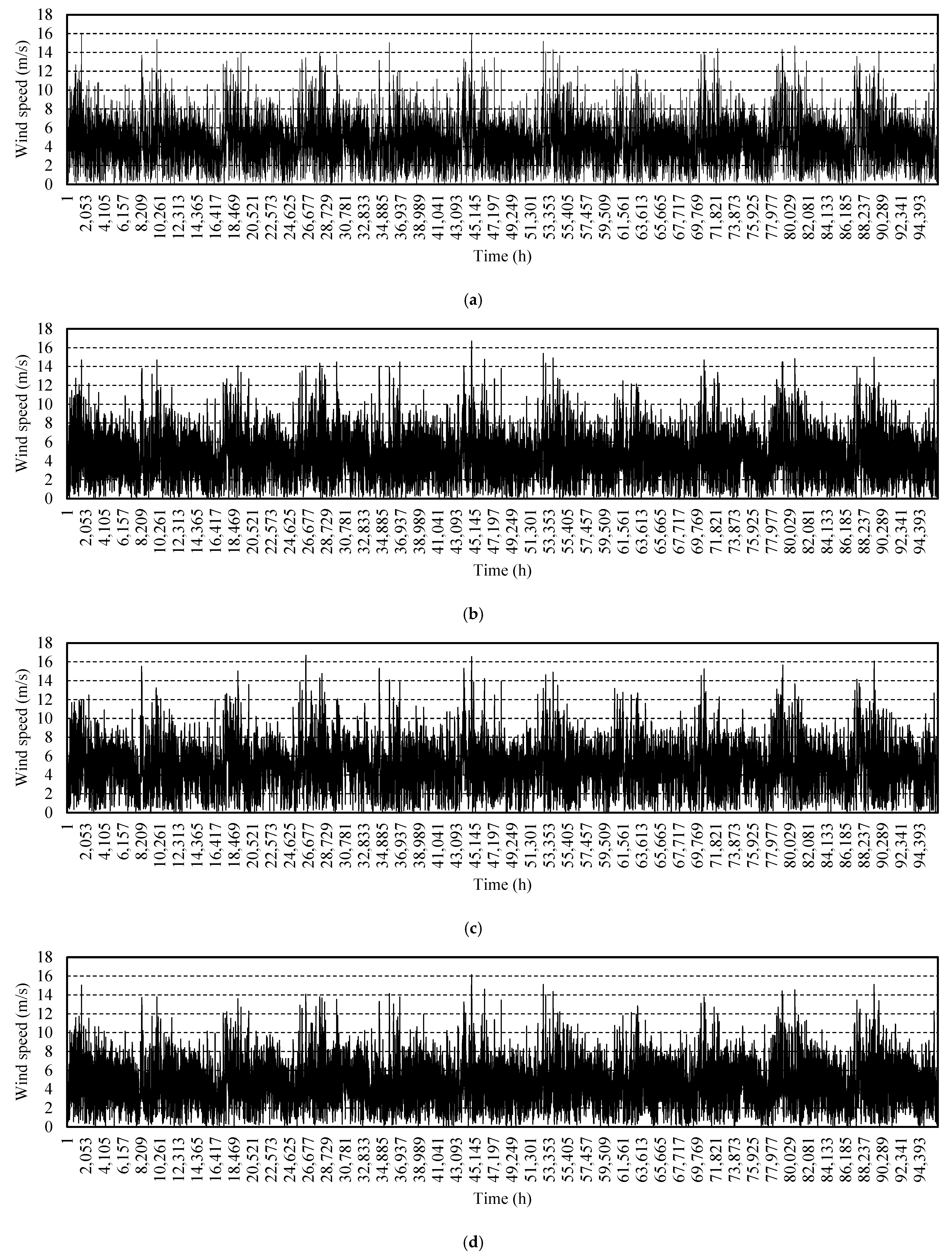
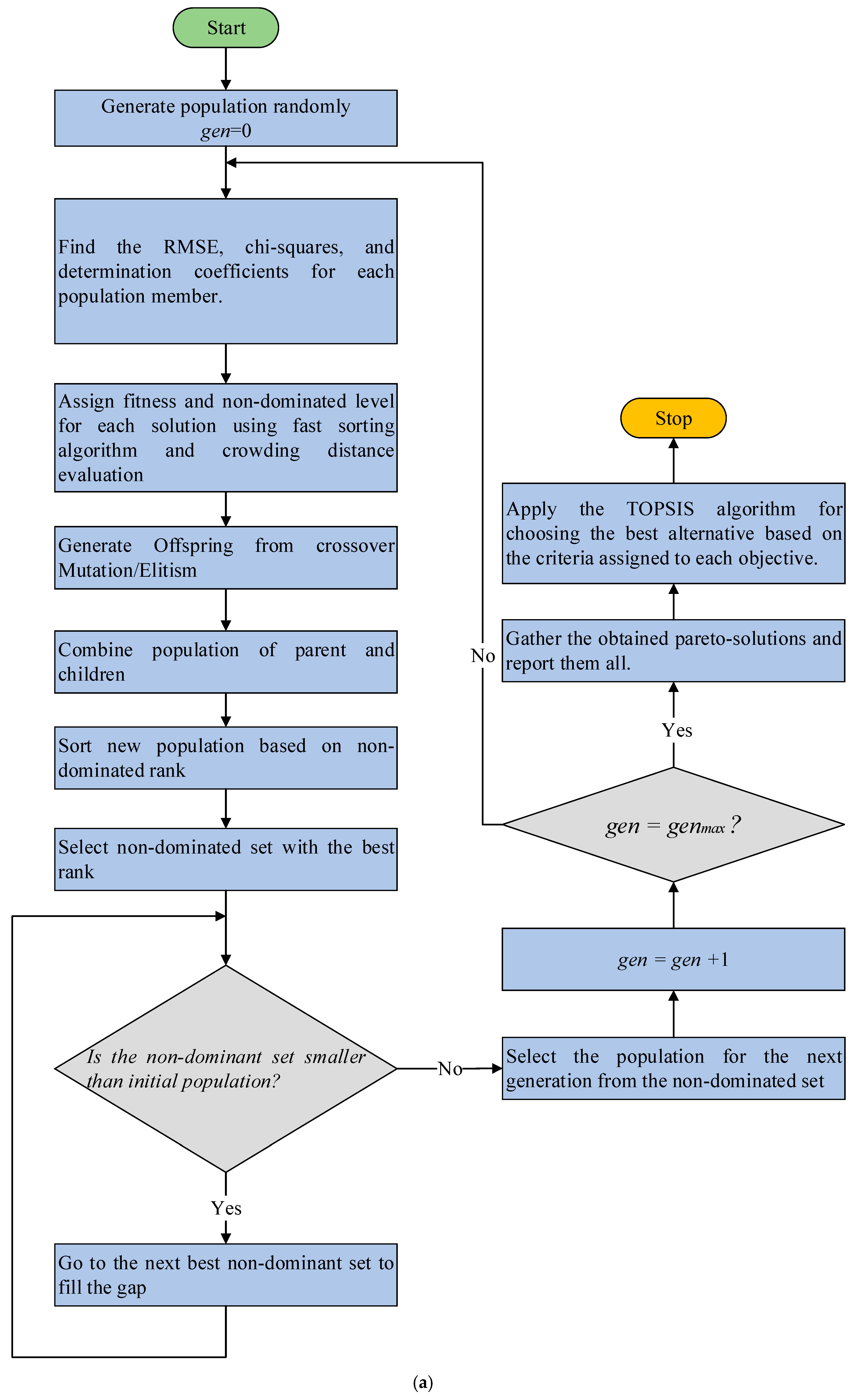
In this study, the proposed optimization algorithm was applied to fit five different sets of wind speed data extracted from various locations in Egypt [37] for 11 years, as shown in Figure 1. Two efficient multiobjective optimization algorithms were employed to solve the proposed optimization problem, namely, the nondominated sorting genetic algorithm (NSGA-II) and the multiobjective particle swarm (MOPSO). We chose these because they have been previously shown to be effective against many heuristic optimizers in solving electrical engineering applications, such as hosting capacity enhancement [10]. Both NSGA-II and MOPSO flowcharts are shown in Figure 2. The obtained pareto-front solutions were further processed via a multicriteria decision-making algorithm called “technique for order of preference by similarity to ideal solution” (TOPSIS) [38,39,40] to obtain the best solution that meets the predefined criteria ($\mathrm{\mu }$), which gives $RMSE$ a priority twice as $R^2$ and $X^2$. Thus, the $RMSE$ contributes 50% in choosing the optimum solution(s), denoted by ${\mathrm{\mu }}_1$ and equal to 0.5, whereas the contribution of $R^2$ and $X^2$ is 0.25, denoted by ${\mathrm{\mu }}_2$ and ${\mathrm{\mu }}_3$, respectively. Case studies were divided into two stages, namely, equal and variable wind speed class spacings. The variable spacings started by finding the unique values of the wind speed profile and then creating the wind speed classes based on these unique values. These case studies were conducted to optimally shape the wind profile probabilistic characteristics via combined PDFs. The number of iterations of the MOPSO and NSGA-II was 100, and the population size was set to 1000. Both algorithms were executed 10 times to obtain near-optimal pareto-front solutions. For NSGA-II, the crossover and mutation percentages were 70% and 40%, respectively, and the mutation rate was 10%. For MOPSO, the archive size was set to 50, the inertia weight was 0.4, the individual and swarm confidence factors were set to 2, and number of segments in a dimension was set to 20.

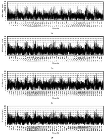
Figure 1. Wind speed data for different sites in the North Coast region of Egypt for 11 years: (a) Site 1 located in Sidi Barani, (b) Site 2 located in El-Mathany, (c) Site 3 located in Ras El-Hekma, (d) Site 4 located in El-Galaa, (e) Site 5 located in Port Said.

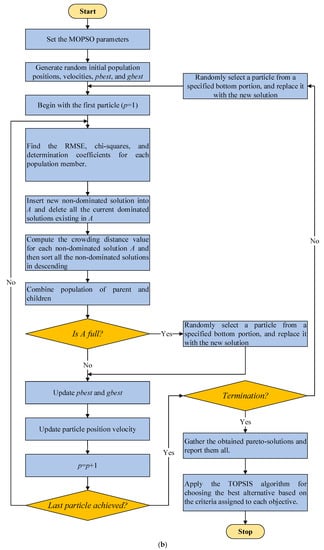
Figure 2. Flowchart of the used multiobjective optimization algorithms: (a) NSGA-II, (b) MOPSO.

3.1. Equal Wind Speed Spacings

In this case study, the NSGA-II and MOPSO are employed to solve the optimization formulation in which the obtained pareto solutions were then prioritized via the TOPSIS decision-making algorithm. The wind speed classes are characterized by its equal spacing in this case study for the obtained solutions in the five Egyptian sites. The obtained results are shown in Table 2, Table 3, Table 4, Table 5 and Table 6.

Table 2. Results obtained for 10 equal wind speed spacings in the five Egyptian sites.

Site Number	${\mathit{N}}_{\mathit{m}\mathit{i}\mathit{x}}$	NSGA-II			MOPSO
		$\mathit{R}\mathit{M}\mathit{S}\mathit{E}$	${\mathit{R}}^2$	${\mathit{X}}^2$	$\mathit{R}\mathit{M}\mathit{S}\mathit{E}$	${\mathit{R}}^2$	${\mathit{X}}^2$
1	1	0.01077	0.97666	0.00012	0.00625	0.99214	0.00004
	2	0.01237	0.96922	0.00015	0.00625	0.99214	0.00004
	3	0.01840	0.93193	0.00035	0.00540	0.99412	0.00003
2	1	0.01097	0.97548	0.00012	0.00783	0.98750	0.00006
	2	0.01182	0.97154	0.00014	0.00723	0.98933	0.00005
	3	0.02853	0.83421	0.00084	0.00113	0.99973	0.000001
3	1	0.00367	0.99687	0.000014	0.00338	0.99735	0.00001
	2	0.00703	0.98852	0.000051	0.00283	0.99815	0.00001
	3	0.01208	0.96616	0.000151	0.00192	0.99915	0.00000
4	1	0.01005	0.97987	0.000104	0.00579	0.99333	0.00003
	2	0.01552	0.95201	0.000249	0.00579	0.99332	0.00003
	3	0.01629	0.94714	0.000275	0.00579	0.99333	0.00003
5	1	0.01127	0.97703	0.000131	0.00774	0.98919	0.00006
	2	0.00850	0.98695	0.000074	0.00474	0.99594	0.00002
	3	0.01600	0.95374	0.000265	0.00777	0.98909	0.00006

Table 3. Results obtained for 20 equal wind speed spacings in the five Egyptian sites.

Site Number	${\mathit{N}}_{\mathit{m}\mathit{i}\mathit{x}}$	NSGA-II			MOPSO
		$\mathit{R}\mathit{M}\mathit{S}\mathit{E}$	${\mathit{R}}^2$	${\mathit{X}}^2$	$\mathit{R}\mathit{M}\mathit{S}\mathit{E}$	${\mathit{R}}^2$	${\mathit{X}}^2$
1	1	0.00378	0.99713	0.00003	0.00269	0.99855	0.00001
	2	0.00386	0.99700	0.00003	0.00269	0.99855	0.00001
	3	0.00910	0.98335	0.00017	0.00302	0.99816	0.00002
2	1	0.00553	0.99401	0.00006	0.00392	0.99699	0.00003
	2	0.00764	0.98860	0.00012	0.00388	0.99705	0.00003
	3	0.02006	0.92126	0.00084	0.00221	0.99904	0.00001
3	1	0.00901	0.98174	0.00017	0.00877	0.98273	0.00016
	2	0.00941	0.98012	0.00018	0.00418	0.99608	0.00004
	3	0.03002	0.79738	0.00187	0.00531	0.99366	0.00006
4	1	0.00551	0.99421	0.00006	0.00437	0.99637	0.00004
	2	0.00791	0.98810	0.00013	0.00303	0.99826	0.00002
	3	0.01302	0.96771	0.00035	0.00418	0.99668	0.00004
5	1	0.01279	0.97174	0.00051	0.00547	0.99477	0.00006
	2	0.01335	0.96923	0.00055	0.00930	0.98486	0.00018
	3	0.02308	0.90804	0.00166	0.00930	0.98486	0.00018

Table 4. Results obtained for 30 equal wind speed spacings in the five Egyptian sites.

Site Number	${\mathit{N}}_{\mathit{m}\mathit{i}\mathit{x}}$	NSGA-II			MOPSO
		$\mathit{R}\mathit{M}\mathit{S}\mathit{E}$	${\mathit{R}}^2$	${\mathit{X}}^2$	$\mathit{R}\mathit{M}\mathit{S}\mathit{E}$	${\mathit{R}}^2$	${\mathit{X}}^2$
1	1	0.00757	0.98874	0.00018	0.00583	0.99331	0.00011
	2	0.00781	0.98802	0.00019	0.00600	0.99292	0.00011
	3	0.00781	0.98802	0.00019	0.00601	0.99291	0.00011
2	1	0.00728	0.98963	0.00017	0.00693	0.99062	0.00015
	2	0.01531	0.95420	0.00073	0.00646	0.99185	0.00013
	3	0.01501	0.95599	0.00070	0.00378	0.99720	0.00004
3	1	0.00940	0.98015	0.00028	0.00888	0.98231	0.00025
	2	0.00947	0.97987	0.00028	0.00503	0.99431	0.00008
	3	0.00947	0.97987	0.00028	0.00664	0.99012	0.00014
4	1	0.00850	0.98652	0.00022	0.00705	0.99072	0.00015
	2	0.00875	0.98570	0.00024	0.00683	0.99128	0.00015
	3	0.01455	0.96047	0.00066	0.00393	0.99712	0.00005
5	1	0.01279	0.97174	0.00051	0.01085	0.97966	0.00037
	2	0.01335	0.96923	0.00055	0.01100	0.97909	0.00038
	3	0.02308	0.90804	0.00166	0.00795	0.98907	0.00020

Table 5. Weights and PDFs parameters of $f_{mix}$ for 30 equal wind speed spacings using the NSGA-II algorithm.

Site Number	${\mathit{N}}_{\mathit{m}\mathit{i}\mathit{x}}$	$\mathit{i}$	${\mathit{\omega }}_{\mathit{i},1}$	${\mathit{\omega }}_{\mathit{i},2}$	${\mathit{\omega }}_{\mathit{i},3}$	${\mathit{\omega }}_{\mathit{i},4}$	${\mathit{k}}_{\mathit{i},1}$	${\mathit{c}}_{\mathit{i},1}$	${\mathit{k}}_{\mathit{i},2}$	${\mathit{c}}_{\mathit{i},2}$	${\mathit{k}}_{\mathit{i},3}$	${\mathit{c}}_{\mathit{i},4}$
1	1	1	0.00034	0.99454	0.00476	0.00036	73.79385	31.70703	4.58715	0.00000	0.14127	68.98417
	2	1	0.00000	0.46317	0.00000	0.15381	40.35879	52.73686	4.55628	32.28912	53.80212	3.08534
		2	0.00000	0.38181	0.00120	0.00000	27.25824	68.94476	4.87313	10.49539	29.27796	37.76996
	3	1	0.00363	0.00000	0.01140	0.00000	53.24860	17.27855	53.58056	29.09172	82.68204	79.97628
		2	0.01046	0.59690	0.00000	0.30576	85.03399	18.89028	4.55835	57.89836	95.61217	3.18172
		3	0.00339	0.00000	0.00305	0.06542	74.13813	80.12175	67.48028	59.15287	77.12520	4.14649
2	1	1	0.00000	0.93619	0.00001	0.06380	42.29673	40.00127	4.67366	47.89578	63.84122	2.93954
	2	1	0.00312	0.29239	0.00312	0.27655	59.85635	67.81208	5.08736	90.33011	31.44685	3.85625
		2	0.00074	0.00439	0.00122	0.41848	14.39543	87.70615	29.67952	51.12360	31.67918	3.09742
	3	1	0.00000	0.06065	0.00000	0.23550	58.39489	80.55814	5.86088	27.32205	23.62730	3.25214
		2	0.04392	0.22702	0.00204	0.20465	70.97043	50.58780	4.83515	44.31630	13.10943	2.78105
		3	0.00036	0.20202	0.01206	0.01180	42.98833	97.77294	4.77987	48.23871	10.40638	73.34310
3	1	1	0.00008	0.79294	0.00006	0.20692	62.46275	47.86930	5.45810	42.67871	72.18348	3.29967
	2	1	0.00059	0.37752	0.00000	0.00029	48.52595	33.06928	5.26438	48.55042	27.14744	64.93494
		2	0.03049	0.34396	0.00079	0.24636	6.37485	18.59843	5.40582	57.45784	32.64139	3.75803
	3	1	0.03058	0.31613	0.00000	0.01436	86.74505	16.95936	5.30614	110.02295	109.94055	53.50350
		2	0.00438	0.00784	0.02601	0.02267	40.87161	25.94324	59.53822	55.79216	74.74296	66.49486
		3	0.00000	0.34241	0.00589	0.22974	48.01248	70.81428	5.09028	42.42671	37.93132	3.33625
4	1	1	0.00000	0.99196	0.00000	0.00804	50.39877	38.65348	4.54251	57.70120	64.43584	0.51050
	2	1	0.00082	0.55058	0.00111	0.00002	58.22308	54.34909	4.52033	68.20038	42.90745	44.47037
		2	0.00001	0.44574	0.00098	0.00074	65.74181	42.79643	4.57082	39.46333	49.92005	41.76769
	3	1	0.01843	0.37132	0.00711	0.00711	100.80900	23.27993	4.68969	5.21841	24.45806	63.15324
		2	0.00000	0.00897	0.00000	0.25849	93.43002	55.97088	38.23371	80.30763	16.09118	2.91898
		3	0.00109	0.27949	0.03128	0.01670	85.56484	69.20576	4.62985	26.15153	20.36618	73.51160
5	1	1	0.00000	1.00000	0.00000	0.00000	93.58844	62.72201	4.52723	91.81758	31.06219	55.05638
	2	1	0.00220	0.00000	0.00000	0.23560	38.40924	80.26567	63.15395	41.28379	91.10511	3.17433
		2	0.00085	0.56303	0.00278	0.19554	54.54940	90.12121	4.68333	92.85935	94.94080	3.44225
	3	1	0.03576	0.14250	0.00158	0.14397	4.44326	20.08993	4.87683	62.12001	78.51489	3.38791
		2	0.01290	0.01042	0.02693	0.13176	42.83066	20.97307	55.61803	12.77200	105.65023	3.62303
		3	0.02093	0.19415	0.06682	0.21228	92.34193	76.29295	4.27876	61.69388	71.89037	2.84531

Table 6. Weights and PDFs parameters of $f_{mix}$ for 30 equal wind speed spacings using the MOPSO algorithm.

Site Number	${\mathit{N}}_{\mathit{m}\mathit{i}\mathit{x}}$	$\mathit{i}$	${\mathit{\omega }}_{\mathit{i},1}$	${\mathit{\omega }}_{\mathit{i},2}$	${\mathit{\omega }}_{\mathit{i},3}$	${\mathit{\omega }}_{\mathit{i},4}$	${\mathit{k}}_{\mathit{i},1}$	${\mathit{c}}_{\mathit{i},1}$	${\mathit{k}}_{\mathit{i},2}$	${\mathit{c}}_{\mathit{i},2}$	${\mathit{k}}_{\mathit{i},3}$	${\mathit{c}}_{\mathit{i},4}$
1	1	1	0.01821	0.96666	0.00000	0.01513	3.37535	15.02806	4.65127	86.33833	89.92111	0.73477
	2	1	0.00120	0.91121	0.00366	0.06386	94.49952	34.89852	4.67373	39.70831	5.23394	3.13871
		2	0.00364	0.01498	0.00022	0.00122	3.44163	98.89050	1.35853	98.27957	92.78617	95.40006
	3	1	0.00454	0.39526	0.00035	0.17120	57.49185	29.55937	4.70232	53.42064	28.91840	3.07179
		2	0.00267	0.00007	0.00014	0.00000	98.60259	0.05260	87.46580	7.99455	47.69958	3.84613
		3	0.00364	0.42077	0.00069	0.00069	3.39093	86.53919	4.76569	92.12256	18.34722	76.94156
2	1	1	0.00022	0.99152	0.00000	0.00827	3.56125	90.62619	4.63615	32.34890	100.00000	0.60339
	2	1	0.00004	0.44466	0.00001	0.00059	61.93793	11.45986	4.75095	93.26458	35.38043	0.68524
		2	0.00433	0.44259	0.00001	0.10778	3.61378	93.54713	4.75204	56.47268	10.98078	2.89341
	3	1	0.00276	0.67577	0.00033	0.00016	5.73793	100.00000	4.91475	77.00172	95.07571	98.29700
		2	0.00303	0.00139	0.00004	0.18126	5.15555	85.17888	48.63691	6.94460	25.38179	3.17867
		3	0.06753	0.00618	0.00024	0.06130	3.54492	6.70900	70.40451	9.44477	92.23108	3.18446
3	1	1	0.00000	0.96999	0.00000	0.03001	85.84468	73.37492	5.31757	94.37597	24.62790	0.93811
	2	1	0.00021	0.37095	0.00000	0.00051	93.96757	91.55658	5.68172	53.04907	89.84384	95.68243
		2	0.26747	0.00016	0.00287	0.35783	5.47647	3.80692	85.08386	0.06256	0.18635	3.55755
	3	1	0.00348	0.00044	0.00044	0.00000	5.63902	98.36905	5.10485	97.94978	99.77773	1.49898
		2	0.00469	0.95568	0.00012	0.00000	5.16733	97.94739	5.31828	54.66384	33.97096	1.67987
		3	0.00000	0.00008	0.00004	0.03502	88.65839	99.35837	61.42782	70.84273	19.28514	0.96339
4	1	1	0.05474	0.93121	0.00000	0.01405	3.44476	5.69593	4.67193	13.14709	74.36018	0.69841
	2	1	0.00259	0.00000	0.00001	0.00001	2.91999	93.67475	85.95537	67.18377	90.97950	3.07029
		2	0.00000	0.98644	0.00000	0.01096	28.21660	1.16557	4.60459	72.68700	99.30794	0.59264
	3	1	0.03486	0.25170	0.00027	0.22097	3.81408	13.67664	4.77332	96.86787	98.86956	3.06168
		2	0.00526	0.23869	0.00000	0.00019	4.94044	85.60790	4.91013	1.59959	98.42046	81.38206
		3	0.01927	0.22188	0.00676	0.00014	2.87242	19.75791	4.77571	40.28597	48.74096	99.75578
5	1	1	0.00398	0.86969	0.00968	0.11665	5.31591	100.00000	4.60534	0.00000	0.33532	2.90385
	2	1	0.00407	0.97775	0.00000	0.01818	5.31612	100.00000	4.52537	8.12529	77.09078	0.70752
		2	0.00000	0.00000	0.00000	0.00000	84.42821	75.58742	48.06149	88.04431	12.17536	75.14713
	3	1	0.39641	0.39505	0.00024	0.00030	5.19388	3.23347	4.37112	40.45326	36.80202	60.87665
		2	0.00001	0.00038	0.00019	0.18097	52.34119	45.15843	78.13708	5.86943	3.34522	2.65902
		3	0.00045	0.00001	0.00016	0.02584	96.82498	2.58698	94.49701	70.61560	91.64219	2.78155

As shown by the results given in Table 2, Table 3 and Table 4 the proposed optimization strategy succeeded in finding the best fit using NSGA-II or MOPSO. The MOPSO achieved better results than NSGA-II for different numbers of $N_{mix}$. For instance, for Site 1, as shown in Table 4, the $RMSE$ values using MOPSO were 0.00583, 0.006, and 0.00601, for $N_{mix}$ of 1, 2, and 3, respectively, which were better than the $RMSE$ values of 0.00757, 0.00781, and 0.00781 obtained using NSGA-II. The MOPSO obtained better $R^2$ values of 0.01548, 0.02292, and 0.06219, for $N_{mix}$ of 1, 2, and 3, respectively, which were greater than the values obtained using NSGA-II. Finally, the MOPSO obtained better $X^2$ values of 0.00008, 0.00011, and 0.00032, for $N_{mix}$ of 1, 2, and 3, respectively, which were greater than the values obtained using NSGA-II.

3.2. Variable Wind Speed Spacings

In this case study, the wind speed classes were characterized by their variable spacing for the obtained solutions in the five Egyptian sites. The obtained results are shown in Table 7, Table 8 and Table 9.

Table 7. Results obtained for variable wind speed spacings in the five Egyptian sites.

Site Number	${\mathit{N}}_{\mathit{m}\mathit{i}\mathit{x}}$	NSGA-II			MOPSO
		$\mathit{R}\mathit{M}\mathit{S}\mathit{E}$	${\mathit{R}}^2$	${\mathit{X}}^2$	$\mathit{R}\mathit{M}\mathit{S}\mathit{E}$	${\mathit{R}}^2$	${\mathit{X}}^2$
1	1	0.00788	0.98786	0.00141	0.00951	0.98232	0.00205
	2	0.00819	0.98690	0.00152	0.00682	0.99090	0.00106
	3	0.01706	0.94310	0.00660	0.00718	0.98994	0.00117
2	1	0.00777	0.98847	0.00139	0.00722	0.99006	0.00120
	2	0.00769	0.98871	0.00137	0.00639	0.99221	0.00094
	3	0.00717	0.99018	0.00119	0.00722	0.99006	0.00120
3	1	0.00996	0.97804	0.00239	0.00605	0.99191	0.00088
	2	0.01115	0.97246	0.00300	0.00612	0.99171	0.00090
	3	0.01496	0.95046	0.00539	0.00864	0.98347	0.00180
4	1	0.00803	0.98821	0.00145	0.00604	0.99332	0.00082
	2	0.00733	0.99017	0.00121	0.01978	0.92842	0.00879
	3	0.00722	0.99047	0.00117	0.00804	0.98818	0.00145
5	1	0.01137	0.97784	0.00273	0.00686	0.99193	0.00099
	2	0.01137	0.97783	0.00273	0.01168	0.97661	0.00288
	3	0.01140	0.97771	0.00274	0.00704	0.99151	0.00105

Table 8. Weights and PDFs parameters of $f_{mix}$ for variable wind speed spacings using the NSGA-II algorithm.

Site Number	${\mathit{N}}_{\mathit{m}\mathit{i}\mathit{x}}$	$\mathit{i}$	${\mathit{\omega }}_{\mathit{i},1}$	${\mathit{\omega }}_{\mathit{i},2}$	${\mathit{\omega }}_{\mathit{i},3}$	${\mathit{\omega }}_{\mathit{i},4}$	${\mathit{k}}_{\mathit{i},1}$	${\mathit{c}}_{\mathit{i},1}$	${\mathit{k}}_{\mathit{i},2}$	${\mathit{c}}_{\mathit{i},2}$	${\mathit{k}}_{\mathit{i},3}$	${\mathit{c}}_{\mathit{i},4}$
1	1	1	0.0002	0.8444	0.0000	0.1554	48.425	44.339	4.669	41.365	56.543	3.020
	2	1	0.0017	0.6721	0.0025	0.0021	6.149	63.774	4.726	33.273	45.119	71.640
		2	0.0003	0.3188	0.0020	0.0005	43.398	49.205	4.234	18.297	46.592	39.919
	3	1	0.00000	0.14944	0.06649	0.20311	55.683	30.748	4.510	63.154	97.451	3.653
		2	0.01027	0.00187	0.01447	0.22116	60.377	35.709	78.467	57.418	53.484	3.377
		3	0.00495	0.20368	0.00000	0.12456	42.480	68.215	4.903	73.196	22.711	3.414
2	1	1	0.00000	1.00000	0.00000	0.00000	54.213	48.625	4.582	27.172	44.266	41.026
	2	1	0.00002	0.91132	0.00003	0.08856	49.728	44.948	4.678	35.551	49.427	2.750
		2	0.00000	0.00003	0.00003	0.00001	75.194	48.409	14.680	4.062	40.727	10.036
	3	1	0.07615	0.37523	0.00010	0.00024	4.363	3.110	4.616	10.767	64.974	25.395
		2	0.00024	0.48102	0.00036	0.05832	98.824	22.681	4.705	19.240	78.937	2.999
		3	0.00006	0.00026	0.00026	0.00778	23.999	33.205	25.256	18.865	68.288	0.444
3	1	1	0.00000	0.95662	0.04337	0.00000	69.044	63.562	5.233	0.000	0.825	46.606
	2	1	0.00000	0.99528	0.00000	0.00000	50.286	5.686	5.222	67.739	26.628	50.970
		2	0.00022	0.00101	0.00155	0.00194	37.671	38.236	48.929	65.213	33.951	35.914
	3	1	0.01790	0.10200	0.01711	0.16985	84.899	62.419	5.231	30.359	81.995	3.771
		2	0.00509	0.24629	0.00000	0.19175	60.529	64.694	5.039	46.647	65.495	3.643
		3	0.00835	0.21782	0.00653	0.01731	83.843	36.780	5.329	24.729	45.280	59.468
4	1	1	0.00000	0.98961	0.00000	0.01039	55.636	53.742	4.524	85.219	42.310	0.481
	2	1	0.00002	0.98496	0.00003	0.00980	48.350	39.747	4.514	14.155	26.492	0.487
		2	0.00516	0.00001	0.00001	0.00003	3.634	87.108	57.749	63.339	16.895	37.124
	3	1	0.02622	0.11545	0.00000	0.08101	6.792	13.172	5.370	98.985	73.486	4.193
		2	0.20249	0.23195	0.00144	0.11972	3.780	4.559	4.324	91.330	0.110	4.321
		3	0.05869	0.00130	0.00027	0.16147	5.664	9.177	81.345	8.644	80.996	2.809
5	1	1	0.00000	0.76647	0.00000	0.23353	53.558	75.748	4.661	39.797	37.620	2.931
	2	1	0.00000	0.41577	0.00000	0.23707	40.008	60.686	4.690	59.175	91.911	2.936
		2	0.00000	0.34716	0.00000	0.00000	50.291	53.204	4.634	43.035	42.309	30.106
	3	1	0.00001	0.18816	0.00000	0.00002	55.752	58.751	4.618	58.510	58.645	72.007
		2	0.00002	0.26503	0.00001	0.24116	56.536	64.118	4.581	31.815	46.300	2.964
		3	0.00000	0.30557	0.00000	0.00002	49.509	39.171	4.760	37.036	15.008	48.917

Table 9. Weights and PDFs parameters of $f_{mix}$ for variable wind speed spacings using the MOPSO algorithm.

Site Number	${\mathit{N}}_{\mathit{m}\mathit{i}\mathit{x}}$	$\mathit{i}$	${\mathit{\omega }}_{\mathit{i},1}$	${\mathit{\omega }}_{\mathit{i},2}$	${\mathit{\omega }}_{\mathit{i},3}$	${\mathit{\omega }}_{\mathit{i},4}$	${\mathit{k}}_{\mathit{i},1}$	${\mathit{c}}_{\mathit{i},1}$	${\mathit{k}}_{\mathit{i},2}$	${\mathit{c}}_{\mathit{i},2}$	${\mathit{k}}_{\mathit{i},3}$	${\mathit{c}}_{\mathit{i},4}$
1	1	1	0.71401	0.00000	0.00000	0.28599	4.55643	2.57959	97.38555	87.80310	26.76532	4.45092
	2	1	0.00051	0.75905	0.00480	0.21317	100.00000	78.93519	4.79506	93.09646	37.09961	3.01302
		2	0.02103	0.00107	0.00023	0.00014	3.145	9.304	96.366	0.429	39.610	98.845
	3	1	0.31049	0.00003	0.00030	0.00059	4.56479	2.22783	95.71619	95.62623	0.82070	100.00000
		2	0.00003	0.33572	0.00001	0.00018	72.563	81.813	4.641	70.750	39.824	49.771
		3	0.00515	0.34737	0.00013	0.00000	2.955	83.338	4.782	99.382	78.309	62.951
2	1	1	0.00000	0.98877	0.00000	0.01123	42.49486	99.11726	4.58684	40.24957	98.33208	0.49573
	2	1	0.00005	0.95083	0.01507	0.00379	93.86458	67.05292	4.67894	0.01003	0.73239	0.53725
		2	0.02964	0.00058	0.00001	0.00004	3.317	7.608	1.157	0.000	96.174	78.740
	3	1	0.00000	0.33870	0.00000	0.00000	95.85218	88.92973	4.59392	84.23408	90.74424	97.69710
		2	0.00000	0.33216	0.00000	0.00000	95.340	30.944	4.587	0.657	86.978	96.636
		3	0.00000	0.31786	0.00000	0.01127	57.419	93.756	4.580	66.668	45.022	0.497
3	1	1	0.28131	0.66437	0.00000	0.05432	5.44750	3.55836	5.30209	81.05400	58.40800	1.18226
	2	1	0.00004	0.00017	0.00006	0.01955	94.82906	5.07351	7.34059	26.43792	29.42188	3.67992
		2	0.18047	0.75892	0.00004	0.04074	5.648	4.297	5.163	86.680	69.339	0.982
	3	1	0.00001	0.35346	0.00000	0.00000	95.82083	94.46366	5.24176	34.60687	71.87913	7.45724
		2	0.00536	0.24103	0.00002	0.03192	4.944	96.758	5.263	47.223	1.018	0.865
		3	0.00000	0.36815	0.00001	0.00002	45.800	34.308	5.274	9.265	93.706	76.604
4	1	1	0.04979	0.93428	0.00000	0.01593	3.38081	6.42380	4.62992	16.16983	42.17319	0.60484
	2	1	0.00000	0.00000	0.00000	1.00000	81.75708	39.00862	100.00000	99.99985	23.80490	3.43200
		2	0.00000	0.00000	0.00000	0.00000	97.990	58.772	99.779	99.828	81.813	53.125
	3	1	0.00039	0.00000	0.00050	0.00065	47.15409	0.52431	97.70312	99.66505	3.66957	99.97253
		2	0.00532	0.00000	0.00066	0.00142	3.583	47.404	99.897	98.599	4.632	99.815
		3	0.00100	0.96516	0.00023	0.02466	70.379	16.386	4.553	4.757	87.988	2.746
5	1	1	0.38471	0.59667	0.00000	0.01863	5.15268	3.30579	4.07631	24.63107	7.26524	0.56759
	2	1	0.00000	0.97334	0.00000	0.00000	96.03999	18.92268	4.53098	3.58419	36.69862	36.10664
		2	0.00000	0.02666	0.00000	0.00000	98.882	76.903	1.421	91.753	98.591	0.561
	3	1	0.32427	0.00021	0.00015	0.00000	5.18747	3.43628	97.42475	18.64058	9.66750	10.81575
		2	0.00012	0.23193	0.00017	0.00550	48.676	60.676	4.321	29.575	54.779	0.416
		3	0.00000	0.22487	0.00000	0.21279	93.373	99.473	4.342	99.654	90.231	2.804

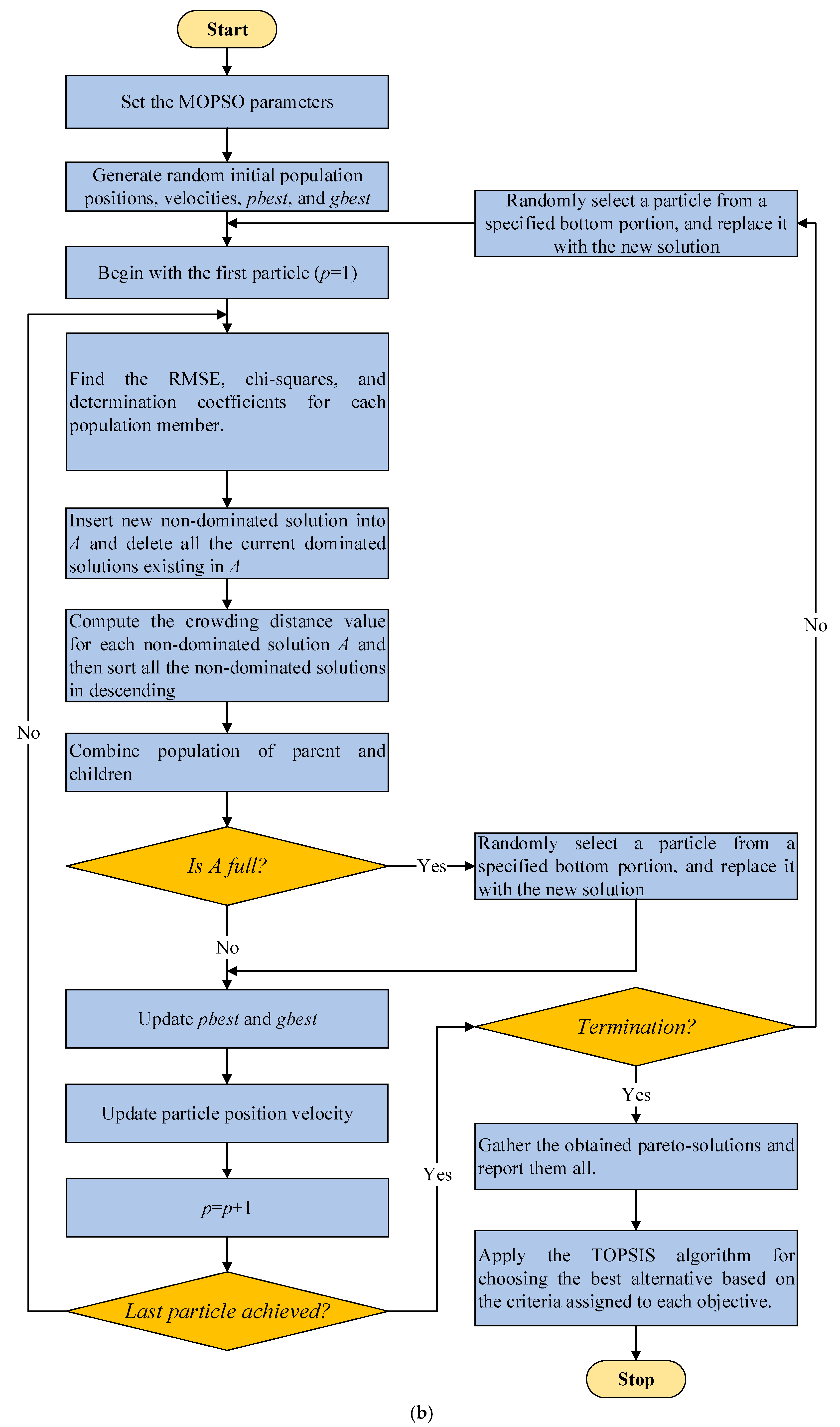
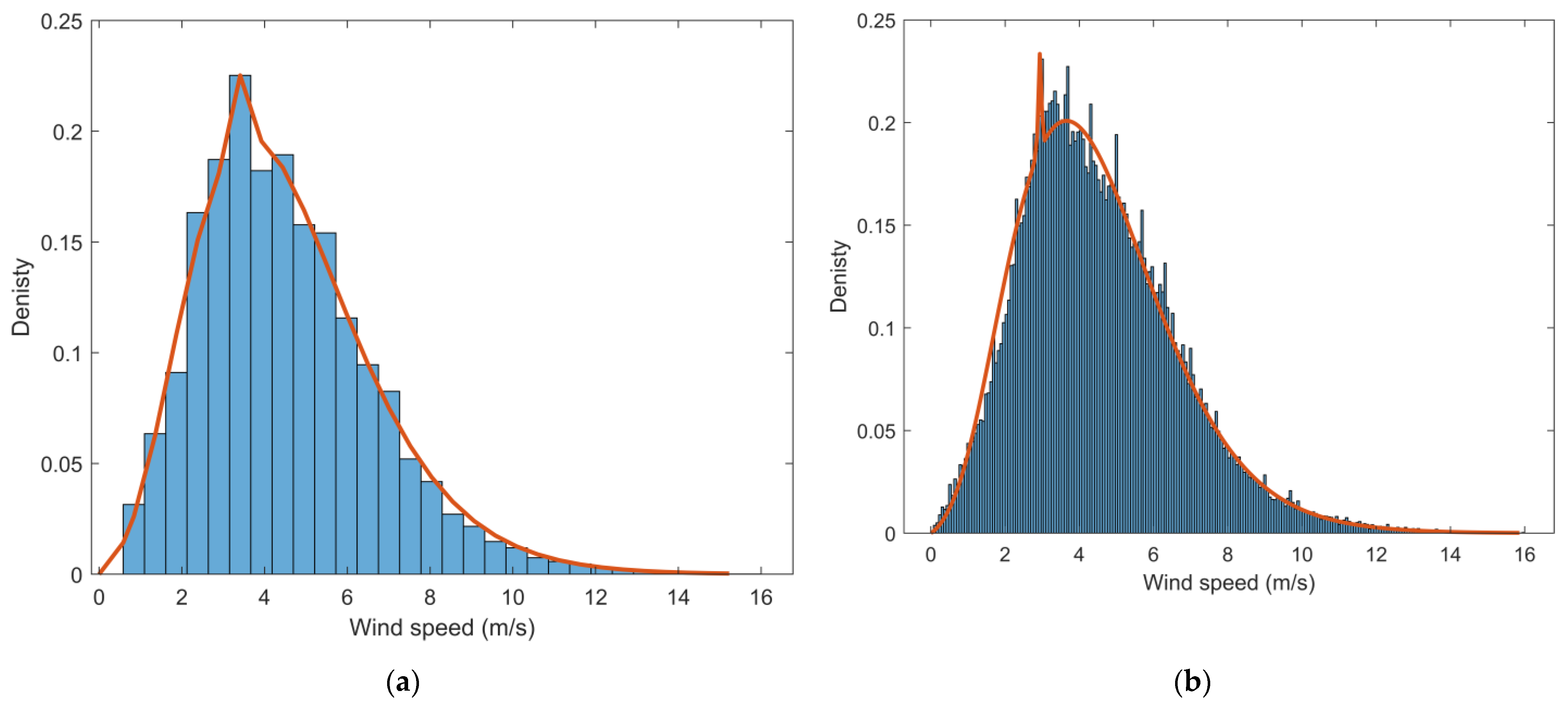
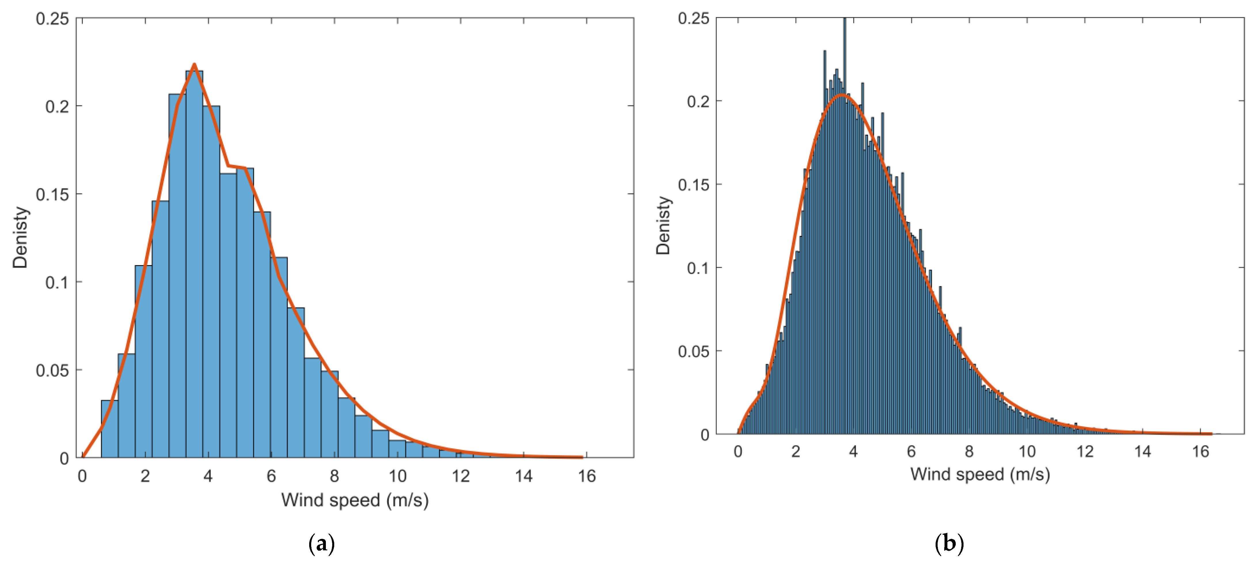
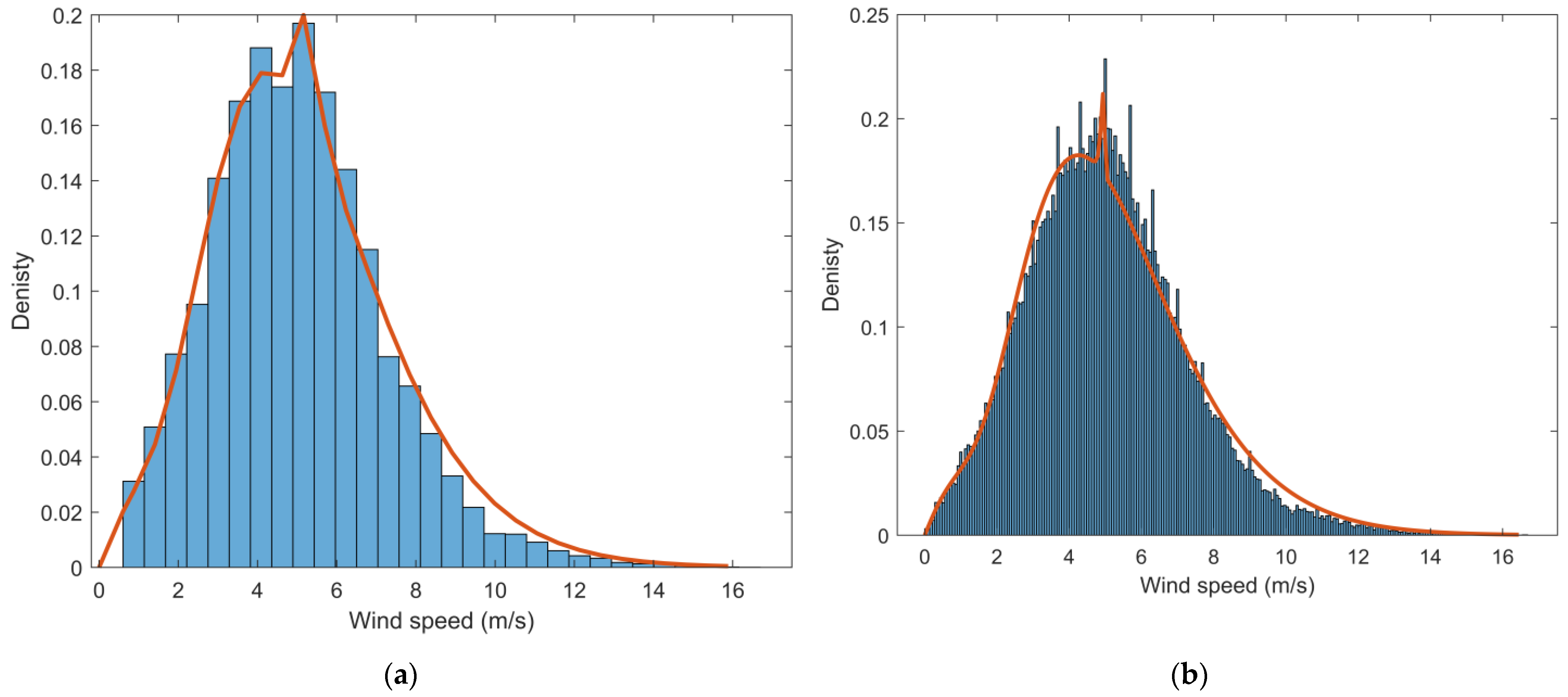
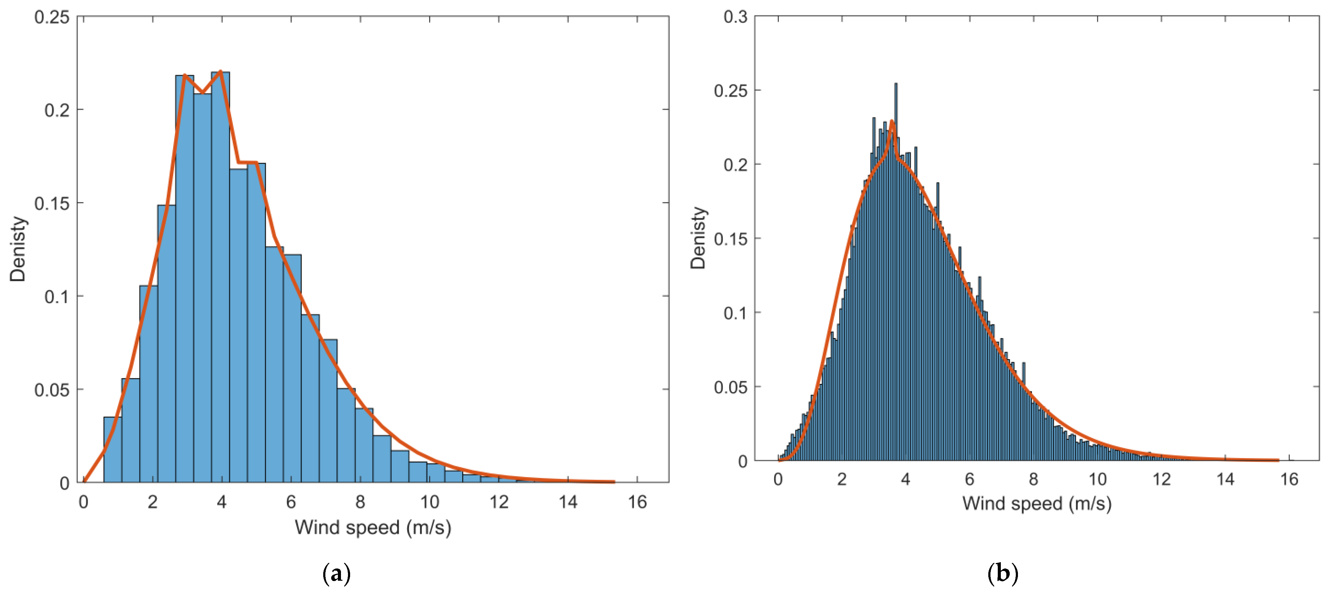
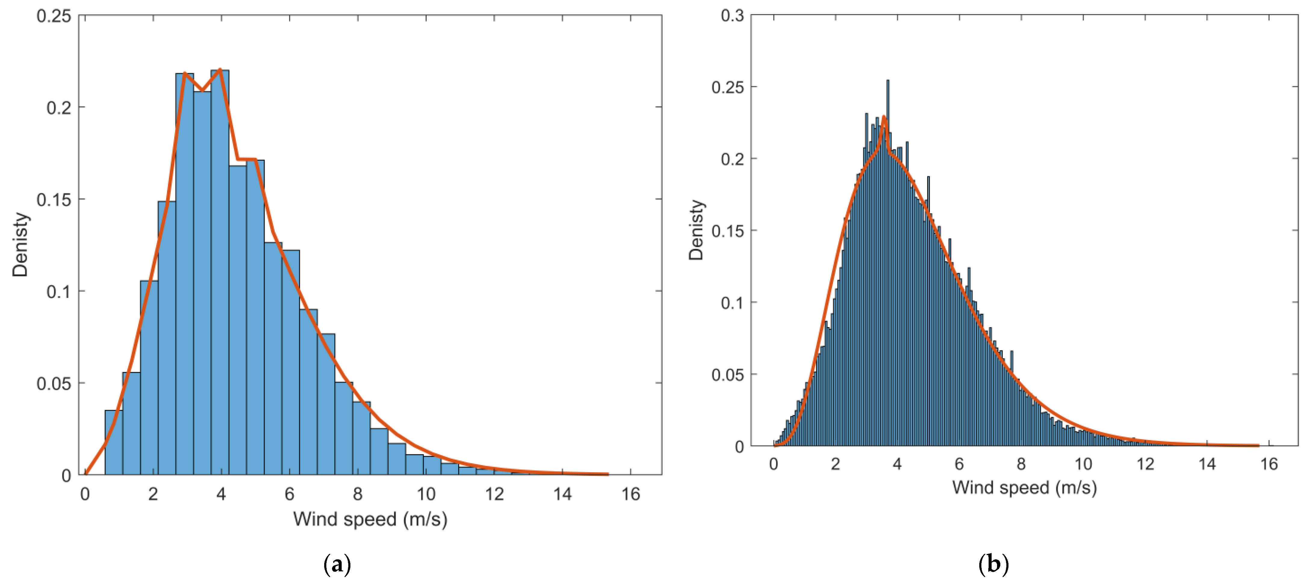
From the obtained results, we concluded that the variable speed classes provided a more realistic shape for the probabilistic nature of the wind speed profiles from different viewpoints. First, from the obtained shape viewpoint, the approximate PDFs obtained using 10, 20, and 30 wind speed classes, shown in Figure 3, Figure 4, Figure 5, Figure 6 and Figure 7 provided a limited shape for the wind speed profile compared to using the variable speed profile, where all the wind speeds included in the wind speed profile were taken into consideration and thus provided near-accurate values for the probability of each wind speed. Second, the nonlinearity of the shape of the wind speed profile, as shown in Figure 3, Figure 4, Figure 5, Figure 6 and Figure 7, was advantageous for the variable wind speed classes compared to the equal ones, although the equal wind speed classes might give better $RMSE$ or $R^2$ or $X^2$ values using MOPSO. Moreover, from the obtained results, it can be noted that there was no need for some PDFs to shape the wind speed profile to the given data, where its obtained weights (${\omega }_{i,j}, j\in \left\{1,2,3,4\right\}$) was equal to zero. Further, from the optimization viewpoint, the MOPSO succeeded in providing $RMSE$, $R^2$, and $X^2$ values that were better than those obtained using NSGA-II in many cases, such as in Site 1 in the case of variable wind speed profile, as shown in Table 7. However, we could not judge which optimizer was better as NSGA-II sometimes gave better values than MOPSO. For instance, as shown in Table 7, in Site 1, the $RMSE$ using NSGA-II was 0.00163 lower than that using MOPSO, and the $R^2$ using NSGA-II was 0.00554 greater than MOPSO for $N_{mix}$ of 1. However, in Site 1, the $RMSE$ was 0.00137 lower using MOPSO than using NSGA-II, and the $R^2$ using MOPSO was 0.004 greater than NSGA-II for $N_{mix}$ of 2. Thus, unlike in the equal class width case study illustrated in Section 3.1, it is difficult to recommend one optimizer for the variable class width.

Figure 3. Fitting wind data of Site 1 to $f_{mix}$ using MOPSO: (a) 30 equal wind speed spacings; (b) variable wind speed spacings.

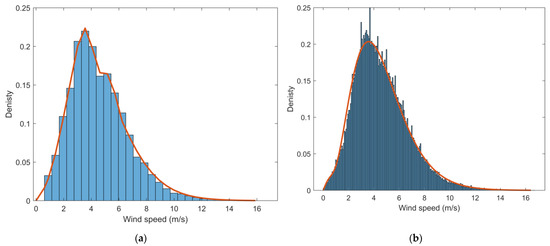
Figure 4. Fitting wind data of Site 2 to $f_{mix}$ using MOPSO: (a) 30 equal wind speed spacings; (b) variable wind speed spacings.

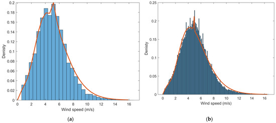
Figure 5. Fitting wind data of Site 3 to $f_{mix}$ using MOPSO: (a) 30 equal wind speed spacings; (b) variable wind speed spacings.

Figure 6. Fitting wind data of Site 4 to $f_{mix}$ using MOPSO: (a) 30 equal wind speed spacings; (b) variable wind speed spacings.

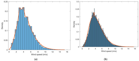
Figure 7. Fitting wind data of Site 5 to $f_{mix}$ using MOPSO: (a) 30 equal wind speed spacings; (b) variable wind speed spacings.

3.3. Comparison of NSGA-II and MOPSO

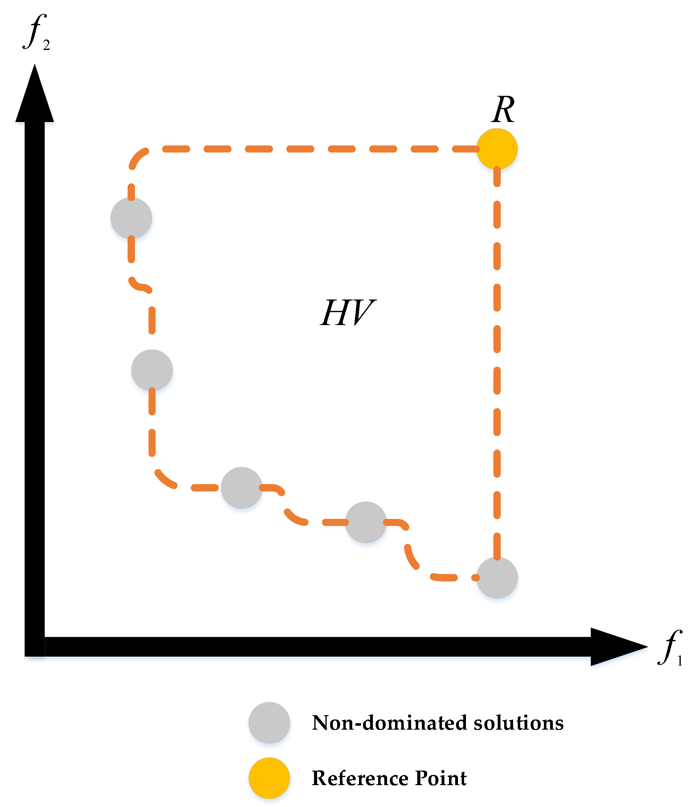
From the obtained results, we needed to confirm that the results would vary for the tested optimizers. Various methodologies have previously been presented to compare multiobjective optimization techniques, such as hyper volume index, the spacing metric, and others [41,42,43,44,45]. In this work, the hyper volume ($HV$) index [41,42,43] was employed to compare the obtained pareto-fronts from NSGA-II and MOPSO. The higher the $HV$ value, the more near-optimal the pareto-front obtained. The formulation of the $HV$ index is expressed in Equation (7).

$$HV\left(B_k,R\right)=volume({{\displaystyle \cup }}_{i=1}^{\left|B_k\right|}{v}_i)$$

(7)

where the set of pareto-solutions for the kth optimizer is denoted by $B_k$, and the reference point is denoted by $R$, where $R$ is set to the maximum value of the pareto-solutions ($R=\max \left\{B_1, B_2, \dots \right\}$). The hypercube ($v$) comprises corners, including both $R$ and $B_k$, as shown in Figure 8, for a multiobjective example composed of two objectives $f_1$ and $f_2$.

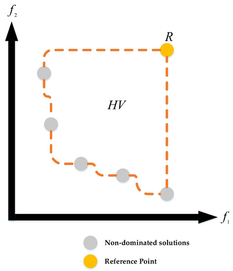
Figure 8. Hyper volume enclosed by nondominated solutions and the reference point.

Table 10 illustrates the obtained $HV$ values for the variable and equal wind speed spacing case studies. For Site 1, the NSGA-II showed superiority over MOPSO as the $HV$ was a higher value, which ensured the closeness of its pareto-solutions to the optimal pareto-solution for the variable case study. For Site 2, the MOPSO showed superiority over NSGA-II for the variable case study. For Site 1, the NSGA-II had a near-optimal pareto-front that was better than MOPSO for 30 equal wind speed spacings. Thus, we can confirm that the pareto-solutions of heuristic optimizers will vary, and we cannot recommend a particular optimizer.

Table 10. Comparison between NSGA-II and MOPSO using the hyper volume index.

Case Study	Variable Wind Speed Spacings		Thirty Equal Wind Speed Spacings
Site	NSGA-II	MOPSO	NSGA-II	MOPSO
1	0.3014	0.2949	0.2900	0.2870
2	0.2484	0.2553	0.2886	0.3000
3	0.2920	0.2972	0.2713	0.2834
4	0.3060	0.2973	0.3050	0.3127
5	0.3019	0.2786	0.2657	0.2837

4. Conclusions

In this work, a novel mixture probability composed of four well-known probability density functions was designed to obtain better results for wind speed profiles for different case studies, including equal and variable spacings. The MOPSO succeeded in finding a near-optimal solution for the equal spacing case study, and the result was better than that obtained using NSGA-II for different number of spacings and for different sites. The variable spacing case study provided a new realistic insight to the probability of wind speed included in the wind speed data, and the obtained mixture PDF was much better than fixing the number of wind speed classes. Moreover, the variable case study showed the difficulty in recommending a particular optimizer. A comparison between the pareto-fronts of NSGA-II and MOPSO was conducted to clarify that none of the optimizers was better than the other. In future, the authors will use the results from this research to model the wind speed profile of wind turbines supplying electricity to real microgrids and analyze the obtained indices to maximize the power injected to different loads. In addition, we will analyze the effect of inserting wind turbines on controlling various energy systems, such as islanded systems [46,47,48,49].

References

- Cruz, M.R.M.; Fitiwi, D.Z.; Santos, S.F.; Catalão, J.P.S. A comprehensive survey of flexibility options for supporting the low-carbon energy future. Renew. Sustain. Energy Rev. 2018, 97, 338–353. [Google Scholar] [CrossRef]
- Muradov, N.; Veziroglu, T. “Green” path from fossil-based to hydrogen economy: An overview of carbon-neutral technologies. Int. J. Hydrogen Energy 2008, 33, 6804–6839. [Google Scholar] [CrossRef]
- Hanley, E.S.; Deane, J.; Gallachóir, B.Ó. The role of hydrogen in low carbon energy futures–A review of existing perspectives. Renew. Sustain. Energy Rev. 2018, 82, 3027–3045. [Google Scholar] [CrossRef]
- Fan, L.; Tu, Z.; Chan, S.H. Recent development of hydrogen and fuel cell technologies: A review. Energy Rep. 2021, 7, 8421–8446. [Google Scholar] [CrossRef]
- Mostafa, M.H.; Aleem, S.H.E.A.; Ali, S.G.; Abdelaziz, A.Y.; Ribeiro, P.F.; Ali, Z.M. Robust Energy Management and Economic Analysis of Microgrids Considering Different Battery Characteristics. IEEE Access 2020, 8, 54751–54775. [Google Scholar] [CrossRef]
- Mostafa, M.H.; Abdel Aleem, S.H.E.; Ali, S.G.; Ali, Z.M.; Abdelaziz, A.Y. Techno-economic assessment of energy storage systems using annualized life cycle cost of storage (LCCOS) and levelized cost of energy (LCOE) metrics. J. Energy Storage 2020, 29, 101345. [Google Scholar] [CrossRef]
- Abdel Aleem, S.H.E.; Zobaa, A.F.; Balci, M.E.; Ismael, S.M. Harmonic Overloading Minimization of Frequency-Dependent Components in Harmonics Polluted Distribution Systems Using Harris Hawks Optimization Algorithm. IEEE Access 2019, 7, 100824–100837. [Google Scholar] [CrossRef]
- Diaaeldin, I.M.; Abdel Aleem, S.H.E.; El-Rafei, A.; Abdelaziz, A.Y.; Zobaa, A.F. Hosting capacity maximization based on optimal reconfiguration of distribution networks with optimized soft open point operation. In Hosting Capacity for Smart Power Grids; Springer: Berlin/Heidelberg, Germany, 2020; ISBN 9783030400293. [Google Scholar]
- Diaaeldin, I.M.; Abdel Aleem, S.H.E.; El-Rafei, A.; Abdelaziz, A.Y.; Zobaa, A.F. Large-scale integration of distributed generation in reconfigured distribution networks considering load uncertainty. In Uncertainties in Modern Power Systems; Elsevier: Amsterdam, The Netherlands, 2021; pp. 441–484. [Google Scholar]
- Ali, Z.M.; Diaaeldin, I.M.; Abdel Aleem, S.H.E.; El-Rafei, A.; Abdelaziz, A.Y.; Jurado, F. Scenario-based network reconfiguration and renewable energy resources integration in large-scale distribution systems considering parameters uncertainty. Mathematics 2021, 9, 26. [Google Scholar] [CrossRef]
- Ismael, S.; Abdel Aleem, S.; Abdelaziz, A.; Zobaa, A. Probabilistic Hosting Capacity Enhancement in Non-Sinusoidal Power Distribution Systems Using a Hybrid PSOGSA Optimization Algorithm. Energies 2019, 12, 1018. [Google Scholar] [CrossRef]
- El-Fergany, A.A.; Abdelaziz, A.Y. Capacitor allocations in radial distribution networks using cuckoo search algorithm. IET Gener. Transm. Distrib. 2014, 8, 223–232. [Google Scholar] [CrossRef]
- Ali, Z.M.; Diaaeldin, I.M.; El-Rafei, A.; Hasanien, H.M.; Abdel Aleem, S.H.E.; Abdelaziz, A.Y. A novel distributed generation planning algorithm via graphically-based network reconfiguration and soft open points placement using Archimedes optimization algorithm. Ain Shams Eng. J. 2021, 12, 1923–1941. [Google Scholar] [CrossRef]
- Ismael, S.M.; Abdel Aleem, S.H.E.; Abdelaziz, A.Y.; Zobaa, A.F. State-of-the-art of hosting capacity in modern power systems with distributed generation. Renew. Energy 2019, 130, 1002–1020. [Google Scholar] [CrossRef]
- Khamees, A.K.; Abdelaziz, A.Y.; Eskaros, M.R.; Attia, M.A. Investigation of Different Probability Distribution Functions for Wind Speed Modelling Using Classical and Novel Metaheuristic Methods. In Proceedings of the 2021 22nd International Middle East Power Systems Conference (MEPCON), Assiut, Egypt, 14–16 December 2021; pp. 26–31. [Google Scholar]
- Akdağ, S.A.; Bagiorgas, H.S.; Mihalakakou, G. Use of two-component Weibull mixtures in the analysis of wind speed in the Eastern Mediterranean. Appl. Energy 2010, 87, 2566–2573. [Google Scholar] [CrossRef]
- Pishgar-Komleh, S.H.; Keyhani, A.; Sefeedpari, P. Wind speed and power density analysis based on Weibull and Rayleigh distributions (a case study: Firouzkooh county of Iran). Renew. Sustain. Energy Rev. 2015, 42, 313–322. [Google Scholar] [CrossRef]
- Baran, S.; Lerch, S. Log-normal distribution based Ensemble Model Output Statistics models for probabilistic wind-speed forecasting. Q. J. R. Meteorol. Soc. 2015, 141, 2289–2299. [Google Scholar] [CrossRef]
- Khamees, A.K.; Abdelaziz, A.Y.; Eskaros, M.R.; Attia, M.A.; Badr, A.O. The Mixture of Probability Distribution Functions for Wind and Photovoltaic Power Systems Using a Metaheuristic Method. Processes 2022, 10, 2446. [Google Scholar] [CrossRef]
- Van der Auwera, L.; de Meyer, F.; Malet, L. The use of the Weibull three-parameter model for estimating mean wind power densities. J. Appl. Meteorol. Climatol. 1980, 19, 819–825. [Google Scholar] [CrossRef]
- Carta, J.A.; Ramírez, P. Use of finite mixture distribution models in the analysis of wind energy in the Canarian Archipelago. Energy Convers. Manag. 2007, 48, 281–291. [Google Scholar] [CrossRef]
- Celik, A.N. Energy output estimation for small-scale wind power generators using Weibull-representative wind data. J. Wind. Eng. Ind. Aerodyn. 2003, 91, 693–707. [Google Scholar] [CrossRef]
- Khamees, A.K.; Abdelaziz, A.Y.; Ali, Z.M.; Alharthi, M.M.; Ghoneim, S.S.; Eskaros, M.R.; Attia, M.A. Mixture probability distribution functions using novel metaheuristic method in wind speed modeling. Ain Shams Eng. J. 2022, 13, 101613. [Google Scholar] [CrossRef]
- Brano, V.L.; Orioli, A.; Ciulla, G.; Culotta, S. Quality of wind speed fitting distributions for the urban area of Palermo, Italy. Renew. Energy 2011, 36, 1026–1039. [Google Scholar] [CrossRef]
- Labeeuw, W.; Deconinck, G. Customer sampling in a smart grid pilot. In Proceedings of the 2012 IEEE Power and Energy Society General Meeting, San Diego, CA, USA, 22–26 July 2012; IEEE: Piscataway, NJ, USA, 2012. [Google Scholar]
- Salameh, Z.M.; Borowy, B.S.; Amin, A.R. Photovoltaic module-site matching based on the capacity factors. IEEE Trans. Energy Convers. 1995, 10, 326–332. [Google Scholar] [CrossRef]
- Shi, G.; Eftekharnejad, S. Impact of solar forecasting on power system planning. In Proceedings of the 2016 North American Power Symposium (NAPS), Denver, CO, USA, 18–20 September 2016; IEEE: Piscataway, NJ, USA, 2016. [Google Scholar]
- Tizgui, I.; El Guezar, F.; Bouzahir, H.; Benaid, B. Comparison of methods in estimating Weibull parameters for wind energy applications. Int. J. Energy Sect. Manag. 2017, 11, 650–663. [Google Scholar] [CrossRef]
- Kang, D.; Ko, K.; Huh, J. Comparative study of different methods for estimating Weibull parameters: A case study on Jeju Island, South Korea. Energies 2018, 11, 356. [Google Scholar] [CrossRef]
- Suwarno, I.Y.; Irwanto, M.; Hiendro, A. Analysis of wind speed characteristics using different distribution models in Medan City, Indonesia. Int. J. Power Electron. Drive Syst. 2021, 12, 1102. [Google Scholar] [CrossRef]
- Zhao, X.; Wang, C.; Su, J.; Wang, J. Research and application based on the swarm intelligence algorithm and artificial intelligence for wind farm decision system. Renew. Energy 2019, 134, 681–697. [Google Scholar] [CrossRef]
- Saeed, M.A.; Ahmed, Z.; Yang, J.; Zhang, W. An optimal approach of wind power assessment using Chebyshev metric for determining the Weibull distribution parameters. Sustain. Energy Technol. Assess. 2020, 37, 100612. [Google Scholar] [CrossRef]
- Guedes, K.S.; de Andrade, C.F.; Rocha, P.A.; Mangueira, R.D.S.; de Moura, E.P. Performance analysis of metaheuristic optimization algorithms in estimating the parameters of several wind speed distributions. Appl. Energy 2020, 268, 114952. [Google Scholar] [CrossRef]
- Coello Coello, C.A.; Lechuga, M.S. MOPSO: A proposal for multiple objective particle swarm optimization. In Proceedings of the 2002 Congress on Evolutionary Computation. CEC’02 (Cat. No.02TH8600), Honolulu, HI, USA, 12–17 May 2002; IEEE: New York, NY, USA, 2002; Volume 2, pp. 1051–1056. [Google Scholar]
- Deb, K.; Pratap, A.; Agarwal, S.; Meyarivan, T. A fast and elitist multiobjective genetic algorithm: NSGA-II. IEEE Trans. Evol. Comput. 2002, 6, 182–197. [Google Scholar] [CrossRef]
- Omar, O.A.M.; Ahmed, H.M.; Elbarkouky, R.A. Commercial wind turbines modeling using single and composite cumulative probability density functions. Int. J. Electr. Comput. Eng. (IJECE) 2021, 11, 47. [Google Scholar] [CrossRef]
- Global Wind Atlas. Available online: https://globalwindatlas.info/en (accessed on 11 February 2023).
- Hwang, C.-L.; Yoon, K. Multiple Attributes Decision Making Methods and Applications. 1981. Available online: https://www.springer.com/gp/book/9783540105589 (accessed on 11 February 2023).
- Yoon, K. A Reconciliation among Discrete Compromise Solutions. J. Oper. Res. Soc. 1987, 38, 277. [Google Scholar] [CrossRef]
- Hwang, C.-L.; Lai, Y.-J.; Liu, T.-Y. A new approach for multiple objective decision making. Comput. Oper. Res. 1993, 20, 889–899. [Google Scholar] [CrossRef]
- Ahmadi, B.; Ceylan, O.; Ozdemir, A. Reinforcement of the distribution grids to improve the hosting capacity of distributed generation: Multi-objective framework. Electr. Power Syst. Res. 2023, 217, 109120. [Google Scholar] [CrossRef]
- Ahmadi, B.; Ceylan, O.; Ozdemir, A.; Fotuhi-Firuzabad, M. A multi-objective framework for distributed energy resources planning and storage management. Appl. Energy 2022, 314, 118887. [Google Scholar] [CrossRef]
- Fleischer, M. The measure of Pareto optima applications to multi-objective metaheuristics. Lect. Notes Comput. Sci. 2003, 2632, 519–533. [Google Scholar] [CrossRef]
- Tao, S.; Xu, Q.; Feijoo, A.; Zheng, G. Joint Optimization of Wind Turbine Micrositing and Cabling in an Offshore Wind Farm. IEEE Trans. Smart Grid 2021, 12, 834–844. [Google Scholar] [CrossRef]
- yang, J.; Zheng, S.; Song, D.; Su, M.; Yang, X.; Joo, Y.H. Comprehensive Optimization for Fatigue Loads of Wind Turbines in Complex-Terrain Wind Farms. IEEE Trans. Sustain. Energy 2021, 12, 909–919. [Google Scholar] [CrossRef]
- Zhang, N.; Sun, Q.; Yang, L.; Li, Y. Event-Triggered Distributed Hybrid Control Scheme for the Integrated Energy System. IEEE Trans. Ind. Inform. 2022, 18, 835–846. [Google Scholar] [CrossRef]
- Yang, L.; Li, X.; Sun, M.; Sun, C. Hybrid Policy-based Reinforcement Learning of Adaptive Energy Management for the Energy Transmission-constrained Island Group. IEEE Trans. Ind. Inform. 2023, 1–12. [Google Scholar] [CrossRef]
- Omar, O.A.M.; Ahmed, H.M.; Elbarkouky, R.A. Wind turbines new criteria optimal site matching under new capacity factor probabilistic approaches. Energy Syst. 2021, 2021, 1–26. [Google Scholar] [CrossRef]
- Afifi, M.A.; Marei, M.I.; Mohamad, A.M.I. Modelling, Analysis and Performance of a Low Inertia AC-DC Microgrid. Appl. Sci. 2023, 13, 3197. [Google Scholar] [CrossRef]
Disclaimer/Publisher’s Note: The statements, opinions and data contained in all publications are solely those of the individual author(s) and contributor(s) and not of MDPI and/or the editor(s). MDPI and/or the editor(s) disclaim responsibility for any injury to people or property resulting from any ideas, methods, instructions or products referred to in the content. |
© 2023 by the authors. Licensee MDPI, Basel, Switzerland. This article is an open access article distributed under the terms and conditions of the Creative Commons Attribution (CC BY) license (https://creativecommons.org/licenses/by/4.0/).