Analysis of a Queuing System with Possibility of Waiting Customers Jockeying between Two Groups of Servers

Abstract

In this paper, we consider a queueing system consisting of two multi-server subsystems that is designed for the service of clients arriving at a system according to a Markovian arrival process (MAP). Arriving clients receive information about the number of clients present in both subsystems and use this information to make a randomized decision to balk (depart without receiving service) or join the system. In the latter case, they also decide which subsystem they would like to join. One subsystem has an infinite buffer, while the buffer of the second subsystem is finite. The service time distribution is exponential in the first subsystem and phase-type in the second subsystem. During the waiting in the chosen buffers, after the random time intervals, each waiting client checks the status of the alternative subsystem. If some server in that subsystem is idle during this epoch, the client immediately leaves the buffer where it has been staying and starts a service in the alternative subsystem. The problem of computing the steady-state distribution of this system is solved. The feasibility of the proposed solution and certain features of the system’s behavior are numerically illustrated.

1. Introduction

Due to limited resources, waiting in queues is an inevitable feature of human life. When a person arrives for service at some system and cannot start receiving the service immediately, he/she has to decide whether to wait until the service device is available or depart from the system without service. In the former case, a common situation is that there are several service devices, and the person has to decide which queue he/she will join. The problem of choosing the proper queue can be difficult. Most often, the choice of the person (below, we call him/her the client) is based on the comparison of the lengths of the queues to the servers. However, due to the random duration of the service process for clients, the reasonable choice to join the shortest queue may not guarantee the minimal waiting time. After a client joins some queue, it may occur that a certain alternative queue decreases more quickly. In real-world systems, this may lead to the so-called jockeying of the clients from one queue to another currently shorter one. The main purpose of the queueing theory is to build and analyze adequate models of real systems to optimally (in terms of some revenue criterion) manage their operations. Thus, the jockeying phenomenon has already attracted a lot of attention in the queuing literature. Note that the models with jockeying are similar to models in which clients have to choose among several queues and do this according to the shortest queue rule; see, e.g., [1]. For references to the literature relating to the models with jockeying, see, for example, papers [2,3,4,5,6,7,8,9,10,11,12].

In the early paper [2], the models with two single-server devices, two stationary Poisson arrival processes, and an exponential distribution of service times are considered. Three different strategies for client scheduling are considered. One of them suggests initially joining the shortest queue. Further, a client can jump to the alternative queue if that one becomes shorter. More general and popular in the literature, the jockeying rule assumes that the jump occurs when the difference between the lengths of queues exceeds a fixed threshold. Such a type of model was analyzed, e.g., in [7]. Systems with more than two servers are dealt with in [3,4,5,6]. The majority of papers assume that the buffers are infinite. In [10], a model with two servers and finite buffers was under study.

The overwhelming majority of existing papers suggest that the arrival flows are defined by the stationary Poisson arrival process. However, this suggestion is not realistic in many modern real-world systems. In the paper [4], the renewal arrival process is supposed, i.e., inter-arrival times are independent and identically arbitrarily distributed. This allows modelling real-world systems more adequately because not only the average arrival rate but also higher moments of the distribution of inter-arrival times, including their variance, can be taken into account. In the paper [8], the asymptotic behavior for the $MAP/PH/c$ queue with the shortest queue discipline and jockeying is analyzed. Here, $PH$ denotes the phase-type distribution of service times, and $MAP$ denotes the Markovian arrival process. This process, initially introduced by M. Neuts as a versatile arrival process, allows taking into account not only the mean value and variance of inter-arrival times but also the correlation of these times. This makes the $MAP$ a good model of modern arrival processes in telecommunication networks, contact centers, etc. More useful information about the $MAP$ can be found, e.g., in [13,14,15,16,17,18,19,20,21].

In our paper, we also assume that clients arrive according to the $MAP.$ Supplementary to [8], where the author presented only an approximate analysis of the tail decay rate of the stationary distribution of the longest queue, here we present an exact algorithmic analysis of the whole queuing system. The considered model of jockeying is different from the one suggested in [8] and other models considered in the existing literature.

Our model is formulated based on the authors’ personal experience of visiting supermarkets, airports, and various offices. For example, we will briefly describe a real-life scenario in which it can be applied to the terminology of supermarkets.

In modern supermarkets, often the bottleneck is the area of payment for the products after their selection by clients. Usually, there are two zones for consumers to checkout in supermarkets. Service in one zone is provided by several independent human cashiers. The second zone consists of several independent self-service devices (SSDs) specially designed for clients’ self-service. The popularity and usefulness of the wide use of SSDs are mentioned in many papers; for reference, see, e.g., [22]. Usually, the two zones mentioned are located close to each other but are more or less spatially divided. Thus, there are separate queues for customers waiting for service in these zones.

The arriving client observes the lengths of both queues and makes decisions based on his/her own preferences, experience, psychology, the importance of shopping right now in this supermarket, etc. One possible decision is to immediately depart (balk) from the system without service. Such a decision, as a rule, is taken if the consumer evaluates that the required waiting time exceeds the value appropriate for him/her, he/she does not have a discount card for this supermarket, and there are alternative supermarkets in the vicinity. Another decision is to join the system. In this case, the client has to make one more decision: to join the queue in the zone with cashiers or the queue for SSDs. We assume that both decisions are randomized, with the probabilities depending on the length of the queues and the personality of the client. Statistics about typical values of such probabilities may be available, at least for supermarket managers, in modern, highly computerized supermarkets equipped with video surveillance systems.

After joining some queue, the client should wait until he/she is picked up for the service from this queue according to the First In–First Out discipline. In the majority of queuing models with clients jockeying, it is supposed that the tagged client permanently monitors the length of all queues. The client jockeys to another queue if he/she sees that the difference between the length of the queue in front of him/her and some alternative queue reaches some fixed value in the advance threshold. Multiple reverse jockeying is usually possible. This may be a realistic scenario in some real-world systems.

In our model (with two multi-server service devices), we analyze another realistic scenario that we usually observe in real supermarkets. First of all, when making decisions about the preferred queues, clients may not use the standard rule considered in many research papers: to join the shortest queue. This is because the prospective waiting time depends not only on the queue length but also on the number of servers and the rate of their operation. Another reason for making a choice in another way may be the a priori preference of the customer. Some users may prefer to receive service at SSDs due to various reasons related to psychology or knowledge of the language. Another user prefers human cashiers due to a lack of or negative experience with operating with SSDs.

After joining a queue, clients in supermarkets usually do not permanently keep track of both queue lengths, and, as it was just said, they are not very informative. Consumers may prefer not to continuously monitor the queue and use spare time to call by phone or browse the Internet. We assume that the clients staying in the queue can watch the state of the alternative queuing system after the random time intervals. We assume that the client, observing that the alternative system has an idle server, leaves his/her place in the current queue, moves to another zone, and immediately starts service there.

Thus, we suggest that each client not jockey between queues several times. He/she may jockey only once and only when he/she has an opportunity to immediately start service in the alternative queue. It is worth noting that the analyzed scenario of jockeying is: (i) realistic in supermarket modeling; (ii) a bit similar to the mechanism of customer retrials in a multi-server queue with repeated attempts and the classical strategy of retrials. For references to the literature devoted to the analysis of retrial queues; see, e.g., [23,24,25]. Clients staying in some queue of the system under study behave similarly to customers staying in the orbit of the respective retrial multi-server queue.

The discipline of jockeying used in our model allows the system to be more conservative, i.e., to reduce the possibility of some servers staying idle when there are waiting clients, on the one hand. On the other hand, it allows the avoidance of chaos that can occur when many clients frequently jockey between the queues under the traditional threshold jockeying discipline.

As has already been mentioned, although we gave the verbal description of the considered queueing model in terms of a supermarket, it can be formulated in terms of various other service systems. We can mention, e.g., systems for check-in, luggage drop, passport control, and security control in airports and other transport hubs, service systems in different bank, tax, and other municipal or governmental offices with the possibility of self-service, and various other real-world objects that split the common flow of requests between various groups of servers and are tolerant of users jockeying.

Because the dynamics of the queue with jockeying clients is described by at least two components (number of customers in two or more corresponding systems), it is natural that many of the papers cited above exploit the useful tool of level-independent Quasi-Birth-and-Death processes for analysis. This tool, developed mainly by M. Neuts, see, e.g., [14], leads to the computation of the stationary distribution in a quite simple matrix-geometric form. In [6], the use of so-called $GI/M/1$-type Markov allowed obtaining the solution in a similar matrix-geometric form for the system with the renewal arrival process. In our paper, due to the use of the briefly described alternative mechanism of jockeying, the behavior of the system is described by the level-dependent Quasi-Birth-and-Death process, and results from [26,27,28] are used for the computation of the stationary distribution of a multi-dimensional Markov chain describing the behavior of the considered system.

It is worth noting also that due to the assumption that the service time distribution in the SSD servers has not an exponential but a more general phase-type ($PH$) distribution, the size of the blocks in the generator of a Markov chain can be large. To make them as small as possible, we use the results obtained as the refinement of the known approach by D. Lucantoni and V. Ramaswami, see, e.g., [29,30], for constructing the Markov chain. Motivation for our consideration of $PH$-type distribution of service time in System 2 instead of a much more simple exponential distribution is the following. The model under study supplements the model of operation of SSDs in supermarkets or other systems with the possibility of self-service, which was analyzed in [22]. In [22], only the work of the system with SSDs was considered. The existence of an alternative to receiving service via cashiers was not considered. Here, we take into account this alternative. A positive feature of the model considered in [22] was the consideration of the possibility of interruptions in service by SSDs due to the occurrence of problems in service. These problems can be solved with the help of assistants. Therefore, the full service time for a client may consist of several phases of service and waiting for help. Thus, it is a good choice to model the service time by SSDs in our model, which does not directly account for the possibility of breaks, by the phase-type distribution.

In the next section, we present a mathematical model of the considered system.

2. Mathematical Model

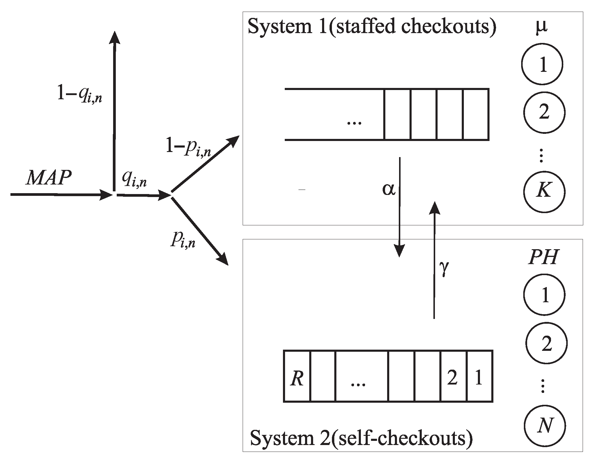
We consider a queueing model consisting of two dependent systems. System 1 consists of K servers (staffed or human checkouts) and an infinite buffer. System 2 has N servers (self-checkouts or SSDs) and a finite buffer of capacity $R$. The structure of the system under study is presented in Figure 1.

Clients arrive in the system in accordance with the $MAP$ arrival flow. This flow is defined by an underlying Markov chain ($MC$) ${\nu }_t$ with finite state space $\{1,2,\cdots ,W\}.$ Each transition of the underlying process may lead to the arrival of a client. The intensities of these chain transitions are defined by two matrices, $D_0$ and $D_1.$ The diagonal entries of matrix $D_0$ give, up to the sign, the intensities of $MC$ leaving the corresponding state. The non-diagonal entries of the matrix $D_0$ represent the intensities of $MC$ transitions that are not accompanied by the arrival of a client, while matrix $D_1$ consists of the intensities of the transitions with client arrivals. Much more information about the $MAP$ and its performance indicators can be found, e.g., in [13,14,15,16,17,18,19,20,21]. In this paper, we denote as $\lambda$ the average arrival intensity of clients in the $MAP$. This intensity can be found as $\lambda =\mathit{\theta }{D}_1\mathbf{e},$ where $\mathit{\theta }$ defines the stationary distribution of the $MAP$ and is defined as the solution to the system $\mathit{\theta }(D_0+D_1)=\mathbf{0},\mathit{\theta }\mathbf{e}=1.$ Here, $\mathbf{e}$ is a column vector of the form $(1,1,\cdots ,1)$ and $\mathbf{0}$ is a row vector of the form $(0,0,\cdots ,0)$.

We assume that each arriving client may observe the number of clients in both systems. Based on this information, the client decides whether to balk or join one of the buffers. We assume that an arriving client decides to balk with the probability $1-q_{i,n},$ where $i,i\ge 0,$ is the current number of clients in System 1 and $n,n=\overline{0,N+R},$ is the current number of clients in System 2. With the complimentary probability $q_{i,n}$, the client decides to receive service. If the client decides to receive service, he/she joins System 2 with the probability $p_{i,n}$ and arrives at System 1 with the complimentary probability. Here, we assume $p_{i,N+R}=0,$ i.e., if the finite buffer is full, the client always joins the infinite buffer.

The service time of a client in System 1 has an exponential distribution with the parameter $\mu .$ The service time distribution of a client in System 2 is of $PH$-type with an irreducible representation $(\mathit{\beta },S)$ and underlying process $m_t,t\ge 0,$ with finite state space of transient states $\{1,2,\cdots ,M\}.$ The vector $\mathit{\beta }$ defines the probability of choosing the initial state of the underlying process $m_t$ at the moment of service beginning. The sub-generator S gives the transition intensities of the $MC$ $m_t$ within the set $\{1,2,\cdots ,M\}.$ The column-vector ${\mathbf{S}}_0=-S\mathbf{e}$ defines the intensities of transition to the absorbing state. Such a transition leads to the service completion. For more information about $PH,$ the interested reader is referred to [14,19].

We assume that each client staying in the buffer of System 1 makes attempts to obtain service in System 2 without waiting with the intensity $\alpha ,\alpha >0$. The attempt is successful if, during the attempt epoch, there is at least one free server in System 2. In this case, the client leaves System 1 and starts service in System 2. If the attempt is unsuccessful, the client remains in the same place in the buffer of System 1. Analogously, the clients staying in a buffer in System 2 can make attempts to obtain service in System 1 without waiting with the intensity $\gamma$. The attempt is also assumed to be successful only if, during the attempt epoch, there is at least one free server in System 1.

Our goals are to analyze the stationary behavior of this system and give some insights into its quantitative behavior.

3. The Process of System States

The behavior of the system under consideration can be described by the following regular irreducible $MC$ with continuous time

$${\xi }_t=\{i_t,n_t,{\nu }_t,m_t^{\left(1\right)},m_t^{\left(2\right)},\cdots ,m_t^{\left(M\right)}\},t\ge 0,$$

where at time $t,t\ge 0,$

• $i_t$ is the number of clients in System 1, $i_t\ge 0;$
• $n_t$ is the number of clients in System 2, $n_t=\overline{0,N+R};$
• ${\nu }_t$ is the state of the underlying process of the $MAP$, ${\nu }_t=\overline{1,W};$
• $m_t^{\left(l\right)}$ is the number of servers at phase l of service in System 2, $l=\overline{1,M},$ $m_t^{\left(l\right)}=\overline{0,\min \{n_t,N\}},$ ${\displaystyle \sum _{l=1}^M}{m}_t^{\left(l\right)}=\min \{n_t,N\}.$

Note that, following the approach suggested in [29,30], here we monitor the numbers of servers at various phases of service in System 2 instead of keeping track of the phase of service at each busy server. This allows to essentially reduce the state space of the $MC$ describing the behavior of the system, especially when the number of servers N is large in comparison to the number of phases $M.$ The number of possible states of the components ${\mathbf{m}}_t=\{m_t^{\left(1\right)},m_t^{\left(2\right)},\cdots ,m_t^{\left(M\right)}\}$ is equal to $\frac{(N+M-1)!}{N!(M-1)!}$ under the description of service processes chosen here instead of $M^N.$ When $M=2$ and $N=20,$ the corresponding numbers are 21 and 1,048,576, respectively, see [31]. This clearly motivates our choice of the $MC.$

To analyze the $MC$ ${\xi }_t,t\ge 0,$ we enumerate its states in the direct lexicographic order of the components $\{i_t,n_t,{\nu }_t\}$ and the reverse lexicographic order of the components ${\mathbf{m}}_t.$ We will call all states of the chain that have the value i of the denumerable component $i_t$ as level i of the $MC$ ${\xi }_t.$

Let us denote the infinitesimal generator of this chain as $Q.$ The matrix Q contains intensities of all possible transitions of the considered chain during an infinitesimally short time interval.

Theorem 1.

The infinitesimal generator Q of the $MC$ ${\xi }_t,t\ge 0,$ has a block-tridiagonal structure

$$Q=\left(\begin{array}{cccccc}{Q}_{0,0}& Q_{0,1}& O& O& O& \dots \\ Q_{1,0}& Q_{1,1}& Q_{1,2}& O& O& \dots \\ O& Q_{2,1}& Q_{2,2}& Q_{2,3}& O& \dots \\ ⋮& ⋮& ⋮& ⋮& ⋮& \ddots \end{array}\right).$$

The blocks $Q_{i,j}={\left(Q_{i,j}^{(n,n^{\prime })}\right)}_{n,n^{\prime }=\overline{0,N+R}},|i-j|\le 1,$ determining transition rates from the level i to the level j are defined as follows:

$$Q_{i,i}=\left(\begin{array}{ccccccc}{Q}_{i,i}^{(0,0)}& Q_{i,i}^{(0,1)}& O& O& \cdots & O& O\\ Q_{i,i}^{(1,0)}& Q_{i,i}^{(1,1)}& Q_{i,i}^{(1,2)}& O& \cdots & O& O\\ O& Q_{i,i}^{(2,1)}& Q_{i,i}^{(2,2)}& Q_{i,i}^{(2,3)}& \cdots & O& O\\ ⋮& ⋮& ⋮& ⋮& \ddots & ⋮& ⋮\\ O& O& O& O& \cdots & Q_{i,i}^{(N+R-1,N+R-1)}& Q_{i,i}^{(N+R-1,N+R)}\\ O& O& O& O& \cdots & Q_{i,i}^{(N+R,N+R-1)}& Q_{i,i}^{(N+R,N+R)}\end{array}\right),i\ge 0,$$

where

$$Q_{i,i}^{(n,n)}=\left\{\begin{array}{cc}{D}_0+(1-q_{i,0})D_1-\min \{i,K\}\mu I_W-\alpha \max \{0,i-K\}{I}_W,\hfill & n=0;\hfill \\ (D_0+(1-q_{i,n})D_1)\otimes I_{T_n}+I_W\otimes (A_n\left(S\right)+{\mathsf{\Delta }}_n)-\hfill & \\ -\min \{i,K\}\mu I_{W{T}_n}-\alpha {\delta }_{n<N}\max \{0,i-K\}{I}_{W{T}_n},\hfill & n=\overline{1,N};\hfill \\ (D_0+(1-q_{i,n})D_1)\otimes I_{T_N}+I_W\otimes (A_N\left(S\right)+{\mathsf{\Delta }}_N)\hfill & \\ -\gamma (n-N)I_{W{T}_N}{\delta }_{i<K}-\min \{i,K\}\mu I_{W{T}_N},\hfill & n=\overline{N+1,N+R};\hfill \end{array}\right.,$$

$$Q_{i,i}^{(n,n+1)}=\left\{\begin{array}{cc}{q}_{i,n}{p}_{i,n}{D}_1\otimes P_n\left(\mathit{\beta }\right),\hfill & n=\overline{0,N-1};\hfill \\ q_{i,n}{p}_{i,n}{D}_1\otimes I_{T_N},\hfill & n=\overline{N,N+R-1};\hfill \end{array}\right.,$$

$$Q_{i,i}^{(n,n-1)}=\left\{\begin{array}{cc}{I}_W\otimes L_n\left({\mathbf{S}}_{\mathbf{0}}\right),\hfill & n=\overline{1,N};\hfill \\ I_W\otimes L_N\left({\mathbf{S}}_{\mathbf{0}}\right)P_{N-1}\left(\mathit{\beta }\right),\hfill & n=\overline{N+1,N+R};\hfill \end{array}\right.,$$

$$Q_{i,i-1}=\left(\begin{array}{ccccccccc}{Q}_{i,i-1}^{(0,0)}& Q_{i,i-1}^{(0,1)}& O& \cdots & O& O& O& \cdots & O\\ O& Q_{i,i-1}^{(1,1)}& Q_{i,i-1}^{(1,2)}& \cdots & O& O& O& \cdots & O\\ ⋮& ⋮& \ddots & \ddots & ⋮& ⋮& ⋮& \cdots & ⋮\\ O& O& O& \cdots & Q_{i,i-1}^{(N-1,N-1)}& Q_{i,i-1}^{(N-1,N)}& O& \cdots & O\\ O& O& O& \cdots & O& Q_{i,i-1}^{(N,N)}& O& \cdots & O\\ O& O& O& \cdots & O& O& Q_{i,i-1}^{(N+1,N+1)}& \cdots & O\\ ⋮& ⋮& ⋮& \cdots & ⋮& ⋮& ⋮& \cdots & ⋮\\ O& O& O& \cdots & O& O& O& \cdots & Q_{i,i-1}^{(N+R,N+R)}\end{array}\right),i\ge 1,$$

where

$$Q_{i,i-1}^{(n,n)}=\mu \min \{i,K\}{I}_{W{T}_{\min \{n,N\}}},n=\overline{0,N+R},$$

$$Q_{i,i-1}^{(n,n+1)}=\left\{\begin{array}{cc}O,\hfill & i=\overline{1,K},\hfill \\ \left\{\begin{array}{cc}\alpha (i-K)I_W\otimes P_n\left(\mathit{\beta }\right),\hfill & n=\overline{0,N-1},\hfill \\ O,\hfill & n=\overline{N,N+R}\hfill \end{array}\right.,\hfill & i>K,\hfill \end{array}\right.$$

$$Q_{i,i+1}=\left(\begin{array}{ccccccccc}{Q}_{i,i+1}^{(0,0)}& O& \cdots & O& O& O& \cdots & O& O\\ O& Q_{i,i+1}^{(1,1)}& \cdots & O& O& O& \cdots & O& O\\ ⋮& ⋮& \ddots & ⋮& ⋮& ⋮& \cdots & ⋮& ⋮\\ O& O& \cdots & Q_{i,i+1}^{(N,N)}& O& O& \cdots & O& O\\ O& O& \cdots & Q_{i,i+1}^{(N+1,N)}& Q_{i,i+1}^{(N+1,N+1)}& O& \cdots & O& O\\ O& O& \cdots & O& Q_{i,i+1}^{(N+2,N+1)}& Q_{i,i+1}^{(N+2,N+2)}& \cdots & O& O\\ ⋮& ⋮& \cdots & ⋮& \ddots & \ddots & \ddots & ⋮& ⋮\\ O& O& \cdots & O& O& O& \cdots & Q_{i,i+1}^{(N+R,N+R-1)}& Q_{i,i+1}^{(N+R,N+R)}\end{array}\right),i\ge 0,$$

$$Q_{i,i+1}^{(n,n)}=q_{i,n}(1-p_{i,n})D_1\otimes I_{T_{\min \{n,N\}}},n=\overline{0,N+R},$$

$$Q_{i,i+1}^{(n,n-1)}=\left\{\begin{array}{cc}\left\{\begin{array}{cc}O,\hfill & n=\overline{0,N}\hfill \\ \gamma (n-N)I_{W{T}_N},\hfill & n=\overline{N+1,N+R},\hfill \end{array}\right.\hfill & i=\overline{0,K-1};\hfill \\ O,\hfill & i\ge K.\hfill \end{array}\right.$$

Here, $I_{}$ is the identity matrix of a size indicated by the subscript, and O is a zero matrix of a size that should be clear from context;

⊗ is the symbol of Kronecker product of matrices; see, e.g., [32];

under the fixed value n of the component $n_t:$

The matrix $A_n\left(S\right),n=\overline{1,N},$ defines the rates of transitions of the components ${\mathbf{m}}_t$, which do not imply the changes in the component $n_t$;

The matrix $L_n\left({\mathbf{S}}_{\mathbf{0}}\right),n=\overline{1,N},$ defines the rates of transitions of the components ${\mathbf{m}}_t$, which lead to the decrease in the component $n_t$ by one;

The matrix $P_n\left(\mathit{\beta }\right),n=\overline{0,N-1},$ defines the rates of transitions of the components ${\mathbf{m}}_t$, which lead to the increase in the component $n_t$ by one;

The diagonal elements of the diagonal matrix ${\mathsf{\Delta }}_n,n=\overline{1,N},$ determine the rates of the exit of the process ${\mathbf{m}}_t$ from the corresponding state;

The number $T_n$ is equal to the cardinality of state space of the process ${\mathbf{m}}_t$ when service is simultaneously provided to n clients. It is calculated as

$$T_n=\frac{(n+M-1)!}{n!(M-1)!},n=\overline{1,N};$$

${\delta }_{condition}$ is equal to 1 if the condition is true and is equal to zero otherwise.

Algorithms for the computation of the matrices $A_n\left(S\right),L_n\left({\mathbf{S}}_{\mathbf{0}}\right),{\mathsf{\Delta }}_n,n=\overline{1,N},P_n\left(\mathit{\beta }\right),$ $n=\overline{0,N-1},$ are presented in [33] and represent the enhanced versions of the algorithms earlier proposed in [29,30] and previously used, e.g., in [34,35,36].

Proof. 

Proof is implemented via the analysis of the rates of possible changes in the number of clients in two subsystems at the moments of possible arrival of clients (with options of no arrival, arrival and balking, arrival and joining one of the two subsystems), service completion in System 1, transitions of the components of the process ${\mathbf{m}}_t$ with or without service completion, and random jockeying of waiting clients between the systems in the case of availability of servers in the alternative system. The brief explanation of the probabilistic meaning of the matrices $A_n\left(S\right),L_n\left({\mathbf{S}}_{\mathbf{0}}\right),{\mathsf{\Delta }}_n,n=\overline{1,N},P_n\left(\mathit{\beta }\right),n=\overline{0,N-1},$ given in the text of the theorem should be helpful to understand the form of the blocks and sub-blocks of the generator. □

4. Computation of the Stationary Distribution of the Markov Chain

Having obtained the explicit form of the generator Q of the $MC$ ${\xi }_t,$ we can start the computation of its stationary distribution. As the first step in computation, it is necessary to obtain conditions for the existence of this distribution. Until now, we did not impose any restriction on the form of dependence of the probabilities $q_{i,n}$ and $p_{i,n}$ on the variables $i,i\ge 0,$ and $n,n=\overline{0,N+R}.$ The algorithm for computation of the stationary probabilities used by us below is feasible for any form of such dependence, assuming that these probabilities indeed exist.

To obtain a constructive condition, the fulfillment of which guarantees the existence of the stationary probabilities, we impose the following assumption.

Assumption A1.

Let the following conditions be fulfilled:

(a) There exists the limit

$$q=\underset{i\to \infty }{lim}{q}_{i,n},0\le q\le 1,$$

independent on $n,n=\overline{0,N+R};$

(b) For each $n,n=\overline{0,N+R},$ there exist the limits

$$p_n=\underset{i\to \infty }{lim}{p}_{i,n},0\le p_n\le 1.$$

Theorem 2.

Let Assumption 1 hold true. Then the sufficient condition for the ergodicity (existence of the invariant probability distribution) of the $MC$ ${\xi }_t$ is the fulfillment of the inequality

$$q\lambda <K\mu +\mathit{\phi }{L}_N\left({\mathbf{S}}_{\mathbf{0}}\right){\mathbf{e}}_{T_N}$$

(1)

where the row vector φ is the unique solution to the system

$$\mathit{\phi }(A_N\left(S\right)+{\mathsf{\Delta }}_N+L_N\left({\mathbf{S}}_{\mathbf{0}}\right)P_{N-1}\left(\mathit{\beta }\right))=\mathbf{0},\mathit{\phi }\mathbf{e}=1.$$

(2)

The sufficient condition for the non-ergodicity of the $MC$ ${\xi }_t$ is the fulfillment of the inequality

$$q\lambda >K\mu +\mathit{\phi }{L}_N\left({\mathbf{S}}_{\mathbf{0}}\right){\mathbf{e}}_{T_N}.$$

Proof. 

Let the matrix $R_i$ be the diagonal matrix with the diagonal blocks defined as

$$R_i^{(n,n)}=-I\circ Q_{i,i}^{(n,n)},n=\overline{0,N+R},$$

where $I\circ Q_{i,i}^{(n,n)}$ denotes the Hadamard (entry-wise) product of the matrices I and $Q_{i,i}^{(n,n)},$ see, e.g., [37]. In other words, $R_i^{(n,n)}$ is the diagonal matrix with the diagonal entries given by the modules of the corresponding entries of the matrix $Q_{i,i}^{(n,n)},i\ge 0.$

To prove the theorem, we will use the results from [26] where the class of structured multi-dimensional Asymptotically Quasi-Toeplitz Markov chains ($AQTMC$) is introduced and analyzed. To this end, we first need to show that the $MC$ ${\xi }_t$ belongs to the class of $AQTMC.$

This means that the following conditions are satisfied:

(1) There exist the limits

$${\mathbf{Y}}_0=\underset{i\to \infty }{lim}{R}_i^{-1}{Q}_{i,i-1},$$

$${\mathbf{Y}}_1=\underset{i\to \infty }{lim}{R}_i^{-1}{Q}_{i,i}+I,$$

$${\mathbf{Y}}_2=\underset{i\to \infty }{lim}{R}_i^{-1}{Q}_{i,i+1},$$

and

(2) The matrix ${\displaystyle \sum _{k=0}^2}{\mathbf{Y}}_k$ is the stochastic one.

The existence of the limits is verified via the algebraic transformations.

Let us now denote

$$\mathsf{\Phi }=(D_0+(1-q)D_1)\oplus (A_N\left(S\right)+{\mathsf{\Delta }}_N)-K\mu I_{W{T}_N},\mathsf{\Xi }=-{(I\circ \mathsf{\Phi })}^{-1}$$

where ⊕ is the symbol of the Kronecker sum of matrices; see [32].

Then, it can be verified that the matrices ${\mathbf{Y}}_0,{\mathbf{Y}}_1$ and ${\mathbf{Y}}_2$ exist and have the following structure:

$${\mathbf{Y}}_0=\left(\begin{array}{cccccccc}O& I_W\otimes P_1\left(\mathit{\beta }\right)& O& O& O& O& \cdots & O\\ O& O& I_W\otimes P_2\left(\mathit{\beta }\right)& O& O& O& \cdots & O\\ ⋮& ⋮& \ddots & \ddots & ⋮& ⋮& \cdots & ⋮\\ O& O& \cdots & O& I_W\otimes P_{N-1}\left(\mathit{\beta }\right)& O& \cdots & O\\ O& O& \cdots & O& \mu K\mathsf{\Xi }& O& \cdots & O\\ O& O& \cdots & O& O& \mu K\mathsf{\Xi }& \cdots & O\\ ⋮& ⋮& ⋮& ⋮& ⋮& ⋮& \ddots & ⋮\\ O& O& \cdots & O& O& O& \cdots & \mu K\mathsf{\Xi }\end{array}\right),$$

$${\mathbf{Y}}_1=\left(\begin{array}{cc}O& O\\ \mathsf{\Sigma }\otimes \left(\mathsf{\Xi }(I_W\otimes L_N\left({\mathbf{S}}_{\mathbf{0}}\right))\right)& \mathbf{A}\end{array}\right),$$

$${\mathbf{Y}}_2=q\mathrm{diag}\{O,\mathrm{diag}\{(1-p_n),n=\overline{N,N+R}\}\otimes \left(\mathsf{\Xi }{\widehat{D}}_1\right)\},$$

where $\mathsf{\Sigma }$ is the square matrix of size $R+1$ having all zero entries except the single entry located in the last position in the first row, which is equal to 1,

$$\mathbf{A}=I+I_{R+1}\otimes \left(\mathsf{\Xi }\mathsf{\Phi }\right)+q{\mathrm{diag}}^{+}\{p_n\mathsf{\Xi }{\widehat{D}}_1,n=\overline{N,N+R-1}\}+$$

$${\mathrm{diag}}^{-}\{1,\cdots ,1\}\otimes \left(\mathsf{\Xi }(I_W\otimes L_N\left({\mathbf{S}}_{\mathbf{0}}\right)P_{N-1}\left(\mathit{\beta }\right))\right)\},$$

$\mathrm{diag}\{\dots \}$ means the diagonal matrix with the diagonal elements given in parentheses, ${\mathrm{diag}}^{-}\{\dots \}$ means the sub-diagonal matrix with the sub-diagonal elements given in parentheses, ${\mathrm{diag}}^{+}\{\dots \}$ means the up-diagonal matrix with the up-diagonal elements given in parentheses. The condition that the matrix ${\mathbf{Y}}_0+{\mathbf{Y}}_1+{\mathbf{Y}}_2$ is the stochastic one is easily verified by multiplying this matrix from the right by the column vector $\mathbf{e}$ and obtaining the vector $\mathbf{e}.$ It is also obvious that the matrix ${\mathbf{Y}}_0+{\mathbf{Y}}_1+{\mathbf{Y}}_2$ is irreducible.

Therefore, we have shown that the $MC$ ${\xi }_t$ belongs to the class of $AQTMC$ and can use the results from [26] for the derivation conditions for its ergodicity. These conditions are formulated as follows.

Let the vector $\mathbf{y}$ be the positive solution of the equation

$$\mathbf{y}({\mathbf{Y}}_0+{\mathbf{Y}}_1+{\mathbf{Y}}_2)=\mathbf{y}.$$

(3)

Then, the sufficient condition for the ergodicity of $AQTMC$ is the fulfillment of the inequality

$$\mathbf{y}{\mathbf{Y}}_0\mathbf{e}>\mathbf{y}{\mathbf{Y}}_2\mathbf{e}.$$

(4)

The sufficient condition for the non-ergodicity of $AQTMC$ is the fulfillment of the inequality

$$\mathbf{y}{\mathbf{Y}}_0\mathbf{e}<\mathbf{y}{\mathbf{Y}}_2\mathbf{e}.$$

(5)

Taking into account the explicit form of the matrices ${\mathbf{Y}}_0$, ${\mathbf{Y}}_1,$ and ${\mathbf{Y}}_2$ for the $MC$ ${\xi }_t$ under study, it can be verified that the solution $\mathbf{y}$ of system (3) has the form

$$\mathbf{y}=(0,\cdots ,0,{\mathbf{u}}_N{\mathsf{\Xi }}^{-1},\cdots ,{\mathbf{u}}_{N+R}{\mathsf{\Xi }}^{-1})$$

(6)

where the row vectors ${\mathbf{u}}_n,n=\overline{N,N+R},$ are the components of the row vector $\mathbf{u}$, which is the unique solution to the system

$$\mathbf{u}\mathbf{U}=\mathbf{0},\mathbf{u}\mathbf{e}=1,$$

where the block matrix $\mathbf{U}$ is defined as

$$\mathbf{U}=\left(\begin{array}{cccccc}\mathsf{\Psi }+\mathsf{\Omega }-q{p}_N{\widehat{D}}_1& q{p}_N{\widehat{D}}_1& O& \dots & O& O\\ \mathsf{\Psi }& \mathsf{\Omega }-q{p}_{N+1}{\widehat{D}}_1& q{p}_{N+1}{\widehat{D}}_1& \dots & O& O\\ O& \mathsf{\Psi }& \mathsf{\Omega }-q{p}_{N+2}{\widehat{D}}_1& \dots & O& O\\ ⋮& ⋮& ⋮& \ddots & ⋮& ⋮\\ O& O& O& \dots & \mathsf{\Omega }-q{p}_{N+R-1}{\widehat{D}}_1& q{p}_{N+R-1}{\widehat{D}}_1\\ O& O& O& \dots & \mathsf{\Psi }& \mathsf{\Omega }\end{array}\right)$$

where

$$\mathsf{\Psi }=I_W\otimes L_N\left({\mathbf{S}}_{\mathbf{0}}\right)P_{N-1}\left(\mathit{\beta }\right),\mathsf{\Omega }=(D_0+D_1)\oplus (A_N\left(S\right)+{\mathsf{\Delta }}_N),{\widehat{D}}_1=D_1\otimes I_{T_N}.$$

Substituting (5) into inequality (4), we obtain the inequality

$$K\mu \sum _{n=N}^{N+R}{\mathbf{u}}_n{\mathbf{e}}_{W{T}_N}>q\sum _{n=N}^{N+R}{\mathbf{u}}_n(1-p_n){\widehat{D}}_1{\mathbf{e}}_{W{T}_N}.$$

(7)

It is evident that the vector ${\displaystyle \sum _{n=N}^{N+R}}{\mathbf{u}}_n$ defines the joint distribution of the components $\{{\nu }_t,m^{\left(1\right)},m^{\left(2\right)},\cdots ,m^{\left(M\right)}\},$ of $MC$ ${\xi }_t$ when the system is overloaded and all servers of System 2 are permanently busy. Thus, the vector ${\displaystyle \sum _{n=N}^{N+R}}{\mathbf{u}}_n$ is equal to the vector $\mathit{\theta }\otimes \mathit{\phi }$ where $\mathit{\theta }$ is the invariant probability vector of the underlying process of the $MAP$ ${\nu }_t$ and $\mathit{\phi }$ is the invariant probability vector of the underlying processes of permanent service in N servers given by Formula (2).

Taking into account the mixed product rule for the Kronecker product of matrices and that $\mathit{\theta }{D}_1{\mathbf{e}}_W=\lambda ,$ inequality (7) reduces to the inequality

$$K\mu >q\lambda -\sum _{n=N}^{N+R}{\mathbf{u}}_{n}q{p}_n{\widehat{D}}_1{\mathbf{e}}_{W{T}_N}.$$

(8)

Analyzing the graph illustrating the behavior of the $MC$ with the generator $\mathbf{U},$ it can be shown that

$$\sum _{n=N}^{N+R}{\mathbf{u}}_{n}q{p}_n{\widehat{D}}_1{\mathbf{e}}_{W{T}_N}=\sum _{n=N}^{N+R}{\mathbf{u}}_n\mathsf{\Psi }{\mathbf{e}}_{W{T}_N}.$$

(9)

By substituting (9) to (8), we obtain inequality (1).

A sufficient condition for non-ergodicity follows from (5). □

Corollary 1.

If the service time in servers in System 2 has an exponential distribution with the rate ${\mu }_2,$ then inequality (1) reduces to the inequality

$$q\lambda <K\mu +N{\mu }_2.$$

This inequality is evidently tractable. The rate of clients joining the system should be less than the service rate when all servers of both systems are busy.

Remark 1.

It is worth noting that here we have a rather happy situation when we succeeded in obtaining a simple ergodicity condition without obtaining the explicit expressions for the components of the vector $\mathbf{y}$, which satisfies equations such as (3).

It is worth mentioning that in [22], the model of client service provided by SSDs was considered. That model is the analog of System 2 in our current model. Only it was supposed in [22] that the input buffer is infinite and a finite number M of assistant servers are used to help the N main servers in the case of problem occurrence. The probability of problem occurrence is $p.$ Service times by the main and assistant servers were assumed to be exponential with rates ${\mu }_1$ and ${\mu }_2$, respectively.

During the proof of the ergodicity condition in [22], the slip of pen appears after transformation in the case $N>M$ of the obtained ergodicity condition to the final form with explicit values of the involved probabilities ${\gamma }_n$ that n main servers need help, $n,n=\overline{0,N},$ at an arbitrary moment in the overloaded system.

Thus, instead of formula (2) in [22], namely, we use the formula

$${\gamma }_n={\left(1+\sum _{j=1}^N\prod _{l=1}^j\frac{p(N-l+1){\mu }_1}{l{\mu }_2}\right)}^{-1}\prod _{l=1}^n\frac{p(N-l+1){\mu }_1}{l{\mu }_2},n=\overline{0,N},$$

for probabilities ${\gamma }_n,$ which is valid only in the case when $M\ge N,$ and in the general case, it is necessary to use a slightly modified formula

$${\gamma }_n={\left(1+\sum _{j=1}^N\prod _{l=1}^j\frac{p(N-l+1){\mu }_1}{\min \{l,M\}{\mu }_2}\right)}^{-1}\prod _{l=1}^n\frac{p(N-l+1){\mu }_1}{\min \{l,M\}{\mu }_2},n=\overline{0,N}.$$

Remark 2.

The probability q in Assumption 1 corresponds to the share of clients that are ready to join the system even if the queue is huge. If this probability is equal to 0, then, as follows from Theorem 2, the stationary distribution of the system states exists for any values of arrival, service, and jockeying rates.

Let the $MC$ ${\xi }_t$ be ergodic. Then the invariant probabilities of the $MC$ ${\xi }_t$

$$\pi (i,n,\nu ,m^{\left(1\right)},m^{\left(2\right)},\cdots ,m^{\left(M\right)})=$$

$$\underset{t\to \infty }{lim}P\{i_t=i,n_t=n,{\nu }_t=\nu ,m_t^{\left(1\right)}=m^{\left(1\right)},m_t^{\left(2\right)}=m^{\left(2\right)},\cdots ,m_t^{\left(M\right)}=m^{\left(M\right)}\},$$

$$i\ge 0,n=\overline{0,N+R},\nu =\overline{1,W},0\le m^{\left(l\right)}\le \min \{n,N\},l=\overline{1,M},\sum _{k=1}^M{m}^{\left(k\right)}=\min \{n,N\},$$

exist.

We form the row vectors $\pi (i,n),i\ge 0,n=\overline{0,N+R},$ of these invariant probabilities enumerated in the direct lexicographic order of the component $\nu$ and the reverse lexicographic order of the components $\{m^{\left(1\right)},m^{\left(2\right)},\cdots ,m^{\left(M\right)}\},$ and, then, the row vectors ${\pi }_i=(\pi (i,0),\cdots ,\pi (i,N+R)),i\ge 0.$

It is known that the row vectors ${\pi }_i,i\ge 0,$ satisfy the following equation

$$({\pi }_0,{\pi }_1,\cdots ,{\pi }_K,\cdots )Q=\mathbf{0},$$

(10)

with the normalization condition

$$({\pi }_0,{\pi }_1,\cdots ,{\pi }_K,\cdots )\mathbf{e}=1.$$

Because the generator Q has an infinite size and the transition rates of the $MC$ ${\xi }_t$ are level-dependent, the problem of solving this system is not easy. Often in the existing literature, such systems are solved via the rough or soft (see, e.g., [38]) truncation of system (10). This trick has three evident shortcomings: (i) convergence of the solution of the truncated system to the solution of system (10) is not proved; (ii) it is not clear how to choose the truncation level; (iii) there is a high chance of not obtaining even a more or less satisfactory approximate solution. This can occur because to obtain an appropriate solution, it is necessary to choose a truncation level such that the solution to the system of linear algebraic equations of the required size is impossible due to a restriction of computer memory or too long a runtime.

Thus, to solve system (10) for invariant probabilities, we use our own methods described in papers [26,27,28]. The algorithm elaborated in [26] is oriented to a more general (upper Hessenberg) form of the generator and fulfillment of the asymptotic assumption such as Assumption 1 above. The algorithm from [28] can be applied without making such an assumption. The most quick algorithm presented in [27] is oriented namely to the tridiagonal block structure of the generator, which has the $MC$ ${\xi }_t$ under study. Therefore, we use this algorithm here for the preparation of the numerical examples.

5. Performance Measures of the System

The average number of clients in both systems is computed by:

$$L=\sum _{i=0}^{\infty }\sum _{n=0}^{N+R}(i+n)\pi (i,n)\mathbf{e}.$$

The average number of clients in System 1 is computed by:

$$L_1=\sum _{i=1}^{\infty }i{\pi }_i\mathbf{e}.$$

The average number of clients in System 2 is computed by:

$$L_2=\sum _{i=0}^{\infty }\sum _{n=1}^{N+R}n\pi (i,n)\mathbf{e}.$$

The average number of busy servers in System 1 is computed by:

$$N_1^{serv}=\sum _{i=1}^{\infty }\min \{i,K\}{\pi }_i\mathbf{e}.$$

The average number of busy servers in System 2 is computed by:

$$N_2^{serv}=\sum _{i=0}^{\infty }\sum _{n=1}^{N+R}\min \{n,N\}\pi (i,n)\mathbf{e}.$$

The average number of clients in the buffer of System 1 is computed by:

$$N_1^{buffer}=\sum _{i=K+1}^{\infty }(i-K){\pi }_i\mathbf{e}.$$

The average number of clients in the buffer of System 2 is computed by:

$$N_2^{buffer}=\sum _{i=0}^{\infty }\sum _{n=N+1}^{N+R}(n-N)\pi (i,n)\mathbf{e}.$$

The average output rate from System 1 is computed as

$${\lambda }_1^{out}=\sum _{i=1}^{\infty }\mu \min \{i,K\}{\pi }_i\mathbf{e}.$$

The average output rate from System 2 is computed as

$${\lambda }_2^{out}=\sum _{i=0}^{\infty }\sum _{n=1}^{N+R}\pi (i,n)(I_W\otimes L_{\min \{n,N\}}\left({\mathbf{S}}_{\mathbf{0}}\right))\mathbf{e}.$$

The average transition intensity of clients from the buffer of System 1 to the servers of System 2 is computed as

$$\tilde{\alpha }=\sum _{i=K+1}^{\infty }\sum _{n=0}^{N-1}(i-K)\alpha \pi (i,n)\mathbf{e}.$$

The average transition intensity of clients from the buffer of System 2 to the servers of System 1 is computed as

$$\tilde{\gamma }=\sum _{i=0}^{K-1}\sum _{n=N+1}^{N+R}(n-N)\gamma \pi (i,n)\mathbf{e}.$$

The probability that an arbitrary client immediately starts service in System 1 upon arrival is computed by:

$$P_1^{imm}=\frac{1}{\lambda }\sum _{i=0}^{K-1}\sum _{n=0}^{N+R}{q}_{i,n}(1-p_{i,n})\pi (i,n)(D_1\otimes I_{T_{\min }\{n,N\}})\mathbf{e}.$$

The probability that an arbitrary client immediately starts service in System 2 upon arrival is computed by:

$$P_2^{imm}=\frac{1}{\lambda }\sum _{i=0}^{\infty }\sum _{n=0}^{N-1}{q}_{i,n}{p}_{i,n}\pi (i,n)(D_1\otimes I_{T_n})\mathbf{e}.$$

The probability that an arbitrary client joins System 1 upon arrival is computed by:

$$P_1^{arr}=\frac{1}{\lambda }\sum _{i=0}^{\infty }\sum _{n=0}^{N+R}{q}_{i,n}(1-p_{i,n})\pi (i,n)(D_1\otimes I_{T_{\min }\{n,N\}})\mathbf{e}.$$

The probability that an arbitrary client joins System 2 upon arrival is computed by:

$$P_2^{arr}=\frac{1}{\lambda }\sum _{i=0}^{\infty }\sum _{n=0}^{N+R-1}{q}_{i,n}{p}_{i,n}\pi (i,n)(D_1\otimes I_{T_{\min }\{n,N\}})\mathbf{e}.$$

The loss probability of an arbitrary client due to their unwillingness to join the system is computed by:

$$P^{loss}=\frac{1}{\lambda }\sum _{i=0}^{\infty }\sum _{n=0}^{N+R}(1-q_{i,n})\pi (i,n)(D_1\otimes I_{T_{\min }\{n,N\}})\mathbf{e}=1-\frac{{\lambda }_1^{out}+{\lambda }_2^{out}}{\lambda }=1-P_1^{arr}-P_2^{arr}.$$

This formula can be used to control the accuracy of the computer realization of the derived formulas.

6. Numerical Example

In this numerical example, we assume that the arrival flow of clients is modeled by the $MAP$ arrival process and defined by the following matrices:

$$D_0=\left(\begin{array}{cc}-15& 0\\ 0& -5\end{array}\right),D_1=\left(\begin{array}{cc}14.95& 0.05\\ 0.01& 4.99\end{array}\right).$$

The average arrival intensity of clients $\lambda$ is equal to $6.6666.$ The coefficient of the correlation of successive inter-arrival times in this arrival process is $0.134414,$ and the squared coefficient of variation is $1.37037$.

The probabilities $q_{i,n}$ and $p_{i,n}$ are given as follows:

$$q_{i,n}=\left\{\begin{array}{c}1,a_{i+n}<1;\hfill \\ 0.95-0.01a_{i+n},\hfill & 1\le a_{i+n}<4;\hfill \\ 0.95-0.02a_{i+n},\hfill & 4\le a_{i+n}<6;\hfill \\ 0.95-0.04a_{i+n},\hfill & 6\le a_{i+n}<8;\hfill \\ 0.95-0.05a_{i+n},\hfill & 8\le a_{i+n}<10;\hfill \\ \frac{0.45}{a_{i+n}-9},\hfill & a_{i+n}\ge 10,\hfill \end{array}\right.$$

where $a_l=\frac{l}{N+K},l\ge 0,$

$$p_{i,n}=\left\{\begin{array}{cc}\left\{\begin{array}{cc}0.3,\hfill & n=\overline{0,N-1},\hfill \\ \frac{0.2}{n-N+1},\hfill & n=\overline{N,N+R-1},\hfill \end{array}\right.,\hfill & i<K;\hfill \\ \left\{\begin{array}{cc}0.9-\frac{0.4}{i-K+1},\hfill & n=\overline{0,N-1},\hfill \\ \left\{\begin{array}{cc}\frac{0.4}{\sqrt[3]{(n-N)-(i-K)}},\hfill & i-K<n-N,\hfill \\ 0.9-\frac{0.6}{\sqrt[3]{(i-K)-(n-N)+1}},\hfill & i-K\ge n-N,\hfill \end{array}\right.\hfill & n=\overline{N,N+R-1},\hfill \end{array}\right.,\hfill & i\ge K;\hfill \\ 0,n=N+R,i\ge 0.\hfill \end{array}\right.$$

The service rate of a client in System 1 $\mu =0.5.$ The service times of clients in System 2 have a $PH$ distribution with the following parameters:

$$\mathit{\beta }=(1,0),S=\left(\begin{array}{cc}-0.5& 0.1\\ 0.6& -0.6\end{array}\right).$$

The mean service time in System 2 is equal to $2.91667,$ the squared coefficient of variation is $1.16327.$

The jockeying intensities $\alpha$ and $\gamma$ are assumed to be $0.1$ and $0.2,$ respectively.

Let us vary the number K of servers in System 1 over the interval $[1,30].$ We assume that the total capacity of System 2 is $N+R=30$ and vary the number N of servers in the interval $[1,20].$ Figure 2, Figure 3, Figure 4, Figure 5, Figure 6, Figure 7, Figure 8, Figure 9, Figure 10, Figure 11 and Figure 12 show dependence on the numbers of servers K and N of the main performance measures of the system.

Figure 2 presents the dependence of the average number $N_1^{serv}$ of busy servers in System 1. This number increases when the number K of servers in this system increases. The increase becomes slower when K is large. The number N servers in System 1 has a weaker influence on $N_1^{serv}.$ The slight increase in $N_1^{serv}$ takes place when K is large and N is small, which implies more frequent jockeying of clients from System 2 to System 1.

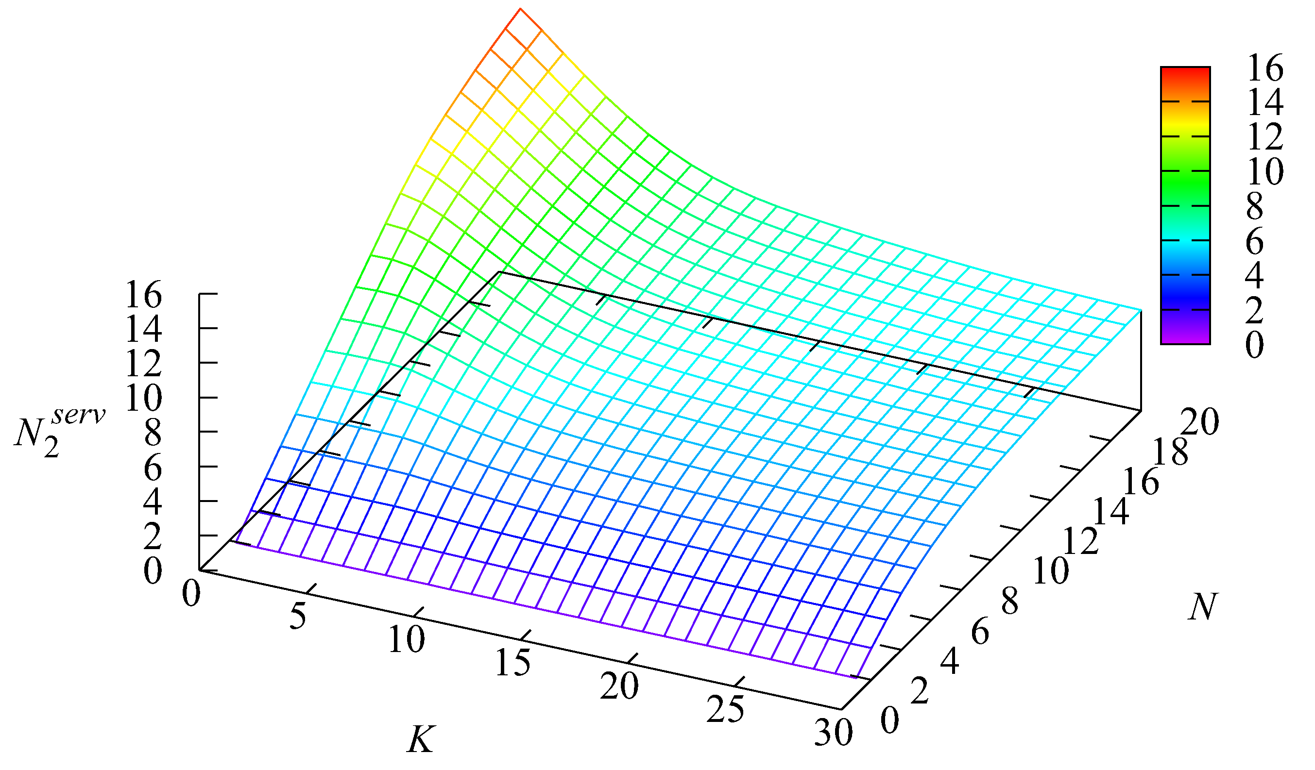
Figure 3 presents the dependence of the average number $N_2^{serv}$ of busy servers in System 2. This number increases when the number N of servers in this system increases. The increase is very essential when K is small and N is large, and thus, many clients jockey to System 2.

Figure 4 presents the dependence of the average number $N_1^{buffer}$ of clients in the buffer of System 1. Generally speaking, this number decreases when K increases and more clients receive service in System 1 without visiting a buffer. However, there are interesting anomalies when the number of servers in System 1 K is small, and it is natural that the queue length in this system is very long. For small $K,$ the initial increase in N leads to a decrease in the number of clients who balk upon arrival. This, in turn, increases the arrival rate of clients in System 1. The further increase in N implies a larger total service rate in System 2 and higher chances that the servers of this system will stay idle and withdraw more clients from the buffer of System 1. Other small irregularities are explained by a complicated form of dependencies of the probabilities $q_{i,n}$ and $p_{i,n}$ on the arguments $(i,n).$

Figure 5 presents the dependence of the average number $N_2^{buffer}$ of clients in the buffer of System 2. The essential decrease in $N_2^{buffer}$ with the increase in K is explained by more intensive jockeying of clients from System 2 because System 1 starts to have more idle servers. A large value of $N_2^{buffer}$ when the number of servers in both systems is small is obvious. The slightly strange behavior of $N_2^{buffer}$ for small N and the initial increase in K is explained by the different forms of the probabilities $q_{i,n}$ and $p_{i,n}$ for $i\le K$ and $i>K.$

Figure 6 presents the dependence of the probability $P_1^{arr}$ that an arbitrary client joins System 1 upon arrival. As it is expected, this probability grows with the increase in the number of servers K because that increase implies that fewer clients wait in System 1. While this leads to a smaller value of balking the system and a larger probability of joining the system. It is natural that the impact of the number K of servers in System 1 is more essential. A small increase in $P_1^{arr}$ for a large number of servers in System 2 is explained by the increase in help for System 1.

Figure 7 presents the dependence of the probability $P_2^{arr}$ that an arbitrary client joins System 2 upon arrival. As expected, this probability is maximal when the number N is large (and System 2 is not overloaded), while System 1 is overloaded due to the small number of existing servers.

Figure 8 presents the dependence of the probability $P_1^{imm}$ that an arbitrary client immediately starts service in System 1. The shape of the surface given in this figure is quite clear because the increase in K implies higher chances that some servers will be idle at an arbitrary client arrival moment. Again, the change in the rate of increase in $P_1^{imm}$ is explained by the piecewise dependence of probabilities $q_{i,n}$ on the arguments $(i,n).$

Figure 9 presents the dependence of the probability $P_2^{imm}$ that an arbitrary client immediately starts service in System 2. This probability is highest when the number N of servers in this system is large compared to the number of servers in the alternative system, which is small.

Figure 10 presents the dependence of the average jockeying intensity $\tilde{\alpha }$ of clients from the buffer of System 1 to the servers of System 2. This intensity is small when the number of servers in System 1 is large enough, and System 1 does need help from servers of System 2. When the number of servers in System 1 is small while the number of servers in System 2 is large, it is natural that the average jockeying intensity $\tilde{\alpha }$ is maximal.

Figure 11 presents the dependence of the average jockeying intensity $\tilde{\gamma }$ of clients from the buffer of System 2 to the servers of System 1. The explanation of the presented surface is exactly the opposite of the explanation of the previous figure.

Figure 12 presents the dependence of the loss probability $P^{loss}$ of an arbitrary client due to the unwillingness to join the system. It is natural that this probability has a maximum when both systems are highly loaded. This occurs when the number of servers in these systems is small. This probability essentially decreases with the increase in at least one or both numbers of servers.

Now, let us demonstrate an opportunity for the application of the obtained results to solving a simple optimization problem. We assume that the quality of the system design is evaluated in terms of the following cost criteria, which have the meaning of the average revenue obtained by the system per unit of time:

$$E=E(N,K)=a({\lambda }_1^{out}+{\lambda }_2^{out})-b\lambda P^{loss}+c\lambda (P_1^{imm}+P_2^{imm})-d_{1}N-d_{2}K$$

where a is the profit earned via providing service to one client, c is the bonus for providing a service to an arbitrary client without waiting in a queue, b is the charge (lost profit) for the balking of one client, $d_1$ is the cost of the use of one server in System 1 per unit of time, and $d_2$ is the cost of the use of one server in System 2 per unit of time.

In this numerical example, we fix the following values of the cost coefficients:

$$a=3,b=3,c=0.02,d_1=0.15,d_2=0.2.$$

We assume that $a=b$ basically because the lost profit may equal the earned profit. However, in general, they can be not equal, e.g., $b>a$ if the balked client not only did not bring a profit right now but may decide to receive service in the future in another competitive service system.

Figure 13 presents the dependence of the cost criterion E on the parameters N and $K.$

It is clear from this figure that the revenue of the system essentially depends on the choice of the numbers K and N of the required servers. The revenue can even turn into a loss if these values are fixed incorrectly, e.g., if the chosen number N of servers in System 2 (number of SSDs) is insufficient.

The optimal value of the cost criterion in this example is $E^{*}=14.0029$ and is reached when $K=17$ and $N=9.$

7. Conclusions

In this paper, we analyzed a queuing system consisting of two multi-server subsystems as a possible model of operation for a supermarket with two groups of counters. In one group, service is provided by human operators. In another group, service is provided by SSDs. An arriving, probably bursty, flow of clients is modeled by the Markovian arrival process. Upon a client’s arrival, he/she observes the lengths of queues in both groups and can decide whether to balk the system or join it. In the latter case, the client additionally decides which system he/she will join. A client that joins some system cannot move to another system unless that system does not have idle servers. The client, which does not see idle servers, can repeat the attempts to jump (jockey) to another system after random time intervals. If the idle servers are available in the target system at the moment of the attempt, the client immediately jockeys to another system and starts service.

The behavior of the considered system is described by a multi-dimensional Markov chain with level-dependent transitions. The generator of this chain is derived, and the stationary distribution of its states is computed. The condition for the existence of this distribution is derived under non-restrictive assumptions about the existence of the limits of probabilities of joining a system and scheduling between the systems when the number of clients in the system infinitely increases. Formulas for the computation of the performance characteristics of the system are presented. Numerical results illustrating the impact of the number of servers on the main performance characteristics of the system are given. The simple optimization problem is solved.

Results can be used for performance evaluation and capacity planning of cooperative systems with different strategies for client admission and scheduling between systems. The possibility of mutual help existing in certain real-world systems in the situation where one of the systems has idle servers is taken into account. Results can be used for the optimization of a variety of real-world systems where human servers can be used along with the SSDs and other systems with possible joint use of the available resource (e.g., channel bandwidth) by several service providers. Future research should consider rating-dependent arrival (see, for example, [22]) of inhomogeneous clients based on their initial preference of the system to service, as well as the phase-type distribution of service time in System 1.